In this paper, we describe our implementation of a primal-dual infeasible-interior-point algorithm for large-scale linear programming under the MATLAB1 ...
Solving Large-Scale Linear Programs by Interior-Point Methods Under the MATLAB Environment � Yin Zhang Department of Mathematics and Statistics University of Maryland Baltimore County Baltimore, Maryland 21228-5398
Technical Report TR96-01 February, 1996
Abstract In this paper, we describe our implementation of a primal-dual infeasible-interior-point algorithm for large-scale linear programming under the MATLAB1 environment. The resulting software is called LIPSOL { Linear-programming Interior-Point SOLvers. LIPSOL is designed to take the advantages of MATLAB's sparse-matrix functions and external interface facilities, and of existing Fortran sparse Cholesky codes. Under the MATLAB environment, LIPSOL inherits a high degree of simplicity and versatility in comparison to its counterparts in Fortran or C language. More importantly, our extensive computational results demonstrate that LIPSOL also attains an impressive performance comparable with that of e�cient Fortran or C codes in solving large-scale problems. In addition, we discuss in detail a technique for overcoming numerical instability in Cholesky factorization at the end-stage of iterations in interior-point algorithms.
Keywords: Linear programming, Primal-Dual infeasible-interior-point algorithms,
MATLAB, LIPSOL.
Abbreviated Title: Solving Large Linear Programs under MATLAB
� 1
This work was supported in part by DOE DE-FG02-93ER25171-A001. MATLAB is a registered trademark of The MathWorks, Inc.
1
1 Introduction After over a decade of extraordinarily active research triggered by the seminal work of Karmarkar [5], the eld of interior-point methods has nally come to maturity as far as linear programming is concerned. Not only do we have a solid theoretical foundation for interior-point methods for linear programming, but also a rather comprehensive understanding on their practical e�ciency. Among many general algorithmic approaches, the most e�ective one in practice has proven to be the primal-dual infeasible-interior-point approach, including a number of variants and enhancements such as Mehrotra's predictor-corrector technique [13]. Recent experiments indicate that as the problem size increases, so does the frequency of interior-point methods outperforming the classic simplex method [12]. This trend has been observed for a while but is becoming more pronounced recently. In our opinion, this marks the beginning of a new era in which interior-point methods coexist with the simplex method but gradually assume the role of dominant computational engine for general large-scale linear programming Beside computational e�ciency, another advantage of interior-point algorithms is that their implementations for large-scale linear programming, through still quite involved, are considerably simpler than those for the simplex algorithms. This is particularly true under a high-level programming environment such as MATLAB that supports high-level sparse-matrix operations. The main purpose of the paper is to describe our implementation of a large-scale primal-dual infeasible-interior-point algorithm under the MATLAB environment and to present computational results. Hence we will concentrate on the implementation aspects of interior-point methods. There is a vast volume of literature on the theoretic aspects of interior-point methods. We refer interested readers to the Interior Methods Online web page at the Argonne National Laboratory 2 for more informations on interior-point methods, including a comprehensive bibliography containing works up to 1993. For survey papers concerning computation and implementation issues, we refer readers to [11] and [1]. In Section 2, we describe the general framework for primal-dual infeasible-interior-point algorithms. We present the framework as a modi ed form of the well-known Newton's method and give intuitions to justify the modi cations to the Newton method. These motivations are easily understandable to readers with a basic knowledge on Newton's method. In doing so, we hope that this section can also serve a pedagogical purpose. Readers who are familiar with interior-point algorithms may choose to skip parts of Section 2. Section 3 is a brief description of the MATLAB technical computing environment under which 2
URL: http://www.mcs.anl.gov/home/otc/InteriorPoint/index.html
2
we developed our software LIPSOL. We discuss a number of major issues in implementation in Section 4. Section 5 is devoted to discussing a technique for overcoming numerical instability in Cholesky factorization. Numerical results are presented in Section 6 and nally concluding remarks in Section 7.
2 Infeasible-Interior-Point Methods In this section, we will motivate the formulation of primal-dual infeasible-interior-point methods from a practical algorithmic point of view, exploring the close tie between the classic Newton's method and the primal-dual infeasible-interior-point methods. We start from a description of linear programming.
2.1 Linear Programming We consider the following primal linear program: (1)
min s.t.
cT x Ax = b 0 � x i � ui i 2 I 0 � xi i2J
where A 2 Rm�n , which determines the sizes of other vectors involved, and I and J are disjoint index sets such that I [ J = f1; 2; � � � ; ng and I \ J = ;. Without loss of generality, let us assume that for some positive integer nu � n (2)
I = f1; 2; � � � ; nug; and J = fnu + 1; nu + 2; � � � ; ng:
Given a vector x in Rn , we use the notation xu for the vector in Rnu whose elements are the rst nu elements of x, i.e., [xu ]i = xi ; i = 1; 2; � � � ; nu : Moreover, we de ne the appending operator \app" from Rnu to Rn that appends n ? nu zeros to vectors in Rnu , i.e., for w 2 Rnu
8 < w ; 1 � i � nu (3) [app(w)]i = : i 0; nu < i � n: By adding the slack variables s 2 Rnu , we can rewrite the above linear program into the standard 3
form:
min s.t.
(4)
cT x Ax = b xu + s = u x � 0; s � 0
The dual of the above standard primal linear program is: max bT y ? u T w (5) s.t. AT y + z ? app(w) = c z � 0; w � 0 where y, z and w are the dual variables and slacks. It is well-known that the solutions of the primal and the dual linear programs, if they exist, satisfy the following KKT conditions which is a system of linear-quadratic equations with nonnegativity constraints on some variables:
1 0 Ax ? b CC BB xu + s ? u CC BB T B F (x; z; s; w; y) = BA y + z ? app(w) ? cC CC = 0; (x; z; s; w) � 0; BB CA xz @
(6)
sw
where xz and sw denote component-wise multiplications and the equations xz = 0 and sw = 0 are called the complementarity conditions for the linear program. For nonnegative variables x; s; z; w, we will call the quantity xT z + sT w the duality gap (regardless of feasibility or infeasibility of these variables). The duality gap measures the residual of the complementarity portion of F in `1 -norm when (x; z; s; w) � 0. A straightforward calculation shows that the Jacobian matrix of F (x; z; s; w; y) is 3 2 A 0 0 0 0 7 66 T 66 E 0 Iu 0 0 777 (7) F 0 (x; z; s; w; y) = 66 0 I 0 ?E AT 77 : 7 66 4 Z X 0 0 0 75 0 0 W S 0
h
i
where E T = Iu 0 , Iu is the identity matrix of dimension nu , X = diag(x), Z = diag(z ), S = diag(s) and W = diag(w). Unlike a primal (dual) method which concentrates on solving the primal (dual) program, a primal-dual interior-point method for linear programming solves the KKT system (6), which includes all the primal and dual variables and slacks. 4
2.2 Newton's Method and Variants It is clear from (6) that solving a linear program is equivalent to solving a system of linearquadratic equations with nonnegativity constraints on a subset of variables. In order to simplify our coming discussion, we rewrite the KKT system (6) into a constrained algebraic system of ` equations and ` variables with nonnegativity constraints on `+ variables:
F (v) = 0; vi � 0; 1 � i � `+;
(8)
where v = (x; z; s; w; y), ` = 2n + 2nu + m and `+ = 2n + 2nu. Let us rst drop the nonnegativity constraints from (8) and consider Newton's method for solving an unconstrained system of nonlinear equations
F (v) = 0; which can be written as (9)
vk+1 = vk ? F 0 (vk )?1 F (vk ):
It is well-known that Newton's method has excellent local convergence properties. More speci cally, if the Jacobian matrix F 0 (v) is nonsingular and Lipcshitz continuous at a solution v� , and the initial point v0 is su�ciently close to v� , then the iterate sequence fvk g converges to v� Q-quadratically. On the other hand, Newton's method generally does not have very good global convergence properties. A variant of Newton's method is called the damped Newton: (10)
vk+1 = vk ? �k F 0 (vk )?1 F (vk );
which introduces a damping factor, or step length, �k , usually chosen from the interval (0; 1], to enhance global convergence. Another variation of Newton's method is the so-called composite Newton's method. At each iteration, it calculates an intermediate point v^k and uses the same Jacobian matrix twice:
v^k = vk ? F 0 (vk )?1 F (vk ); vk+1 = v^k ? F 0(vk )?1 F (^vk ): Equivalently, we can shorten the expression as (11)
vk+1 = vk ? F 0 (vk )?1 (F (vk ) + F (^vk )):
In terms of linear algebra work, the composite Newton requires one matrix factorization per iteration, same as for Newton's method, but two back-solves instead of one. Since matrix factorizations are usually much more expensive than back-solves (O(n3 ) vs. O(n2 ) for dense matrices), 5
the required work per iteration for the composite Newton is comparable with that for Newton's method. However, under similar conditions, the composite Newton has a Q-cubic asymptotic convergence rate, one order faster than that of Newton's method. Similarly, one can introduce a damping factor into the composite Newton's method: (12)
vk+1 = vk ? �k F 0 (vk )?1 (F (vk ) + F (^vk )):
For more detailed information on Newton's method and its variants, we refer to the classic book by Ortega and Rheinboldt [16].
2.3 Infeasible-Interior-Point Methods Let us now go back to the nonnegativity constrained system of equations (8) that represents a linear programming in a simpli ed notation. We recall that for linear programming, F (v) contains only linear and quadratic equations and the quadratic ones are complementarity pairs. Obviously, in the presence of the nonnegativity constraints for the rst `+ variables we cannot expect to obtain a nonnegative solution by just simply applying the Newton's method. However, a crucial observation is that the damped Newton (10) will generate a sequence of iterates fvk g that satis es the nonnegativity constraints if (i) we start from a initial point v0 whose rst `+ components are positive, i.e., vi0 > 0; 1 � i � `+ , and (ii) we choose the step-length � at each iteration so that these rst `+ components remain positive in all the subsequent iterations. It is important to note the necessity of keeping the nonnegative variables (the rst `+ component) strictly positive at every iteration instead of just nonnegative. Consider a complementarity condition sw = 0. The Newton equation (i.e., the linearized equation) for sw = 0 at a given point (s; w) is s�w + w�s = ?sw. If one variable, say wi , is zero, then the Newton equation becomes si �wi = 0, leading to a zero update �wi = 0. Consequently, wi will remain zero all the time once it becomes zero. This is fatal because an algorithm will never be able to recover once it sets a variable to zero by mistake. Therefore, it is critical to keep the nonnegative variables strictly positive at every iteration, not just nonnegative. Even keeping nonnegative variables strictly positive, one would still expect di�culty in recovering from a situation where a variable is adversely set to too small a value. To decrease the chances of such mistakes at early stages, it would be desirable that all the complementarity pairs converge to zero at the same pace, say ski wik = �k ! 0 as k ! 1 for every index i. Towards this goal (and for other theoretic considerations as well), one can perturb each complementarity condition si wi = 0 into si wi ? � = 0 and let � go to zero in a controlled fashion. This idea, incorporated into the damped Newton (10), leads to the following framework: choose v0 such that 6
all the linear equations in F (v) = 0 (i.e., feasibility equations) are satis ed and vi0 > 0; i � `+ ; for k = 0; 1; � � � , do vk+1 = vk ? �k F 0 (vk )?1 (F (vk ) ? �k e^); where �k > 0, �k > 0 is chosen such that vik+1 > 0; i � `+ , and the vector e^ 2 Rn is de ned as
8 > :1; if Fi(v) is quadratic.
Clearly, this de nition indicates that perturbations are only applied to the complementarity conditions, which are all quadratic, but not to the feasibility conditions, which are all linear. The above primal-dual interior-point approach was rst proposed by Kojima, Mizuno and Yorshisi [6], in which a feasible initial point is required and the linear equations are always satis ed. According to the classi cation introduced in [19], this type of methods is called feasibleinterior-point methods. Lustig, Marsten and Shanno [9] implemented a modi ed version of the Kojima-MizunoYorshisi interior-point approach. A fundamental modi cation is the removal of the requirement for a feasible initial point which is practically undesirable. The Lustig-Marsten-Shanno algorithm can be schematically cast into the following infeasible-interior-point (IIP) algorithmic framework:
Algorithm IIP-1:
Choose an initial point v0 such that vi0 > 0; 1 � i � `+ . Set k = 0. Do until kF (vk )k is \small" (1) Choose �k > 0 and compute �vk = ?F 0 (vk )?1 (F (vk ) ? �k e^). (2) Choose �k > 0 and set vk+1 = vk + �k �vk such that vik+1 > 0; 1 � i � `+ . Increment k by 1.
End
Mehrotra [13] introduced an enhanced version of the infeasible-interior-point algorithm that he called a predictor-corrector method. It was observed in [17] that Mehrotra's algorithm can also be considered as a modi cation to the damped composite Newton's method (12), which is schematically very close to the following algorithmic framework:
7
Algorithm IIP-2:
Choose an initial point v0 such that vi0 > 0; 1 � i � `+ . Set k = 0. Do until kF (vk )k is \small" (1) Compute �p vk = ?F 0 (vk )?1 F (vk ) and determine �k > 0. (2) Compute �c vk = ?F 0 (vk )?1 (F (vk + �p vk ) ? �k e^). (3) Choose �k > 0 and set vk+1 = vk + �k (�p vk + �c vk ) such that vik+1 > 0; 1 � i � `+ . Increment k by 1.
End
In this framework, two steps are computed at each iteration: the predictor step �pvk and the corrector step �cvk , both using the same matrix factorization. Extensive computational experiments [10, 13] have indicated that Mohrotra's infeasible-interior-point framework is by far the most e�cient interior-point framework in practice. It usually requires considerably less iterations than algorithms in the framework of Algorithm IIP-1. Furthermore, since it requires only one matrix factorization per iteration, it is more e�cient than algorithms based on the Mizuno-Todd-Ye [14] predictor-corrector approach which requires two matrix factorizations per iteration. For proper choices of parameters and starting points, the global convergence and computational complexity of Algorithm IIP-1 were rst established in [7] and [19], respectively; and the computational complexity of Algorithm IIP-2 was rst established in [21]. There are a number of e�ective enhancements to Algorithm IIP-2. Xu et al [18] proposed and implemented a homogeneous and self-dual algorithm which applies the basic framework of Algorithm IIP-2 to a homogeneous and self-dual reformulation of a linear program. At the cost of some extra work at each iteration, this algorithm can more reliably detect infeasibility. Hence in the case of solving untested models with unknown feasibility, the homogeneous and selfdual algorithm may be preferable. Recently, Gondzio [4] proposed a technique called multiple centrality corrections that can further reduce the number of iterations required for convergence by adaptively adding one or more corrector steps to the framework of Algorithm IIP-2.
3 The MATLAB Environment Our implementation was done under the MATLAB environment. MATLAB, standing for matrix laboratory, is a high-level technical computing environment for numeric computation and visualization. It integrates numerical analysis, matrix computation and graphics in an easy-touse environment where matrix-computational formulas can be expressed in MATLAB scripts, 8
called M- les, that are very close to what they would be written mathematically - thus avoiding low-level programming as is needed in Fortran or C programming. Because of this advantage, development-time in MATLAB is much shorter than in other languages such as Fortran and C. However, for computation-intensive tasks overhead incurred in MATLAB generally makes it slower, which is a price one has to pay in exchange for programming simplicity. MATLAB provides external interface facilities to enable interaction with programs written in Fortran or C languages in the form of the MEX- les, where MEX stands for MATLAB Executable. MEX- les are dynamically linked subprograms compiled from C or Fortran source code that can be called and run from within MATLAB in the same way as MATLAB M- les or built-in functions. The external interface functions provide functionality to transfer data between MEX- les and MATLAB. Our implementation includes both M- les and MEX- les. The routine tasks, mostly matrix and vector operations, are done by M- les, while the most computation-intensive tasks are done by MEX- les generated from Fortran programs. This combination enables us to take advantage of both worlds: programming simplicity in MATLAB and computational speed in Fortran.
4 Implementation Details Our implementation is based on the framework of Algorithm IIP-2. We still need to specify the following: (1) the initial point and the stopping criteria; (2) how to compute the steps; and (3) how to choose the parameters �k and �k . As in most implementations, we use di�erent step lengths in the primal and dual spaces to achieve better e�ciency. In addition, there are a number of implementation issues that usually do not appear in algorithms but are extremely important to the quality of software. These include the exploitation of sparsity and the treatment of numerical instability as well as dense-columns. We will discuss these issues in some detail. The software package resulted from our implementation, currently for UNIX systems only, is called LIPSOL (Linear-programming Interior Point SOLvers). LIPSOL runs under MATLAB version 4.0 and above.
4.1 Preprocessing, Starting and Stopping The purpose of preprocessing is to transform a given linear program into the standard form (see (1)) and get rid of some redundancy from the formulation. Currently, the de facto industrial standard input format for linear programs is the MPS format (see [15] for an introduction to the MPS format). LIPSOL includes an MPS reader program mps2mat to read MPS les and 9
translate the data into MATLAB data les. In the MPS reader, a free variable is split into the di�erence of two nonnegative variables. The preprocessing function preprocessing.m performs a number of tasks such as checking obvious infeasibility, deleting xed variables and zero rows and columns from the matrix A, solving equations with only one variables and shifting nonzero lower bounds to zero, whenever any of these events occurs. The scaling function scaling.m performs a row and a column scaling to the matrix A. We believe that those scalings help the solution process in some way, though we do not have hard evidence on how much bene ts these scalings actually bring. The M- le initpoint.m chooses starting point for iterations. The starting-point selection in LIPSOL basically follows the one used in [10] with some minor modi cations. The function stopping.m tests stopping criteria and, if any met, terminates the iterations. The main stopping criterion is the standard one: krb k + krc k + kRuk + jcT x ? bT y + uT wj � tol (13) max(1; kbk) max(1; kck) max(1; kuk) max(1; jcT xj; jbT y ? uT wj) where rb = Ax ? b, rc = AT y + z ? app(w) ? c and ru = xu + s ? u are, respectively, the residuals in primal, dual and upper-bound feasibility, cT x ? bT y + uT w is the di�erence between the primal and dual objective values, and tol is the tolerance which is set to 10?8 by default. The sum on the left measures the total relative errors in the KKT system (6). A number of heuristics are also included to detect infeasibility, though they have not been well tested on infeasible problems at this point and may change over time.
4.2 Centering and Step-Length Parameters The centering parameter �k is computed by the function centering.m. It is chosen largely as suggested by Mehrotra [13] but with some minor modi cations. The value of �k is a fraction of the normalized duality gap T T g(x; z; s; w) = x nz ++ns w u k k k k evaluated at the current iterate (x ; z ; s ; w ), i.e.,
�k = �k gk ; for some �k 2 (0; 1). After computing the predictor step �p vk . A ratio test is performed to determine �^ p such that (^x; s^) = (xk ; sk ) + min(1; �^p )(�p xk ; �p sk ) 10
is either positive in the case �^ p > 1 or on the boundary of the nonnegative orthant (x; s) � 0 in the case �^ p � 1. Similarly, we compute (^z ; w^ ) = (z k ; wk ) + min(1; �^d )(�pz k ; �p sk ) such that it is either positive or on the boundary of the nonnegative orthant (z; w) � 0. The parameter �k is then set to !2 T z^ + s^T w^ x ^ k � = (xk )T zk + (sk )T wk : The above choice was rst suggested by Mehrotra [13]. We also impose an upper bound on �k at each iteration to limit �k to a value smaller than one. At the early stage of the iterations, we set the upper bound to a value around 0:2. Near the end we force it to be in the same order as the total relative error. This strategy is designed to achieve fact local convergence at the end stage of the iterations. Let us recall the notation v = (x; z; s; w; y) and de ne (�xk ; �z k ; �sk ; �wk ; �yk ) � �vk = �p vk + �c vk ; i.e., the combined predictor-corrector step. The primal and dual step-length parameters �kp and �kd at each iteration are chosen so that the new iterate
1 0 k+1 1 0 k 1 0 � �xk x x p C BB k+1 CC BB k CC BB BB z CC BB z CC BB �d �zk CCC vk+1 � B BB sk+1 CCC = BBB sk CCC + BBB �p �sk CCC B@wk+1CA B@wk CA B@�d �wk CA yk+1
yk
�d �yk
lies on or just inside the boundary of the set
N = fv : (x; z; s; w) > 0; min(xz; sw) � �0 g(x; z; s; w)g; where �0 = 10?5 by default. It is known that the membership in N guarantees the positivity of (x; z; s; w). The set N is often referred as a neighborhood of the (generalized) central path de ned as the set
C = fv : (x; z; s; w) � 0; min(xz; sw) = max(xz; sw)g; i.e., the components of the vectors xz and sw are all the same and, of course, equal to their average g(x; z; s; w). Staying in N prevents the elements of (x; z; s; w) from becoming too close to zero at an early stage. 11
In our implementation, we use a back-tracking strategy to ensure that the new iterate vk+1 is on the boundary or just inside of N . We start with (�p ; �d ) = �0 (��p ; �� d ) where (��p ; �� d ) are computed by ratio tests and �0 is set to 0:9995 by default, and repeatedly decrease (�p ; �d ) by a certain factor, if needed at all, until the de ning inequality of the set N is satis ed. This process is implemented in the function update.m.
4.3 Computing the Steps The major computation at each iteration is to solve the a system with the coe�cient matrix F 0(v) (see (7)) and two di�erent right-hand sides, one for the predictor direction and the other for the corrector one. Both right-hand sides can be written in terms of vectors rb ; ru ; rc ; rxz and rsw . More speci cally, the right-hand sides for the predictor and the corrector directions are, respectively, the negative of the following two vectors: 1 0 1 0 1 0 1 0 r 0 r Ax ? b b b CC BB CC BB CC B C BB B ru C B 0 ru C xu + s ? u CC B C B B C CC and BB CC = BB B CC = BB T CC B 0 rc C BA y + z ? app(w) ? cC BB rc CC BB B C B B C B@ rxz CA B@ (�pxk )(�pzk ) ? �k en CCA CA B xz @rxz CA B@ (�p sk )(�p wk ) ? �k enu rsw sw rsw where en and enu are vector of all ones of dimension n and nu, respectively. It is worth noting that the rst vector is just F (vk ), and the second F (vk + �pvk ) subtract the perturbation vector involving �k . Since F 0 (v) is a highly structured sparse matrix, one can solve it by block Gaussian elimination which leads to the following procedure for both the predictor and the corrector steps corresponding to di�erent right-hand sides:
Procedure Steps:
(1) Form the matrix D = [X ?1 Z + diag(app(S ?1 w))]?1 . (2) Overwrite: rc ( rc ? X ?1 rxz + app(S ?1 (rsw ? Wru). (3) Solve for �y by Cholesky factorization from the linear system: (ADAT )�y = ?(rb + ADrc). (4) Compute �x = DAT (�y + rc ), �z = ?X ?1 (Z �x + rxz ), �s = ?(�xu + ru ), �w = ?S ?1 (W �s + rsw ). 12
This procedure is implemented in the M- le direction.m. Similar procedures were used in earlier implementations, see [9], [10] and [13].
4.4 Sparse Cholesky Factorization For our large-scale interior-point code, the major computation at each iteration is in step (3) of Procedure Steps where the coe�cient matrix ADAT is formed and factored. Since D is a positive diagonal matrix, if A has full rank ADAT is positive de nite with the same sparsity pattern as AAT . The e�ciency of a large-scale interior-point code lies predominantly on the e�ciency of the sparse Cholesky factorization code used. Cholesky factorization of a sparse matrix, say P = LLT where L is lower triangular, generally involves three stages. First one need to reorder the rows and columns of the matrix P in an attempt to minimize the llings { the new nonzero elements created during factorization. Then one performs a symbolic factorization to gure out the sparsity pattern of L. Finally, one carries out the actual factorization. In the context of interior-point algorithms, since the sparsity pattern of P = ADAT , disregarding cancelation, remains the same for any positive diagonal matrix D, one only need to perform an ordering and a symbolic factorization once at the very beginning. MATLAB does provide functions for ordering and factoring a sparse symmetric positive de nite matrices. However, for the sake of numerical stability, we must be able to modify the standard Cholesky factorization procedure (see Section 5). This can not be done under MATLAB since source code access is unavailable for MATLAB's build-in functions. Therefore, we decided to use MATLAB's external interface facilities and existing Fortran sparse Cholesky code in our LIPSOL implementation. We constructed MEX- les from two Fortran packages: a sparse Cholesky factorization package (version 0.3) developed by Esmond Ng and Barry Peyton at the Oak Ridge National Laboratory (ORNL), and a multiple minimum-degree ordering package by Joseph Liu at University of Waterloo which is included in the ORNL package. The ORNL package uses relatively new techniques such as supernode block factorization to take advantage of modern computer architectures [8].
4.5 Dense Columns Let us denote the i-th column of A by ai . It is clear from
ADAT
=
m X i=1
dii ai aTi
that ADAT will be generally dense as long as there is one dense column in A. Although for most large-scale applications the occurrence of dense columns is rare, it does occur from time to time 13
and must be dealt with. Our strategy for dense columns, like in many other codes, is to split the relatively dense columns, if any, from the sparse ones to form
ADAT = P + UU T where P is the product of the sparse columns and U is the collection of dense columns multiplied by corresponding diagonal elements of D1=2 . Matrix U usually has a very low rank. If P is nonsingular, then by the Sherman-Morrison formula (P + UU T )?1 = P ?1 ? P ?1 U (I + U T P ?1 U )?1 U T P ?1 ; the solution to the linear system (P + UU T )�y = h is �y = h^ ? P ?1 U (I + U T P ?1 U )?1 U T h^ ; where h^ = P ?1 h. Of course, we never compute any inverse matrices, but just solve the relevant linear systems. Since U has very low rank, the matrix I + U T P ?1 U is very small and requires a small number of back-solves to form once P is factored. This approach is not always stable because P , the sparse portion of ADAT , can be severely ill-conditioned or actually singular. To stabilize the process, we utilize a preconditioned conjugate gradient method whenever we nd the residual for the solution from the Sherman-Morrison formula is unsatisfactory. The pre-conditioner is constructed from the Cholesky factor of P = LLT (possibly modi ed, see Section 5). Recall that the system we want to solve is (LLT + UU T )�y = h: Our preconditioned conjugate gradient method mathematically amounts to applying the conjugate gradient method to the following preconditioned, equivalent system [I + (L?1 U )(L?1 U )T ]��y = h� ; where ��y = LT �y and h� = L?1 h. The new coe�cient matrix generally has a better eigenvalue distribution. This combination of the Sherman-Morrison formula and preconditioned conjugate gradient method was proposed in Choi, Monma and Shanno [2]. Throughout the computation, we only factor the sparse portion of the matrix ADAT . Computational results have shown that the above dense column strategy performs adequately for the Netlib set of test problems (see Section 6 for a description of the Netlib set). The implementations of the Sherman-Morrison formula and the preconditioned conjugate gradient method are, respectively, sherman.m and pcg.m. 14
5 Numerical Stability in Cholesky Factorization It is well known that in a primal-dual interior-point method the Jacobian matrices at any primal degenerate solution is necessarily singular. In Procedure Steps, this singularity is re ected in the matrix P = ADAT where D is a diagonal matrix varying from iteration to iteration. It is known that for linear programming all solutions in the relative interior of a non-singleton solution set satisfy the strict complementarity (14)
xz = 0; x + z > 0; sw = 0; s + w > 0:
This implies that the diagonal elements of D either approach zero or in nity, as can be seen from the construction of D. Whenever D has too many small diagonal elements, near-singularity could occur and the standard Cholesky factorization may become unstable in that very small diagonal pivots are encountered. For degenerate problems, this near-singularity can cause illconditioning so severe that it often prevents the standard Cholesky factorization method from getting an acceptable approximate solution. In this section, we discuss in detail a technique for overcoming the numerical instability encountered in Cholesky factorization. Similar techniques have been used in earlier implementations such as in OB1 [9]. However, we have not seen any discussion in the literature on the theoretical foundation and justi cation for these techniques. In the sequel, we will motivate and construct a mathematically well-founded procedure for treating numerical instability in Cholesky factorization in the context of interior-point algorithms. Let us de ne for a strict complementary solution v� = (x� ; z � ; s� ; w� ; y� ) the index sets (15) (16)
B = fi : x�i > 0 and x�i < ui for i � nug; N = fi : x�i = 0 or x�i = ui for i � nug:
It is well-known that these index sets are invariant with respect to the choices of strict complementary solution v� . Without loss of generality, let us assume that for some positive integer
p�n
(17)
B = f1; 2; � � � ; pg; N = fp + 1; p + 2; � � � ; ng:
Now consider the linear system in step (3) of the Procedure Steps (18)
ADAT �y = ?(rb + ADrc);
where rb = Ax ? b. As the iterates approach the interior of the solution set, from the de nition 15
of D we see that
8 > :0; i 2 N :
(19)
We introduce the following partitioning in terms of the index sets B and N speci ed in (15), (16) and (17) for the matrices D, A and rc:
3 0 1 2 D 0 B 5 ; A = [AB AN ]; rc = @(rc)B A : D=4 0
DN
(rc )N
Using this partitioning, we rewrite the linear system (18) as (20)
(AB DB ATB + AN DN ATN )�y = ?(rb + AB DB (rc )B + AN DN (rc)N ):
As the iterates converge to the solution set, we know that DB ! 1, DN ! 0 and rb ! 0. Moreover, the overwritten rc (see (2) in Procedure Steps) is bounded under normal conditions. Hence we have the following asymptotic behavior for terms in (20):
AB DB ATB ! 1; AN DN ATN ! 0; AB DB (rc)B ! 1; AN DN (rc )N ! 0: As a result, in a small neighborhood of the solution set linear systems of the form (20) are all small perturbations to the the following consistent linear system (21)
(AB DB ATB )�y = ?AB DB (rc )B :
If the rank of AB is less than m, such as in the case of degeneracy where p < m, then AB DB ATB is singular. Consequently, as the iterates progresses towards the solution set, we encounter increasingly ill-conditioned or even numerically singular systems. In this case, the standard solution procedure based on Cholesky factorization will break down and fail to return an acceptable approximate solution. Unfortunately, in practical applications degeneracy occurs surprisingly often. Therefore, in order to have a robust and accurate interior-point code one must be able to solve to an acceptable accuracy the linear system (21) as well as arbitrarily small perturbations to it. Let us now consider solving (21). Without loss of generality, we assume that (i) AB has full rank p but p < m, and (ii) the rst p rows of AB is linearly independent. The second assumption implies that the rst p rows, and columns by symmetry, of AB DB ATB are linearly independent. 16
However, we would like to avoid to be directly involved in the partitioning of B and N and prefer to have a single algorithm that can stably solve (18) in all situations, be it far away from or close to the solution set. So later when we construct the algorithm, we will assume no knowledge on the speci c structure of the coe�cient matrix P except that it is symmetric positive semide nite but not necessarily de nite. Now suppose that we are given the coe�cient matrix P and right-hand side h, where
P = AB DB ATB ; h = ?AB DB (rc)B ; and want to solve
P �y = h:
(22)
This linear system has multiple solutions. Fortunately, it is known that the convergence theory for primal-dual interior-point algorithms only require a solution to (18), so any solution will su�ce. We make a further partitioning by grouping the rst p rows and the last (m ? p) rows of A, y and h: 0 1 0 1 2 13 � y A 1 AB = 4 B2 5 ; �y = @ A ; h = @h1 A : h2 �y2 AB By our assumption, A1B is a p � p nonsingular matrix. From the transpose of QR decomposition, there exists a p � p orthogonal matrix Q such that
AB
2 3
L D1=2 = 4 5 Q B
M
where L is p � p, lower triangular and nonsingular. It is not di�cult to see that (23)
32 T T3 2 2 3 i h L 05 4L M 5 L P = AB DB ATB = 4 5 LT M T = 4 M 0
M
0
0
and the right-hand side is nothing but the Cholesky factorization of P . Moreover, all the solutions of (22) are given by the rst p linearly independent equations (LLT )�y1 + (LM T )�y2 = h1 : In particular, we are interested in the so-called basic solution (24)
0 ?T ?1 1 L L h1 A �y� = @ ; 0
corresponding to �y2 = 0. 17
For convenience of discussion, in the sequel we will use the extended arithmetic; namely, we will include 1 (only positive in nity will su�ce for our purpose) as a real number such that 1=1 = 0. Let us de ne D1 as the (m ? p) � (m ? p) diagonal matrix with in nity on the diagonal ?1 = 0. and as a result D1 Replacing the zero diagonal blocks by D1 in the Cholesky factors of P in (23), we obtain the following matrix product associated with P ,
2 L P )4
32
3
0 5 4LT M T 5 : M D1 0 D1
(25)
We will call (25) the Cholesky-In nity factorization of the positive semide nite matrix P . We now show that the basic solution �y� given in (24) is the uniquely solution to the extended system associated with the Cholesky-In nity factorization of P :
2 4L
32
30
1 0 1
0 5 4LT M T 5 @�y1 A @h1 A = : M D1 0 D1 �y2 h2
(26)
This system can be solved by the forward and backward substitution procedure
2 4L
30 1 0 1
2
30
1 0 1
0 5 @t1 A @h1 A LT M T 5 @�y1 A = @t1A ; = and 4 M D1 t2 h2 0 D1 �y2 t2
which leads to
t1 = L?1 h1 ; ?1 (h2 ? Mt1 ) = 0; t2 = D1 ?1 t2 = 0; �y2 = D1 �y1 = L?T (t1 ? M T �y2 ) = L?T L?1 h1 ; namely, �y = �y� . Therefore, solving (22) for the basic solution reduces to nding the CholeskyIn nity factorization of P . We provide a simple modi cation to the Cholesky factorization procedure to obtain an algorithm that will return the Cholesky factorization for a positive de nite matrix, but the Cholesky-In nity factorization for a positive semide nite, but not de nite, matrix. A (column version) Cholesky factorization procedure for P = LLT , where P = [pij ] is symmetric and L = [`ij ] is lower triangular, can be written as follows.
18
Procedure Cholesky: For j = 1 : n 2 d = pjj ? Pkj?1 =1 `jk (diagonal pivot). If d 0 and huge dhuge > 0: If d = 0, then set d = 1. =) If d < dtiny , then set d = dhuge. This modi cation enables the procedure to solve not only (21) but also its small perturbations in a stable manner. Extensive computational experiments have proved that the above strategy works surprisingly well in general. In practice, it e�ectively circumvents numerical di�culty encountered in the standard Cholesky factorization procedure and can attain an accuracy up to the square root of the machine epsilon and beyond.
6 Numerical Results In this section, we describe our numerical experiments and present computational results. Our numerical experiments were performed on a Silicon Graphics Challenge XL computer at the University of Maryland Baltimore County. It is a shared-memory, symmetric multi-processor machine with 20 MIPS R4400/150MHz CPU's, 1 gigabytes of memory, and 16k data cache per processor (plus 16k instruction cache and 1 Mbyte secondary cache). Since we always used only a single processor at a time, our numerical results can be reproduced on a single processor workstation with the same CPU and ample memory (say, 128 Mbytes). The test problems used in our experiments were the Netlib set of linear programs. Netlib set is an electronically distributed collection of linear programs originated and maintained by David Gay [3] at the Bell Laboratory. As of January of 1996, the collection consists of 95 problems, including a number of fairly large problems from real-world applications. The sizes of the problems range from a few dozen variables to over fteen thousands. Over the years, the Netlib set has become the standard set of test problems for testing and comparing algorithms and software for linear programming.
6.1 Test Results for LIPSOL We tested LIPSOL v0.3 on all the 95 linear programming problems in the Netlib test set. We tabulate the test results in Tables 2-4 in the Appendix. In each table, the seven columns give, respectively, the problem name, the number of constraints in the unprocessed model, the number of variables in the unprocessed model, the number of iterations required for convergence, the total relative residual as given by (13), the primal objective value and the CPU seconds.
20
6.2 Fortran Package OB1 OB1 (Optimization with Barrier 1) was developed by Irv Lustig, Roy Marsten and David Shanno. Their work [9], largely based on the OB1 package, won the Orchard-Hays Prize from the Mathematical Programming Society in 1991 as the best computational research of the year. Until its retirement in 1993, OB1 was widely recognized as the best interior-point code for linear programming. The version of OB1 available to us and used in our experiments was version 5.0 released in 1991. We understand that the nal version of OB1 was version 6.0, which contained enhancements and improvements to version 5.0. Our purpose is to compare qualitatively the performance of LIPSOL v0.3 with an e�cient interior-point code written in Fortran or C. In addition to its availability to us, OB1 version 5.0 is well suited for this purpose of comparison since, being the best interior-point code during the 1991-1992 period, it is still an adequately e�cient code even by today's standard. We compiled OB1 version 5.0 under SGI IRIX 5.3 F77 compiler using the ags -O -mips2. These same ags were also used to compile the MEX- les in LIPSOL. We used all the default options to run OB1 version 5.0 except specifying the cache size as 16k.
6.3 Comparison with OB1 We also solved all 95 Netlib problems using OB1 version 5.0 on the same SGI computer. Since the purpose of the comparison was to qualitative rather than quantitative to save space we will not list all the computational results obtained for OB1. Instead, we will summarize the comparison by a graph in Figure 1. Our general observation is that for most problems, in particular for the smaller problems, LIPSOL v0.3 is slower than OB1 5.0, but for the a few largest problems LIPSOL v0.3 performs as well as, or even slightly better than, OB1 5.0. To capture the trend, we rearranged the problems in an ascending order according to the average time per iteration required by LIPSOL and plotted the total solution times required by both LIPSOL v0.3 and OB1 5.0 in Figure 1, where the left-most on the horizontal axis is the least expensive problem and the right-most the most expensive one. The plot is in logarithmic scales the the unit is in CPU second. To lter out random uctuation on the small problems, we took average of ten (for the smallest problems) or ve (for others) problems in groups. Since there are fewer very large problems, no average was taken for the four most expensive problems. From Figure 1, we can see that for less expensive problems, LIPSOL v0.3 was clearly slower than OB1 5.0. However, as the problems become more and more expensive, the di�erence between the two shrinks gradually. For the a few most expensive (not necessarily the largest) problems, 21
Average Solution Time: LIPSOL vs. OB1
4
10
3
Average Time per Problem
10
2
10
1
10
0
10
LIPSOL
OB1 −1
10
−2
10
−1
10
0
10 Average Time per Iteration
1
10
2
10
Figure 1: Solution Time: LIPSOL v0.3 vs. OB1 5.0 the amount of solution time required by LIPSOL v0.3 is similar to or even less than that required by OB1 5.0, as is shown in Table 1. Table 1: LIPSOL v0.3 and OB1 5.0 on Large problems Problem Rows Cols LIP-Iter OB1-Iter LIP-Time OB1-Time d 001 6072 12230 53 48 4384.76 4990.18 Maros-r7 3137 9408 14 13 439.51 418.47 pilot87 2031 4883 38 41 472.62 537.54 stocfor3 16676 15695 34 33 176.49 79.76
As one can see, the largest problem in terms of sizes is Stocfor3. However, this problem does not require a long time to solve because it is very sparse. 22
Our interpretation of the comparative results is as follows. The overhead induced by MATLAB consumes a signi cant portion of the total computation time when the problem size is small, which is the reason why LIPSOL is generally slower on small problems under the MATLAB environment. As the problem size increase, the time spent on Cholesky factorization and back-solves, the most computation-intensive tasks at each iteration, grows quickly to become the dominant portion of the total time, while the MATLAB overhead assuming a lesser role. Our results appear to indicate that for larger problems the ORNL sparse Cholesky code used in LIPSOL is faster than its counterpart in OB1 version 5.0, which was written earlier and did not seem to include some of the newer techniques.
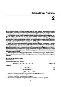
6.4 Asymptotic Convergence Rates We have observed cubic-like convergence in many of the tested problems. In Figure 2, we give edited printout from LIPSOL on the last several iterations for three Netlib problems: adlittle, beaconfd and stocfor3. We call the reader's attention to the column named Gap, representing the duality gap xT z + sT w. Since the equations xz = 0 and sw = 0 are the only nonlinear portion of the KKT system while the primal, dual and upper-bound feasibility conditions are all linear, the convergence rate of the duality gap usually dictates the asymptotic convergence rate of the whole residual vector. The last column is the total relative error and has no apparent correlation to the convergence rate of the residual vector. Residuals: Iter 10: Iter 11: Iter 12: Name:
Primal 9.22e-09 4.53e-11 2.11e-11 ADLITTLE
Dual 2.33e-11 9.31e-11 9.31e-11
U-bounds 0.00e+00 0.00e+00 0.00e+00
Gap 4.35e+00 5.91e-03 6.44e-10
TR-error 1.93e-05 2.61e-08 3.12e-14
Residuals: Iter 11: Iter 12: Iter 13: Name:
Primal 1.34e-06 4.45e-09 1.57e-10 BEACONFD
Dual 8.06e-08 4.80e-11 1.30e-11
U-bounds 0.00e+00 0.00e+00 0.00e+00
Gap 6.78e-01 1.34e-03 1.55e-10
TR-error 1.97e-05 3.84e-08 7.69e-14
Residuals: Iter 32: Iter 33: Iter 34: Name:
Primal 1.27e-05 2.32e-07 6.33e-08 STOCHFOR
Dual 3.23e-08 1.26e-10 2.97e-13
U-bounds 0.00e+00 0.00e+00 0.00e+00
Gap 4.09e-01 2.45e-03 2.09e-08
TR-error 1.02e-05 6.13e-08 9.59e-10
Figure 2: Examples of Cubic-like Convergence As can be seen from these examples, that cubic-like convergence not only happens for smaller problems such as adlittle and beaconfd, but also to large problems such as stocfor3, which 23
is the largest in the 95 Netlib problems in terms of problem sizes. However, on other problems cubic convergence is not observed up to the time when the algorithm terminates. In Figure 3, we present printout from LIPSOL for three problems: stair, pilot87 and ship08s. Residuals: Iter 12: Iter 13: Iter 14: Iter 15: Iter 16: Name:
Primal 1.34e-04 5.93e-05 1.64e-06 1.09e-05 1.59e-10 STAIR
Dual 5.24e-07 6.76e-08 1.78e-10 4.42e-15 2.98e-15
U-bounds 0.00e+00 0.00e+00 8.88e-16 1.26e-15 1.26e-15
Gap 4.29e-01 6.38e-02 7.64e-04 1.36e-08 1.36e-15
TR-error 1.69e-03 2.51e-04 3.02e-06 4.47e-08 6.55e-13
Residuals: Iter 32: Iter 32: Iter 34: Iter 35: Iter 36: Iter 37: Iter 38: Name:
Primal 1.86e-07 5.26e-08 1.94e-08 3.72e-09 9.29e-10 9.27e-10 2.21e-09 PILOT87
Dual 3.16e-11 9.49e-12 3.79e-12 3.07e-12 3.81e-12 4.82e-12 3.01e-12
U-bounds 5.07e-08 1.43e-08 5.28e-09 1.00e-09 2.03e-10 4.59e-11 1.65e-12
Gap 2.05e-02 5.86e-03 2.04e-03 4.29e-04 1.32e-04 2.07e-05 1.82e-06
TR-error 6.75e-05 1.93e-05 6.69e-06 1.41e-06 4.35e-07 6.79e-08 5.99e-09
Residuals: Iter 12: Iter 13: Iter 14: Name:
Primal 7.31e-05 2.12e-07 1.56e-11 SHIP08S
Dual 8.61e-11 9.17e-11 9.85e-11
U-bounds 0.00e+00 0.00e+00 0.00e+00
Gap 9.25e+01 3.05e-01 3.88e-07
TR-error 4.72e-05 1.56e-07 2.13e-13
Figure 3: Examples of Quadratic, Linear, and "Big bang" Convergence The convergence rate appears to be quadratic for stair and linear for pilot87, which is a well-known, ill-conditioned and di�cult problem. On the other hand, for ship08s, the convergence rate appears, surprisingly but pleasantly, to be even faster than cubic. It looks like that after a "big bang" iteration, the last iterate just drops into the optimal facet so the algorithm terminates right away.
7 Concluding Remarks In this paper, we provided intuitive motivations to some infeasible-primal-dual interior-point methods as perturbed and damped Newton's method. We described major steps in implementing an interior-point code for large-scale linear programming. We also discussed in detail a technique for stabilizing Cholesky factorization in the context of interior-point algorithms with mathematical justi cation. Our implementation was carried out under the MATLAB environment. Yet it is still su�24
ciently fast for large-scale problems and comparable in performance with a good Fortran code. The software package resulted from our implementation is called LIPSOL. LIPSOL is free software and available from the internet sites: http://pc5.math.umbc.edu/~yzhang/lipsol/ ftp://ftp.math.umbc.edu/pub/zhang/lipsol/v0.3/
where the rst is the LIPSOL Web page and the second an anonymous FTP site. In addition to providing an economic means for solving relatively large-scale linear programs, LIPSOL can be a convenient tool for both research and teaching. For more details on LISPOL, we refer readers to the User's Guide for LIPSOL [20] available in the aforementioned sites for LIPSOL distribution.
Acknowledgment This paper has directly bene ted from the works of a number of people to whom I am very grateful. The sparse Cholesky package developed by Esmond Ng and Barry Peyton. including the minimum-degree ordering subroutines by Joseph Liu, was used to construct MEX- les that forms the computational engine of LIPSOL. We received kind permission from Irv Lustig, Roy Marsten and David Shanno for using their system OB1 version 5.0 in our numerical experiments. A Fortran subroutine originally written by Alan Weiser was modi ed and used in LIPSOL to convert MPS les into MAT les. During the development of LIPSOL, I received programming assistance from Detong Zhang and valuable feedbacks from Stephen Wright.
References [1] E. D. Andersen, J. Gondzio, C. M�esz�aros and X. Xu. Implementation of interior-point methods for large-scale linear programming. Technical Report 1996.3, Logilab, HEC Geneva,Section of Management Studies, University of Geneva, Switzerland, 1996. [2] I. C. Choi, C. L. Monma and D. F. Shanno. Further development of a primal-dual interiorpoint method. ORSA J. on Computing, 2(1990) 304-311. [3] D. M. Gay. Electronic mail distribution of linear programming test problems. Mathematical Programming Society COAL Newsletter, No. 13 (Dec., 1985) 10-12. [4] J. Gondzio. Multiple centrality corrections in a primal-dual method for linear programming. Computational Optimization and Applications. To appear. 25
[5] N. Karmarkar. A New Polynomial{time Algorithm for Linear Programming. Combinatorica 4 (1984) 373{395. [6] M. Kojima, S. Mizuno, and A. Yoshise. A primal-dual interior point method for linear programming. In Nimrod Megiddo, editor, Progress in mathematical programming, interiorpoint and related methods, pages 29{47. Springer-Verlag, New York, 1989. [7] M. Kojima, N. Megiddo, and S. Mizuno. A primal-dual infeasible-interior-point algorithm for linear programming. Mathematical Programming 61 (1993) pp.263-280. [8] J. W. Liu, E. G. Ng and B. W. Peyton. On nding supernodes for sparse matrix computations. SIAM J. Matrix Anal. & Appl. 1 (1993) 242-252. [9] I. J. Lustig, R.E. Marsten, and D.F. Shanno. Computational experience with a primal-dual interior point method for linear programming. Linear Algebra and Its Applications, 152 (1991) 191{222. [10] I. J. Lustig, R.E. Marsten, and D.F. Shanno. On implementing Mehrotra's predictorcorrector interior point method for linear programming. SIAM J. Optimization 2 (1992) 435-449. [11] I. J. Lustig, R.E. Marsten, and D.F. Shanno. Interior point methods for linear programming: Computational state of the art. ORSA J. on Computing, 6(1994) 1-14. [12] I. J. Lustig. Barrier algorithms for linear programming. Workshop on Computational Linear and Integer Programming, Fifth INFORMS Computer Science Technical Section Conference, Jan. 7 { 10, 1996, Dallas, Texas, USA. [13] S. Mehrotra. On the implementation of a primal-dual interior point method. SIAM J. Optimization 2 (1992) 575-601. [14] S. Mizuno, M. J. Todd, and Y. Ye. On adaptive step primal{dual interior{point algorithms for linear programming. Mathematics of Operations Research 18 (1993) 964-981. [15] L. L. Nazareth. Computer Solution of Linear Programs, Chapter 3. Oxford University Press, New York, Oxford, 1987. [16] J. M. Ortega and W. C. Rheinboldt. Iterative Solution of Nonlinear Equations in Several Variables. Academic Press, New York, 1970. 26
[17] R. A. Tapia, Y. Zhang, M. Saltzman, and A. Weiser. The predictor{corrector interior{point method as a composite Newton method. SIAM J. Optimization, 6(1996) to appear. [18] X. Xu, P. F. Hung and Y. Ye. A simpli ed homogeneous and self-dual linear programming algorithm. Technical Report, Dept. of Management Science, University of Iowa, Iowa City, Iowa, 1993. [19] Y. Zhang. On the convergence of a class of infeasible interior-point algorithms for the horizontal linear complementarity problem. SIAM J. Optimization, 4(1994)208-227. [20] Y. Zhang. User's Guide to LIPSOL. Technical Report TR95-19, Dept. of Mathematics and Statistics, University of Maryland Baltimore County, Baltimore, MD 21228, 1995. [21] Y. Zhang, and D. Zhang. On polynomiality of the Mehrotra-type predictor-corrector interiorpoint algorithms. Mathematical Programming 68 (1995) 303-318.
27
Appendix: Test Results for LIPSOL v0.3 Problem 25fv47 80bau3b adlittle a ro agg agg2 agg3 bandm beaconfd blend bnl1 bnl2 boeing1 boeing2 bore3d brandy capri cycle czprob d2q06c d6cube degen2 degen3 d 001 e226 etamacro ��f800 nnis t1d t1p t2d t2p
Table 2: Test Results for LIPSOL v0.3 (I)
Rows Cols Iter Residual Primal Objective CPU sec. 822 1571 25 2.60e-13 5.5018458883e+03 15.27 2263 9799 37 6.39e-09 9.8722419330e+05 76.11 57 97 12 3.12e-14 2.2549496316e+05 0.71 28 32 7 3.68e-09 -4.6475314219e+02 0.35 489 163 18 1.01e-09 -3.5991767273e+07 5.85 517 302 16 2.57e-10 -2.0239252353e+07 6.84 517 302 16 6.69e-12 1.0312115935e+07 6.91 306 472 17 8.58e-11 -1.5862801844e+02 2.86 174 262 13 7.69e-14 3.3592485807e+04 2.41 75 83 12 8.25e-13 -3.0812149846e+01 0.80 644 1175 26 8.90e-09 1.9776295714e+03 7.68 2325 3489 33 3.84e-13 1.8112365404e+03 39.87 351 384 21 3.04e-09 -3.3521356672e+02 6.21 167 143 18 1.67e-11 -3.1501872801e+02 2.52 234 315 18 8.08e-09 1.3730803987e+03 2.58 221 249 16 4.04e-09 1.5185098958e+03 2.34 272 353 20 5.39e-11 2.6900129139e+03 3.81 1904 2857 27 2.98e-10 -5.2263930249e+00 40.16 930 3523 31 5.96e-12 2.1851966989e+06 14.80 2172 5167 31 8.50e-12 1.2278421081e+05 86.28 416 6184 25 1.70e-11 3.1549166666e+02 38.54 445 534 14 1.29e-11 -1.4351780000e+03 4.61 1504 1818 20 2.65e-10 -9.8729399974e+02 60.33 6072 12230 53 2.90e-09 1.1266396043e+07 4384.76 224 282 21 1.17e-09 -1.8751929046e+01 3.20 401 688 28 4.23e-09 -7.5571523297e+02 6.13 525 854 25 5.62e-10 5.5567956497e+05 10.97 498 614 27 2.33e-09 1.7279106571e+05 5.88 25 1026 18 6.94e-10 -9.1463780919e+03 8.34 628 1677 15 3.38e-10 9.1463780925e+03 53.10 26 10500 22 1.07e-10 -6.8464293294e+04 106.72 3001 13525 20 3.17e-10 6.8464293295e+04 197.93
28
Table 3: Test Results for LIPSOL v0.3 (II) Problem forplan ganges gi�pin greenbea greenbeb grow15 grow22 grow7 israel kb2 lot maros maros-r7 modszk1 nesm perold pilot pilot4 pilot87 pilotja pilotnov pilotwe recipe sc105 sc205 sc50a sc50b scagr25 scagr7 scfxm1 scfxm2 scfxm3
Rows 162 1310 617 2393 2393 301 441 141 175 44 154 847 3137 688 663 626 1442 411 2031 941 723 976 92 106 206 51 51 472 130 331 661 991
Cols Iter Residual Primal Objective CPU sec. 421 20 6.17e-10 -6.6421896090e+02 4.29 1681 18 1.09e-10 -1.0958573613e+05 9.62 1092 20 1.46e-11 6.9022359996e+06 4.32 5405 44 3.24e-10 -7.2555248106e+07 83.28 5405 37 5.02e-09 -4.3022602396e+06 68.05 645 17 1.02e-09 -1.0687094129e+08 6.22 946 19 1.03e-09 -1.6083433648e+08 9.64 301 16 4.88e-10 -4.7787811815e+07 3.06 142 22 8.64e-13 -8.9664482186e+05 6.83 41 15 3.44e-09 -1.7499001299e+03 1.07 308 18 9.83e-10 -2.5264706056e+01 1.65 1443 32 8.10e-13 -5.8063743701e+04 17.58 9408 14 1.02e-09 1.4971851676e+06 439.51 1620 24 2.71e-12 3.2061972906e+02 6.95 2923 30 4.17e-09 1.4076036546e+07 25.64 1376 33 5.18e-12 -9.3807552782e+03 15.10 3652 34 8.63e-09 -5.5748972915e+02 152.53 1000 28 4.69e-09 -2.5811392559e+03 12.66 4883 38 5.99e-09 3.0171034740e+02 472.62 1988 30 1.20e-09 -6.1131364638e+03 29.16 2172 20 1.60e-13 -4.4972761882e+03 18.15 2789 36 1.54e-09 -2.7201075328e+06 18.65 180 9 8.63e-11 -2.6661600000e+02 0.91 103 10 1.46e-13 -5.2202061212e+01 0.61 203 11 6.38e-09 -5.2202061119e+01 0.87 48 10 2.52e-14 -6.4575077059e+01 0.49 48 7 9.44e-10 -6.9999999976e+01 0.38 500 16 3.05e-12 -1.4753433061e+07 2.19 140 12 5.62e-11 -2.3313898243e+06 0.81 457 18 5.20e-12 1.8416759028e+04 2.93 914 19 4.10e-11 3.6660261565e+04 5.76 1371 20 7.65e-11 5.4901254551e+04 8.72
29
Table 4: Test Results for LIPSOL v0.3 (III) Problem Rows Cols Iter Residual Primal Objective CPU sec. scorpion 389 358 14 4.16e-11 1.8781248228e+03 1.65 scrs8 491 1169 24 1.12e-11 9.0429695380e+02 4.58 scsd1 78 760 10 2.94e-11 8.6666666746e+00 1.23 scsd6 148 1350 12 6.43e-11 5.0500000078e+01 2.30 scsd8 398 2750 11 4.00e-11 9.0499999995e+02 4.05 sctap1 301 480 17 5.75e-13 1.4122500000e+03 2.03 sctap2 1091 1880 18 3.45e-09 1.7248071473e+03 7.21 sctap3 1481 2480 18 6.61e-14 1.4240000000e+03 9.56 seba 516 1028 20 1.62e-10 1.5711600003e+04 15.26 share1b 118 225 20 1.05e-10 -7.6589318575e+04 1.65 share2b 97 79 12 2.09e-09 -4.1573224024e+02 0.87 shell 537 1775 18 3.07e-09 1.2088253485e+09 4.41 ship04l 403 2118 12 7.48e-11 1.7933245380e+06 3.83 ship04s 403 1458 13 1.27e-09 1.7987146998e+06 2.96 ship08l 779 4283 15 2.25e-09 1.9090552133e+06 9.18 ship08s 779 2387 14 2.13e-13 1.9200982105e+06 4.96 ship12l 1152 5427 15 8.58e-09 1.4701879275e+06 11.63 ship12s 1152 2763 15 6.73e-09 1.4892361411e+06 6.21 sierra 1228 2036 16 1.31e-12 1.5394362184e+07 12.55 stair 357 467 16 6.55e-13 -2.5126695119e+02 5.06 standata 360 1075 16 3.60e-11 1.2576995000e+03 3.49 standgub 362 1184 16 7.83e-10 1.2576995007e+03 3.61 standmps 468 1075 24 3.98e-13 1.4060175000e+03 5.81 stocfor1 118 111 17 1.38e-11 -4.1131976219e+04 1.10 stocfor2 2158 2031 22 3.24e-10 -3.9024408538e+04 14.44 stocfor3old 16676 15695 34 9.59e-10 -3.9976783944e+04 176.49 truss 1001 8806 18 3.73e-10 4.5881584721e+05 22.85 tu� 334 587 23 2.39e-11 2.9214776512e-01 6.24 vtpbase 199 203 28 4.36e-13 1.2983146246e+05 3.37 wood1p 245 2594 20 1.12e-11 1.4429024116e+00 43.97 woodw 1099 8405 27 3.98e-11 1.3044763331e+00 42.31
30