VOL. 11, NO. 7, APRIL 2016
ISSN 1819-6608
ARPN Journal of Engineering and Applied Sciences ©2006-2016 Asian Research Publishing Network (ARPN). All rights reserved.
www.arpnjournals.com
SOLVING NON-LINEAR DAMPED DRIVEN SIMPLE PENDULUM WITH SMALL AMPLITUDE USING A SEMI ANALYTICAL METHOD M. C. Agarana1 and M. E. Emetere2 1
Department of Mathematics, Covenant University, Nigeria 2 Department of Physics, Covenant University, Nigeria E-Mail:
[email protected]
ABSTRACT In this paper, we present a semi analytical solution for a damped driven pendulum with small amplitude, by using the differential transformation method. We begin by showing how the differential transformation method applies to the non-linear dynamical system. The method transformed the differential equation governing the motion of the pendulum into its algebraic form. The results obtained are in good agreement with the solution in the literature. The results show that the technique introduced is easy to apply to such dynamical system. Keywords: semi analytical method, small amplitude, non-linear damped driven simple pendulum.
1. INTRODUCTION The purpose of this paper is to employ the differential transformation method to the second order linear ordinary differential equation associated with pendulum dynamics. Most of the other methods available to solve the governing equations of motion of pendulum are trial and error in nature, thereby making them computationally intensive [1]. The differential transform method is a numerical method which requires no linearization or discretization [3]. In this work, we considered a damped driven pendulum as dynamical system whose governing equation is a second order linear ordinary differential equation. We solve this governing equation using DTM. The dynamic effect of the angular displacement and angular driven force are estimated from the solution of the governing equation [7]. 2. BASIC DEFINITION With reference to the articles [1, 2, 3] the differential transformation of a function r(x) can be written as: �
=
�!
��
[
��
�
]
=
�
(2)
� � �� �!
[
�
��
�
c)
]
= = , ℎ
�
=
�
d)
�
e)
�� �!
��
= sin
, ℎ
=
�
�� � ��
��
± , ℎ �
, ℎ
+
, ℎ
, ℎ � � = �
, ℎ
�
�
=
=
= � �+� !
=
�
�� �!
� �
± � +
��
+
2.2 DTM on second order ODE DTM can be used for second order linear ordinary differential equations as follows [2, 11]: Given =
�
[
−
]
−
(4)
The differential transformation of (4), by applying the above properties, is as follows: + �
+
+ =
�
+
� �+
�+
=
[�
�
[�
−
−
+
+ �
� +
+ − �
− � ]
] (5)
(6)
Equation (6) is subject to initial condition R(0) = R0 = a1
Equation (2) can be written using (1), as: = ∑∞ �=
a) � b) �
(1)
where r(x) is referred to as the original function and R(t) is the transformed function. The Taylor series expansion of r(x) about x=0 is the differential inverse transform of R(t). This can be defined as follows: = ∑∞ �= �
2.1 Some operation properties of differential transformation Combining equations (1) and (2), we derive the following mathematical operations whose proofs can be found in [4] and [5]:
(3)
and �
= �
=
(7)
Equation (7) is referred to as a recursive formula.
4478
VOL. 11, NO. 7, APRIL 2016
ISSN 1819-6608
ARPN Journal of Engineering and Applied Sciences ©2006-2016 Asian Research Publishing Network (ARPN). All rights reserved.
www.arpnjournals.com The appropriate solution = ∑∞ �= �
�
(8)
is obtained by using equation (2) and (7). 2.3 The governing equation The equation of motion for damped driven pendulum mass m and length l is given as [7]: � � ��
+ �
�� ��
+
� �=
With its dimensionless form as: � � ��
��
+
��
+ � �=
cos
cos
∆
∆
(9)
w
(10)
is the angular driven force, while C
is the amplitude of the driving force. Q is the damping parameter. The right hand side terms represent acceleration, damping and gravitation respectively. The term on the right hand side is a sinusoidal driving torque [7, 14]. For small angle of displacement, ; Sin =
(11)
��
��
+
��
+� =
cos
(12)
∆
Let ∅ = �� , the phase of the driving force term (7) Then equation (3) becomes � ′′
+
�′
At equilibrium, �
=
�. .
+ �
=
cos ∅
=
= − �′
− �
= , �′
�
(19)
=−
(20)
3. APPLICATION OF DTM In this section, we will apply the discussed DTM to solve equations (5) and (6). We start by re-writing equation (5) and (6) in a standard form and take the differential transform (DT) as follows: �[� ′′
⇒
∴�
+
+
= − �′ +
=
− �
�
+
�+
�+
= −
[−
]
(21) +
+ �
�
+
+
−�
− �
With the initial conditions Y(0) = 0, Y(0) = -1
So equation (2) can be written as � �
� ′′
Subject to
where m is the mass of the pendulum bob, is the length of the string, is the angular displacement, is the dissipation coefficient, g is the acceleration due to gravity, t represents time,
Now when the pendulum is not at equilibrium , the value of will be outside the above range. For this paper, the three dimensions for this system represented by equation (9), are ∅, � �′. Also both ∅ � have been restricted to reside within –� �, � respectively, in order to simplify the result of the system (13). We also let q = 1/2 and a = 0. The dimensionless governing equation to be transformed, using DTM, becomes (i.e.� ≠
(13)
(22)
](23)
(24)
By using the recursive relation in (9) with ≥ , we obtain values for Y(2), Y(3), Y(4), …, as follows: [2,10]. For k=0; we have �
=
�
=
�
=
�
=
=
(25)
For k=1, we have,
(14)
[ −
− − ]=− ⁄
(26)
[ −
(− ⁄ ) − ] = − ⁄
(27)
[−
( ⁄ ) − (− ⁄ )] = − ⁄
(28)
For k=2, we have
Equation (4) becomes =
cos ∅
That is, = cos ∅ ⇒∅=9 + 9
In general 2n 90 , where n = 1, 2, 3,…
(15)
For k=3, we have (16) (17) (18)
And so on. Generally, for
+
= ,
= , , , , … we have
4479
VOL. 11, NO. 7, APRIL 2016
ISSN 1819-6608
ARPN Journal of Engineering and Applied Sciences ©2006-2016 Asian Research Publishing Network (ARPN). All rights reserved.
www.arpnjournals.com �
=
,− ,, ,−
, …,
(29)
The terms are given as: Y(n) = Y(n-1) x -1/n, Where
Y(0) = -1 and n = 1, 2, 3, …
(30)
�
= − +
−
�
= − +
−
+
+⋯= +
=
(41)
+ ⋯ = 1632
1 (42) 2
and so on. Now for the velocity; Differentiating equation (36), with respect to t, we have 3 2 2 3 / (0) 1 0 0 0 ...
/ (t) 1 2 t t 2 t 3 ...
That is,
(43) (44)
3 2 / (1) 1 2 ... 2 3 16 / (2) 1 4 6 ... 3 27 / (3) 1 6 18 ... 2 128 / (4) 1 8 24 ... 3 75 250 / (5) 1 10 ... 2 3
(31)
�=
So let
∴
=
= ∑∞ �= � = �
−
=− +
+
−
−
+
+
=− +
+
+
+
+⋯
−
+⋯
−
+
For t = 1, 2, 3, 4, 5,…, we have �
=
= − +
�
= − +9−
�
= − +
−
−
and so on. For the acceleration, we differentiate equation (44) with respect to t, we have; (50)
+ …
+⋯
+
+
+
+⋯= − +⋯=
+⋯=
(51)
/ / (1) 0 2 3 2 ...
(52)
/ / (2) 0 2 6 8 ...
(53)
/ / (3) 0 2 9 18 ...
(54) (55)
(32)
/ / (5) 0 2 15 50 ...
(56)
(33)
and so on. Truncation the values of the angular displacement, velocity and acceleration after the fourth terms, we have respectively;
(34) (35)
(36)
(37)
�
(49)
/ / (4) 0 2 12 32 ...
Equation (34) can now be written as, �. . �
(48)
/ / (0) 0 2 0 0 ...
�
+ �
(47)
�
= ∑�
(46)
/ / (t) 0 2 3t 2 t 2 ...
From equation (8), ∞
(45)
(38)
�
= −
�
=
�
(57)
=
�
=
�
= 1632
(58) (59) (60)
1 2
(61)
(39) (40)
4480
VOL. 11, NO. 7, APRIL 2016
ISSN 1819-6608
ARPN Journal of Engineering and Applied Sciences ©2006-2016 Asian Research Publishing Network (ARPN). All rights reserved.
www.arpnjournals.com / (1) 1
the increase in angular displacement becomes so pronounced and sharp. Also both angular velocity and angular acceleration increase as time increases, as we can see from Figure-2 and Figure-3. However Figure-4 compares the increase in angular velocity with the increase in angular acceleration: The Figure shows that, at any given time, the increase in angular acceleration is more than the increase in angular velocity. Similarly in Figure5, the increases in angular acceleration, angular velocity and angular acceleration are compared. We notice that increase in angular displacement was at a point less than increase in both angular velocity and angular acceleration, but from time t = 5, the increase in angular displacement becomes higher than that of both increase in angular velocity and angular acceleration. From equation (18), the phase of the driven force can be written generally as 2n 90 . But for the interval being considered in this paper, the phase of the driven force ∅ � 9 .
(62)
1 (2) 2 3 1 / (3) 9 2 /
(63) (64)
2 3 5 / (5) 54 6
/ (4) 25
(65) (66)
// (1) 1
(67)
// (2) 4
(68)
// (3) 11
(69)
// (4) 22
(70)
// (5) 37
(71)
4. RESULT DISCUSSIONS With the assumptions in place, the results obtained show that the angular displacement increases as time increases, within the range of time considered (t = 1, 2, 3, 4, 5). From Figure-1, it can be seen that the increase at the beginning was not very pronounced, but after t=4
100 90
Angular Displacement
80 70 60 50 40 30 20 10 0 -10 0
2
4
6
8
Time Figure-1. Angular displacement of the pendulum at various times.
4481
VOL. 11, NO. 7, APRIL 2016
ISSN 1819-6608
ARPN Journal of Engineering and Applied Sciences ©2006-2016 Asian Research Publishing Network (ARPN). All rights reserved.
www.arpnjournals.com 60 50
Angular Velocity
40 30 20 10 0 0
1
2
3
-10
4
5
6
7
Time
Figure-2. Angular velocity of the pendulum at various times. 40
Angular Acceleration
35 30 25 20 15 10 5 0 0
1
2
3
4
5
6
7
Time Figure-3. Angular acceleration of the pendulum at various times.
4482
VOL. 11, NO. 7, APRIL 2016
ISSN 1819-6608
ARPN Journal of Engineering and Applied Sciences ©2006-2016 Asian Research Publishing Network (ARPN). All rights reserved.
www.arpnjournals.com 100
Velocity/Acceleration
80 60 Angular Acceleration
40
Angular Velocity 20 0 1
2
-20
3
4
5
6
Time
Figure-4. Comparing the angular acceleration with the Angular velocity of the pendulum at various times. 100 90 80
Displ/Vel/Accl
70 60 50
Angular Velocity
40
Angular Acceleration
30
Angular Displacement
20 10 0 -10
0
2
4
6
8
Time
Figure-5. Comparing the angular acceleration with the Angular velocity angular displacement of the pendulum at various times. 5. CONCLUSIONS A non-linear damped driven simple pendulum with small amplitude problem was solved using differential transformation method (DTM). The obtained results are plotted on graphs and are in agreement with the ones in literature. Deductions are made from both the graphs and equations. The differential transformation method is an effective method for solving the type of problem being considered in this paper. It is also easy to apply.
REFERENCES [1] H. Abdel - Halim Hassan. 2008. Application to differential transformation method for solving systems of differential equations. Applied Mathematical Modeling. 32: 2552-2559. [2] S. O. Edeki, et al. 2014. A Semi-Analytical Method for Solutions of a Certain Class of Second Order Ordinary Differential Equations, Applied Mathematics. 5: 2034-2041.
4483
VOL. 11, NO. 7, APRIL 2016
ISSN 1819-6608
ARPN Journal of Engineering and Applied Sciences ©2006-2016 Asian Research Publishing Network (ARPN). All rights reserved.
www.arpnjournals.com [3] O.O. Agboola, et al. 2015. Solution of third order ordinary differential Equations using differential transform method, Global journal of pure and applied mathematics. 11(4): 2511-2517.
Pendulum with Small Displacement. International Journal of Physical Sciences. 10(2): 364-370.
[4] 4. A. Arikoglu and I. Ozkol. 2005. Solution of Boundary Value Problems for Integro-Differential Equations by Using Transform Method, Applied Mathematics and Computation. 168: 1145-1158. [5] Z. Odibat. 2008. Differential Transform Methods for Solving Volferra Integral Equations with Separable Kernels, Mathematical and Computer Modeling. 48: 1144-1146. [6] M. Thongmoon and S. Pusjuso. 2010. The Numerical Solutions of Differential Transform Method and the Laplace Transform Methods for a System of Differential Equations. Nonlinear Analysis: Hybrid Systems. 4: 425-431. [7] M. C. Agarana and O. O. Agboola. 2015. Dynamic Analysis of Damped Driven Pendulum using Laplace Transform Method. 26(3): 98-109. [8] R.Fitzpatrick. 2006. The Simple Pendulum. Farside. Ph. Uteas. edu/teaching/301/lectures/node40.html. [9] Dehui Qui, Min Rao, QirunHuo, Jie Yang. 2013. Dynamical Modeling and Sliding Mode Control of Inverted Pendulum Systems. International Journal of Applied Mathematics and Statistics. 45(5): 325-333. [10] G.D. Davidson. 2011. The Damped Driven Pendulum: Bifurcasion Analysis of Experimental Date. The Division of Mathematics and Natural Sciences, Reed College. [11] J. Biazar and M. Eslami. 2010. Differential Transform Method for Quadratic Riccati Differentia Equations. International Journal of Nonlinear Science. 9(4): 444447. [12] F. M. S. Lima and P. Arun. 2006. An Accurate Formula for the Period of a Simple Pendulum Oscillating Beyond the Small Angle Regime. AMJ Phys. 74: 892-895. [13] L. E. Millet. 2003. The Large – angle Pendulum Period. Phys. Teach. 41: 162-163. [14] M. C. Agarana and S. A. Iyase. 2015. Analysis of Hermite’s Equation Governing the Motion of Damped
4484