This is achieved by deducing potential feasible paths from knowledge of previous explorations, without re-exploring finished nodes and their descendants in the ...
Solving The Multi-Constrained Path Selection Problem By Using Depth First Search1 Zhenjiang Li† , J.J. Garcia-Luna-Aceves† ‡ Department of Computer Engineering, University of California, Santa Cruz Santa Cruz, CA 95064, U.S.A. Phone:1-831-4595436, Fax: 1-831-4594829 Email: {zhjli,jj}@soe.ucsc.edu ‡ Palo Alto Research Center (PARC), 3333 Coyote Hill Road, Palo Alto, CA 94304 †
Abstract An extended depth-first-search (EDFS) algorithm is proposed to solve the multi-constrained path (MCP) problem in quality-of-service (QoS) routing, which is NP-Complete when the number of independent routing constraints is more than one. EDFS solves the general k −constrained MCP problem with pseudo-polynomial time complexity O(m2 · EN + N 2 ), where E and N are the number of links and nodes of a graph respectively, and m is the maximum number of feasible paths maintained for each destination. This is achieved by deducing potential feasible paths from knowledge of previous explorations, without re-exploring finished nodes and their descendants in the process of the DFS search. One unique property of EDFS is that the tighter the constraints are, the better the performance it can achieve, w.r.t. both time complexity and routing success ratio. Analysis and extensive simulation are conducted to study the performance of EDFS in finding feasible paths that satisfy multiple QoS constraints. The main results show that EDFS is insensitive to the number of constraints, and outperforms other popular MCP algorithms when the routing constraints are tight or moderate. The performance of EDFS is comparable with that of the other algorithms when the constraints are loose.
1. Introduction Routing algorithms supporting QoS differentiation differ from conventional routing algorithms in that, in QoS routing, the path from the source to the destination needs to satisfy multiple constraints simultaneously (e.g., band1 This work was supported in part by the National Science Foundation under Grant CNS-0435522 and by the Baskin Chair of Computer Engineering at UCSC
width, reliability, end-to-end delay, jitter and cost), while in conventional routing, routing decisions are made based only on a single metric. QoS-related routing metrics, as well as the corresponding constraints associated with them, can be categorized into minimal (maximal) metrics and additive metrics. A typical minimal metric is bandwidth, for which the end-to-end path bandwidth is determined by the minimal residual bandwidth of the links along the chosen path. It is relatively easy to deal with a routing constraint on minimal metric, because all the links whose residual bandwidth do not satisfy the requirement can simply be dropped. However, it is well known that path selection subject to two or more independent additive metrics is NP-complete [8], which means that there is no efficient (polynomial) exact solution for the general k − constrained MCP (multiconstrained path) selection problem. There also exist multiplicative metrics, such as loss rate, in which the end-to-end path loss is equal to the product of the loss rates of all intermediate links. Multiplicative metrics can be translated into additive metrics, or vice versa, by taking logarithmic or exponential function respectively. Therefore, we only consider additive QoS metrics and constraints in this work. Amongst all MCP problems, routing subject to two constraints has drawn the most interest, which includes a special case - the restricted shortest path (RSP) problem, where the goal is to find the path that satisfies one constraint while optimizes another metric simultaneously. The MCP (with two constraints) and the RSP problems are not strong NP-complete in that there are pseudo-polynomial running time algorithms to solve them exactly, in which the computational complexity also depends on the values of link weight in addition to the network size [2]. However, their complexity is prohibitively high when the values of link weight become large. Based on the latter observation above, Chen and Nahrstedt [1] proposed to scale one component of the link weight
Cost
Cost
down to an integer that is less than d wcii·x e, where x is a pre-defined integer and ci is the corresponding constraint on the weight component wi . They prove that the problem after weight scaling is polynomially solvable by an extended version of Dijkstra’s (or Bellman-Ford) shortest path (SP) algorithm, and any solution to the latter is also a solution to the original MCP problem. The running time is O(x2 N 2 ) when the extended Dijkstra’s SP algorithm is used; and it is O(xEN ) when the extended Bellman-Ford SP algorithm is used, where E and N are the number of edges and nodes, respectively. Neve and Mieghem proposed TAMCRA [7], where k − shortest paths are kept at each node w.r.t. a cost function of link weight components, hoping that one of them will satisfy the routing constraints. TAMCRA has computational complexity O(kN log(kN ) + k 3 CE), in which C is the number of constraints. Obviously, the performance and complexity of this heuristic depends on the value of k. Better performance can be achieved with a larger k at the cost of more execution time. Another common approach to solving the MCP problem is to choose a good aggregation link-cost function based on the link weight components and the given constraints. Then any shortest path algorithm, such as Dijkstra’s or Bellman-Ford, can be used to compute the shortest path w.r.t. the aggregated link cost. Jaffe [2] was the first to use a linear link-cost function lu,v = αw1 (u, v) + βw2 (u, v), in which α, β ∈ Z + . Ever since, both linear aggregation functions and non-linear aggregation functions have been proposed to solve the MCP problem. Compared with RSP, the k−constrained MCP problem has received far less attention. If a scheduling algorithm (e.g., weighted fair queuing) is used, then queuing delay, jitter and loss rate can be described as a function of bandwidth, such that the original NP-Complete MCP problem can be reduced to a traditional shortest path routing problem [5]. However, this is not true for propagation delay and is only applicable to networks using specific scheduling mechanisms. Yuan [9] generalized the ideas of link-weight scaling and k − shortest paths routing as limited-granularity heuristic and limited-path heuristic, respectively, and also proposed an algorithm to solve the general k−constrained MCP problem based on an extended Bellman-Ford algorithm. The running time of Yuan’s algorithm is |X| · N E, where |X| is the size of the table maintained at each node, for the limited granularity heuristic; and it is x2 N E, where x is the number of paths maintained at each node, for the limited path heuristic. Again, the performance and computational overhead of Yuan’s heuristics depends on the number of possible values to which link weight can be scaled down, or the number of paths to maintain at each node. In this paper, we propose EDFS, an algorithm based on depth-first search, to solve the general k − constrained
A X B
A
I B
C
C
D
D
E (a)
E Delay
(b)
Delay
Figure 1. Incomparable paths in {D × C} MCP. EDFS has time complexity O(m2 ·EN +N 2 ), where m is the maximum number of non-dominated paths maintained for each destination. This performance is achieved by deducing potential feasible paths from knowledge of previous explorations without re-exploring finished nodes and their descendants. One unique property of EDFS is that the tighter the constraints are, the better the performance it can achieve. In particular, EDFS can achieve almost the same success ratio as an exact solution does (with exponential running time complexity), while having less running time than that of Dijkstra’s algorithm when the routing constraints are very tight. The rest of the paper is organized as follows. First we give the network model and notations we are using in our discussion, including necessary background information about QoS routing. Then the basic idea behind the EDFS algorithm is illustrated and the details are demonstrated by its pseudo-code. The time complexity and performance of our algorithm are analyzed and examined by extensive simulations, in which we show how EDFS solves multiple-constrained path selection problem efficiently and effectively. To conclude, we summarize our work at the end of this paper.
2. Network Model and Problem Formulation We model the network as a directed graph G = {V, L}. Here, V is the set of nodes and L is the set of links interconnecting the nodes. That is, for node u and v in V , the link lu,v is in L if u and v are directly connected in G. In our discussion, we assume that each link lu,v is associated with a link weight vector wu,v = {w1 , w2 ...wk }, in which wi is an individual weight component. Accordingly, any path from the source node to the destination node can be assigned a path weight vector w(p) = {w1p , w2p ...wkp }, where wip equals to the sum of the corresponding weight components of all the links in the path. It has been pointed out that only those non-dominated paths (or incomparable paths) need to be maintained in multi-constrained routing [6]. Path p is dominated by path
undiscovered
(1)
3. Extended Depth-First-Search Algorithm In depth-first search (DFS), edges (we use edge and link interchangeably) are explored away from the most recently discovered node v that still has unexplored adjacent outgoing edges. When all of v’s edges have been explored, DFS backtracks to explore unscanned edges leaving the node from which v was discovered. This process continues, until all the nodes that are reachable from the source are discovered. The edges of a directed graph can be sorted into four groups w.r.t. a DFS search on it: tree, backward, forward and cross edges. An edge lu,v is a tree edge if node v was first discovered by exploring lu,v , and the tree having all the tree edges is named a DF S tree. Link lu,v is a back edge
c 6
(1,2) d (3,2)
(3,5) c
2
6
(2,4)
e (4,3) (2,5)
(1,1) (1,2)
2 (2,4)
e (4,3) d
(5,2)
(3,2)
g
QoS routing consists of disseminating a consistent view of the network (including network topology and resource state information) to each router, and a QoS routing algorithm responsible for finding feasible paths from the source to each destination satisfying multiple constraints. In this paper, we only consider the later, and assume that there exists a link-state routing protocol that disseminates topology and resource information to all routers in a timely manner.
Loop detected (3,5)
(1,1)
a
(2)
lu,v ∈p
1
g
MCP: Given a directed graph G = {V, L}, where V is the set of nodes and L is the set of links. each link {lu,v ∈ L} is assigned a link weight vector wu,v = {w1 , w2 ...wk }. A corresponding constraint vector is given as C = {c1 , c2 ...ck }, the problem is to find a feasible path p from the source node s to the destination node t such that
1
a
A path is called non-dominated if it is not dominated by any other path. The concept of path domination allows us to restrict the computational complexity by maintaining only those non-dominated paths, because the capability of QoS provisioning from the source node to the destination node can be represented by the set of non-dominated paths. For example, Figure 1 (a) shows a set of points in {Delay × Cost} representing the incomparable paths between a source-destination pair when the link weights are cost and delay. In Figure 1 (a), the path weight represented by point X is dominated by B, which has shorter delay and less cost. However, there exists no clear better or worse relation between any two paths of {A, B, C, D, E}, because none dominates another. Any routing request falls in the feasible area (shadowed area I of Figure 1 (b)) can be supported by at least one of the incomparable paths. The MCP problem can be formally formulated as follows.
wip ≤ ci f or i = 1, 2...k X where wip , wi (u, v)
finished
f
i = 1, 2...k
discovered
b
≤
wip , f or
f
wiq
b
q if
(5,2)
(2,5)
7 h (3,3)
8
3
7
4
i (2,2)
j
5
(a) node 6 is exploring c
h (3,3)
3
4
i (2,2)
8
j
5
(b) node 6 is exploring e
Figure 2. Illustration of EDFS1 if lu,v leads u to a ancestor v in the DF S tree. Link lu,v is a forward edge if it connects u to a descendant v in the DF S tree. All other edges are cross edges. Based on the type of edge explored in DFS, we extend DFS into a multi-constrained path searching algorithm based on the following observations. Because a tree edge always leads to a previously discovered node ud , we can add the path from the source to ud , together with its capability (path weight, more specifically), into the routing table. Backward edges form cycles and the search proceeds beyond a node that is already in the tree, given that the metrics that we are considering are additive. A forward or cross edge always leads to a finished node uf , which means that: (a) all the descendants of uf have been discovered and finished in a previous exploration away from uf , and (b) one or more paths to uf and its descendants are already known, node uf is reached again because a new path pnew to node uf is used (we call pnew the active path). Therefore, nondominated paths to uf and its descendants can be deduced without exploring away from uf once more. Based on the observations above, we can tell if any improvement on existing paths can be achieved by using pnew . This is possible because routing metrics are additive, and paths are comparable by using the concept of path domination. Here we 1 (a): Detect loop (2,g,4,i,5,j,2) when exploring backward edge j. Find dominating path (1, b, 6, c, 2) to node 2 via cross edge c, ∆ = w(1, b, 6, c, 2) − w(1, a, 2) = (−1, −2). For each descendant of node 2, improve w(1, a, 2, f, 3) + ∆ = (6, 7) + (−1, −2) → w(1, b, 6, c, 2, f, 3) = (5, 5) f or 3; improve w(1, a, 2, g, 4) + ∆ = (8, 7) + (−1, −2) → w(1, b, 6, c, 2, g, 4) = (7, 5) f or 4; improve w(1, a, 2, g, 4, i, 5) + ∆ = (10, 9) + (−1, −2) → w(1, b, 6, c, 2, g, 4, i, 5) = (9, 7) f or 5. (b): Find incomparable path w(1, b, 6, e, 7) to node 7 via forward edge e, ∆ = w(1, b, 6, e, 7) − w(1, b, 6, d, 7) = (−2, 2). For node 8, the descendant of node 7, compute new incomparable path w(1, b, 6, d, 7, h, 8) + ∆ = (8, 7) + (−2, 2) → w(1, b, 6, e, 7, h, 8) = (6, 9).
Algorithm 1 Procedure EDFS and EDFS Visit 1: procedure EDFS(G, src) 2: for all u ∈ V do 3: u.color ← W hite 4: π(u) ← nil 5: end for 6: EDFS Visit(src) 7: end procedure
. π(u) is u’s predecessor
8: procedure EDFS V ISIT(u) 9: u.color ← Grey 10: p.push(u) . p is current active path 11: U pdateRouteEntry(u, p, w(p), dT able) 12: for all v ∈ Adj(u) do . explore adjacent edge lu,v 13: if v.color = W hite then 14: π[v] ← u 15: w(p) ← w(p) + wu,v 16: EDF S V isit(v) 17: w(p) ← w(p) − wu,v 18: else if v.color = Grey then 19: continue . loop, scan next adjacent edge 20: else if v.color = Black then . v is finished 21: w(p) ← w(p) + wu,v 22: p.push(u) 23: U pdateRouteEntry(u, p, w(p), dT able) 24: p.pop(u) 25: w(p) ← w(p) − wu,v 26: end if 27: end for 28: u.color ← Black 29: M ergeDescendant(π(u), u) 30: p.pop(u) 31: end procedure
have three possibilities. First, the active path pnew to the finished node uf is worse than any existing path pold for uf . In this case, EDFS just ignores pnew and operates as the basic DFS. Second, if pnew is an incomparable path from the source to uf , then we can expect that new incomparable paths may be found to the descendants of node uf by following pnew . Third, if the path pnew dominates (i.e. is better than) the path pold , then better path to node uf and better paths to its descendants can be obtained, if any. Algorithm 1 shows the main procedures of the extended version of depth-first search (EDFS), and Algorithm 2 defines the functions called by EDFS. As we can see, one new structure - the descendant table dT able is used to keep track of the descendants of each node in the processing of DFS searching, which enables us to deduce possible dominating or incomparable paths when meeting a finished node. Note that EDFS specified in algorithm 1, 2 actually is able to find a set of incomparable paths with different QoS provisioning capabilities for each node reachable from the source. With minor modification, EDFS can stop searching right after a feasible path to the specified destination was found satisfying the given routing request. Figure 2 illustrates the basic idea of EDFS, in which we show how EDFS detects a routing loop, and finds dominating or incomparable paths for finished nodes and their descendants without re-exploring away from the finished nodes. We assume that each link is associated with two weight components, and when exploring away from a node, the adjacent edges are scanned alphabetically. Nodes are
Algorithm 2 Function U pdateRouteEntry, U pdateDesctRoutes and M ergeDescendant 1: function U PDATE ROUTE E NTRY(dst, p, w(p), dT able) 2: if no path for dst then 3: insert p 4: else 5: for each existing path pi for dst do 6: if p worse than pi then 7: return 8: else if p better than pi then 9: U pdateDesctRoutes(dst, p, pi , dT able) 10: delete pi , insert p 11: else if p incomparable with pi then 12: U pdateDesctRoutes(dst, p, pi , dT able) 13: insert p 14: end if 15: end for 16: end if 17: end function 18: function U PDATE D ESCT ROUTES (u, pnew , pold , dT able) 19: for each node di ∈ desct[u] do 20: for each path pj for di beginning with pnew do 21: if pnew better than pold then 22: improve the existing path pj for di 23: else if pnew incomparable with pold then 24: compute new incomparable path for di 25: end if 26: end for 27: end for 28: end function 29: function M ERGE D ESCENDANT (dad, kid) 30: desct[dad].push(kid) 31: for each descendant di ∈ desct[kid] do 32: desct[dad].push(di ) 33: end for 34: end function
also colored white or black to distinguish that they are undiscovered or finished respectively, and double circled nodes are discovered but not finished yet. As seen in Figure 2, a routing loop can be easily detected whenever a grey node is re-visited via backward edges. A cross or forward edge leads the DFS search to a previously finished node uf . If the current active path pactive to uf is dominating or inf comparable with any existing path pold to uf , given that f routing metrics are additive, we can have new dominating or incomparable path pnew for each descendant d of uf by d replacing the subpath pold of the existing path pold for d f d active , and compute the corresponding with the active path pf path weight as follows. active ) − w(pold ) = w(pold w(pnew f )] d ) + [w(pf d
(3)
Here 0 +, −0 are normal addition and subtraction operations on vectors of real numbers.
4. Computational Complexity In this section, we obtain the worst case running time complexity of EDFS. In Algorithm 1, the loop on lines 2-5 of EDF S takes O(N ) time for initialization. The function EDF S V isit is called exactly once for each node u ∈ V , because EDF S V isit is invoked only on white
curve of the polynomial function O(EN + N 2 ). Because we do not limit the number of incomparable paths maintained for each node, this result actually confirms the work done by Kuipers and Mieghem [4], where they have shown that, in practice, the worst case under which the number of non-dominated paths grows exponentially large hardly happens. However, to guarantee that the running time is polynomially bounded, we must specify the maximum number of incomparable paths maintained for each node. It is again a trade-off between performance and complexity. In what follows, we assign m = 5 in all our simulation configurations unless it is specified otherwise. Simulation results show that this is sufficient to achieve satisfactory performance in most scenarios.
Compare with polynomial function O(EN + N2 )
8
10
6
Running time in seconds
10
4
10
2
10
0
10
Simulation time O(EN + N2 )
−2
10
0
1000
2000 3000 4000 Number of nodes ( E = 2 x N)
5000
5.1. Exploring with different sequences
Figure 3. Time complexity of EDFS nodes and the first thing it does is to paint the node Grey. During an execution of EDF S V isit, the loop on lines 12-27 of EDF S V isit is executed |Adj[u]| times, where |Adj[u]| Pis the number of adjacent outgoing edges of u. Because u∈N |Adj(u)| = Θ(E), the total cost of executing lines 12-27 of EDF S V isit is O(E). Therefore, within the loop on lines 12-27, function U pdateRouteEntry on line 23 is called at most O(E) times, while outside the loop on lines 12-27, the function U pdateRouteEntry and M ergeDescendant are called exactly once for each node because each node is painted Grey and Black only once. In Algorithm 2, the function U pdateDesctRoutes is called at most m times by U pdateRouteEntry, where m is the maximum number of non-dominated paths we maintain for each node. The nested loops on line 19-27 take O(mN ) time to update existing paths to each descendant of node u. Because the push and pop operation take constant time, the loop on lines 31-33 of M ergeDescendant costs at most time O(N ). Summarily, we have O(EDF S) = O(N ) + O(N ) + O(E · m · mN ) + O(N 2 ) = O(m2 · EN + N 2 )
5. Extensions to the Basic Algorithm
(4)
To verify the correctness of our analysis, we conduct simulations running EDFS on networks of different sizes ranging from 10 nodes up to 5000 nodes. The network topologies in the simulations are randomly generated graphs (pure random graphs with pr = 0.11, as described later), and we do not limit the number of incomparable paths maintained for each node. The number of constraints is three and the source-destination pairs of requests are randomly chosen from the network. From Figure 3 we can see that the simulation time samples of EDFS ”resembles” the
For a given network, the DFS tree can be different if we scan the outgoing links at each node with different orders. As a consequence, from the same source, we may have a different set of incomparable paths for each reachable node with a different exploring sequence of nodes. By executing EDFS multiple times with different exploring sequences and combining the results of them, we will find better or more incomparable paths for nodes reachable from the source. As we will see shortly, Only one to three runs of EDFS are sufficient to achieve nearly optimal solution when the routing constraints are tight, while three to five runs of EDFS are needed to achieve satisfactory performance when the constraints are loose.
5.2. Crankbacking If the constraints are known in advance, it is intuitive that we do not need to go further deeper when we detect that current active path has already violated the requirements. It follows immediately that we can either continue to scan the next unexplored outgoing edge of node u, or crankback to the predecessor from which u was first discovered when there is no outgoing edge of u we can use to extend the current active path. Based on our simulations, crankbacking has two effects on the performance of EDFS. First, it cuts down the running time of EDFS by orders of magnitude, especially when the constraints are tight. Secondly, the success ratio of EDFS can be improved significantly. Simulation results show that the increase of the success ratio can be as much as 8 to 10% even with only a single execution of EDFS. The reason is that crankbacking actually equals to guiding EDFS searching to avoid unnecessary exploration, from which considerable time is saved, and the feasible path is more likely to be discovered in the first place. As a result,
this also allows us to run more executions of EDFS with different exploring sequences within the same time limit, such that higher success ratio can be achieved.
18
6. Performance Evaluation 6.1. Performance comparison with 2 constraints Three topologies and corresponding results are chosen to present here from all topologies we simulated: ANSNET, Pure-random graph and Waxman graph. ANSNET (32 nodes and 54 links) is widely used by Chen and Nahrstedt of [1] and other researchers to study QoS routing algorithms. In pure-random graphs, the existence of the link between any two nodes is determined by a pre-defined constant probability {pr | 0 < pr < 1}. It is purely random in the sense that pr is independent of any other factors, such as the distance between the two nodes. However, this usually is not true because, in practice, the probability for two nodes at far apart to have a direct connection is much lower than that for two nodes close by. Waxman’s model takes this into account, in which the probability pr is defined as d pr = αe− βL , 0 < α, β < 1, where d is the distance between these two nodes and L is the maximal distance between any two nodes in the graph. For the Waxman and pure-random graphs used in simulation, the field size of the simulation is a 15 × 10 rectangle, and the number of nodes is determined by the Poisson distribution with modified parameter λA, where λ is the original intensity rate and A is the field size. All nodes are randomly distributed within the simulation field at randomly chosen positions. As the first step, we compare the performance of different MCP algorithms subject to only two constraints.
23 19
2
24
11
25
12
5.3. Sorting links When the time does not allow running EDFS multiple times, it is critical to decide which outgoing edge to explore first at each node u. It is preferable for the new active path (obtained after extending it with one outgoing edge of u) to have as large a margin for the given constraints as possible. However, this is hard to tell without actually searching into the network. To deal with this problem, we sort the outgoing edges of every node u w.r.t. a certain parameter, which we Q call the normalized margin (NM). N M = ki=1 (1− wic(p) ), i where p is the new active path after extending one outgoing edge of node u. The outgoing edge with the maximal N M is explored first. In our simulation, we find that a 3 to 5% increase of success ratio can be achieved when the number of EDFS we execute is small (1 to 3 runs). The performance improvement becomes negligible when EDFS is called more times because most of the possible exploration sequences are exploited in the first few runs.
22
21
10
1
20
8 3 7
9
27
15 26 13
14
4 16
5
31
28
29
30 6
17
32
Figure 4. ANSNET, 32 nodes and 54 links The MCP algorithms we use to compare with EDFS are CN (Chen and Nahrstedt [1]), KKT (Korkmaz, Krunz and Tragoudas [3]) and JSP (a variation of Jaffe’s algorithm: Dijkstra’s shortest path algorithm w.r.t. the aggregated link + w2 (u,v) ]). As we mencost function w(u, v) = [ w1 (u,v) c1 c2 tioned early, CN maps the original MCP problem into a scaled version, in which one of the link weight components is scaled down within the range of (0, x] by wi0 (u, v) = e. They prove that there exists polynomial solud wi (u,v)·x ci tion to the scaled version of MCP, and any solution to the latter is also a solution to the original MCP problem. The basic idea of KKT is to run Dijkstra’s SP algorithm w.r.t. a linear aggregation function of the two link weight compo0 nents {wu,v = wi + k ∗ wj , i = 1 or 2}, and the coefficient k is self-adjustable according to whether the algorithm can find a feasible path for a given request with current values of i and k. Another execution of Dijkstra’s shortest path algorithm is invoked with new i and k if no feasible path was found with current values. As the baseline, we also implement an exact solution, which has exponential running time, but can give all feasible paths for a given routing request. For ANSNET, the first link weight component is uniformly distributed in (0, 50], while the second is uniformly distributed in (0, 200]. For the pure-random and Waxman networks, both link components are uniformly distributed in (0, 20]. The performance of MCP algorithms is measured by the success ratio, which is defined as follows SR =
number of routing requests being routed number of total routing requests
(5)
We also record the running time for each of the algorithms under consideration. As the baseline, we take the running time of Dijkstra’s as one, then the running time of other algorithms is measured by their multiples of the baseline: Dijkstra’s shortest path algorithm. The results for ANSNET, pure-random and Waxman networks are presented in Tables 1, 2 and 3 respectively. The source and destination
Table 1. Success ratio (SR) and running time, ANSNET
KKT (Korkmaz’s alg.) JSP (Jaffe’s alg.), CN (Chen’s alg.) c1 ∼ unif [50, 65] c2 ∼ unif [200, 260] c1 ∼ unif [75, 90] c2 ∼ unif [300, 360] c1 ∼ unif [100, 115] c2 ∼ unif [400, 460] c1 ∼ unif [125, 140] c2 ∼ unif [500, 560] c1 ∼ unif [150, 165] c2 ∼ unif [600, 660]
Exact
SR time SR time SR time SR time SR time
0.2486 37.39 0.5078 37.76 0.7522 38.34 0.9438 39.35 0.9880 38.18
EDFS #1 #2 0.2480 0.2486 0.2893 (1) 0.8262 (3) 0.4966 0.5060 1.177 (2) 2.318 (4) 0.7352 0.7471 2.649 (3) 4.379 (5) 0.9048 0.9256 3.588 (3) 5.882 (5) 0.9602 0.9720 4.116 (3) 6.699 (5)
JSP
KKT
0.2422 1 0.4896 1 0.7224 1 0.9214 1 0.9714 1
0.2480 5.855 0.5052 5.31 0.7470 4.08 0.9388 2.263 0.9848 1.804
x=3 0.1890 11.91 0.3294 11.95 0.4460 12.11 0.5422 12.22 0.6142 12.37
CN
x = 10 0.2274 98.37 0.4522 99.01 0.6664 101.3 0.8580 102.3 0.9232 103.6
Table 2. Success ratio (SR) and running time, Pure-random pr = 0.11 (39 nodes and 75 links) c1 , c2 ∼ unif [10, 20], SR time c1 , c2 ∼ unif [20, 30], SR time c1 , c2 ∼ unif [30, 40], SR time c1 , c2 ∼ unif [40, 50], SR time c1 , c2 ∼ unif [50, 60], SR time
Exact
0.0985 37.08 0.3810 36.61 0.6715 42.12 0.9325 35.98 0.9880 37.56
EDFS #1 #2 0.0980 0.0985 0.1674 (1) 0.4892 (3) 0.3720 0.3805 0.5851 (1) 1.669 (3) 0.6105 0.6640 1.091 (1) 3.114 (3) 0.9100 0.9195 4.749 (3) 7.813 (5) 0.9670 0.9770 5.43 (3) 8.925 (5)
nodes are randomly chosen in all simulation configurations, and all the results presented here are averaged over 5000 randomly generated routing requests for different ranges of the routing constraints. For different ranges of constraints, the first row gives the success ratio (SR) and the second row gives the corresponding running time. For EDFS, the number in parenthesis indicates the number of executions of EDFS (with different exploring sequences). As we can see, CN generally performs well only when the x is large enough, configurations with small values of x lag far behind all other algorithms in all simulation scenarios. Extremely high computational complexity is the main drawback of CN and makes it infeasible in practice. Note that, in our implementation, we only choose w2 to be scaled down, and it turns out that the time complexity of CN is already far more expensive than the other algorithms. According to Chen and Nahrstedt [1], another run of the algorithm must be performed in which another weight component w1 is scaled down instead, if we cannot find a feasible path when w2 is scaled. The performance of CN can catch up by specifying larger x or invoking another execution with w1 being scaled down, as shown by the work done by Chen and Nahrstedt [1] and other researchers [3], at much higher cost of execution time. KKT seems to be the best when the constraints are very loose (when more than 90% routing requests are actually routable), which is mainly due to the self adaptation of the coefficient k in the linear aggregation function. Korkmaz et al [3] show that the worse case complexity of
JSP
KKT
0.0975 1 0.3655 1 0.6385 1 0.9075 1 0.9770 1
0.0985 4.882 0.3755 5.913 0.6635 4.665 0.9245 2.372 0.9845 1.722
x=3 0.0780 11.52 0.2405 11.61 0.3925 11.69 0.5925 11.83 0.7145 11.97
CN
x = 10 0.0920 94.71 0.3355 95.48 0.5880 96.47 0.8765 98.37 0.9650 99.58
their algorithm is bounded by log(B(E+N log(N )), where {B = N · max(wi (u, v)), i = 1 or 2, lu,v ∈ E}. However, in our experiments, we notice that the running time of the algorithm becomes unpredictable when the basic approximation proposed by Korkmaz et al cannot find a feasible path to a destination. The reasons for this are the following. When the constraints are tight, multiple calls to the Dijkstra’s shortest path algorithm must be made, until the proper coefficient k is found. The tighter the constraints are, the more calls we need to make. If no feasible path can be found by the basic KKT, two heuristic extensions will be invoked , for which the running time is no long bounded by logarithmic times calls to Dijkstra’s shortest path algorithm. This explains why KKT generally takes a long time to find a feasible path when the routing constraints are tight. Our algorithm EDFS outperforms all the other algorithms when the routing constraints are tight and moderate w.r.t. running time, success ratio SR or both. As noted before, KKT performs better when the routing constraints are very loose. One unique property of EDFS is that the tighter the constraints are, the better its performance becomes. Particularly, EDFS takes even less time than Dijkstra’s shortest path algorithm to achieve nearly optimal success ratio (compared with the exact algorithm) when the constraints are very tight. We attribute this to the three extensions we made to the basic EDFS algorithm, especially crankbacking. Although KKT performs better when the constraints are very loose, its running time can become unpredictable when the basic approximation does not work. More importantly,
Table 3. Success ratio (SR) and running time, Waxman Exact
0.1130 73.72 0.4665 74.63 0.8650 75.19 0.9920 75.2
EDFS #1 #2 0.1125 0.1130 0.2134 (1) 0.6156 (3) 0.4455 0.4625 0.8363 (1) 2.424 (3) 0.7930 0.8520 1.739 (1) 4.979 (3) 0.9800 0.9865 6.909 (3) 11.37 (5)
KKT can deal only with a 2 − constrained MCP, while EDFS can solve the general k − constrained MCP problem. We also note that, in all simulation configurations, it takes at least 10 times (up to 30 times) longer than EDFS for KKT SR to be comparable with that of EDFS when the constraints are very tight, while EDFS lags no more than 1.3% of SR behind KKT by using 7 times longer time than KKT does at most, when the constraints are very loose. Surprisingly, Dijkstra’s SP algorithm has good performance at the lowest cost (except when the constraints are very tight, EDFS takes less time than Dijkstra’s SP), even w.r.t. a simP wi (u,v) , with ple linear link cost function w(u, v) = ci which the gap of SR between Dijkstra’s SP and exact algorithm is no more than 6% in all configurations.
In this section, we investigate the performance of EDFS subject to three or more constraints. Two new metrics are used to measure the performance of EDFS, which were first introduced by Yuan [9]. The first metric is the existence percentage EP , which is defined as EP =
number of requests routed by exact algorithm number of total routing requests
(6)
EP actually equals to the success ratio of exact algorithm, and indicates how likely a feasible path can be found to meet the given request. Small EP means that it is difficult to find a feasible path for the given constraints. Secondly, competitive ratio CR is defined as CR =
number of requests routed by heuristic algorithm number of requests routed by exact algorithm
(7)
CR indicates how well a heuristic algorithm can work against the exact algorithm with the same EP . In what follows, we use ANSNET as the simulation topology yet with three weight components for each link, and each of them is uniformly distributed in (0, 20]. Different constraints are chosen such that the existence percentage varies from 0.06 to 0.98, then the corresponding competitive ratios of EDFS with one, three and five executions are measured and plotted respectively in Figure 5. For each point in Figure 5, we use routing requests (source and destination are randomly
KKT
0.1120 1 0.4410 1 0.8065 1 0.9755 1
0.1130 5.711 0.4615 5.885 0.8405 2.968 0.9870 1.721
x=3 0.9350 11.46 0.3130 11.58 0.5415 11.67 0.7130 11.83
CN
x = 10 0.1080 93.6 0.4050 94.49 0.7870 96.53 0.9675 98.21
0.95
0.9
0.85
0.8 0
6.2. Performance with multiple constraints
JSP
1
Competitive ratio of EDFS
α = 0.45, β = 0.25 (40 nodes and 95 links) c1 , c2 ∼ unif [10, 20], SR time c1 , c2 ∼ unif [20, 30], SR time c1 , c2 ∼ unif [30, 40], SR time c1 , c2 ∼ unif [40, 50], SR time
EDFS (1) EDFS (3) EDFS (5)
0.2
0.4 0.6 Existence percentage
0.8
1
Figure 5. CR of EDFS with 3 constraints chosen) with the same constraints over 2000 randomly generated ANSNET topologies (link weights are different for each topology). As we can see, EDFS again performs well when the constraints are tight. One execution of EDFS almost has 100% CR when EP is less than 25%, and three runs of EDFS is enough to achieve no less than 95% competitive ratio when the constraints are very loose. To study the impact of the number of constraints on the performance of EDFS, we also conduct two sets of simulations on ANSNET, with the number of constraints varying from two to eight. In the first set of simulations, constraints are chosen such that the existence percentages are low, which are between 0.21 and 0.33. While in the second set, the existence percentages are high, which are between 0.71 and 0.82. The results are shown in Figure 6 and Figure 7 respectively. Again, every point is the average of requests using the same constraints over 2000 different ANSNET topologies. As we can see from Figure 6 and Figure 7, when the EP s are low (tight constraints), one execution of EDFS can achieve no less than 98% competitive ratios for all numbers of constraints, while three executions of EDFS already can have almost 100% competitive ratios. When the
1.005
1
Competitive ratio of EDFS
Competitive ratio of EDFS
1
0.995
0.99
0.985 EDFS (1) EDFS (3) EDFS (5)
0.98
0.975 1
2
3
4 5 6 Number of constraints
7
8
9
0.95
EDFS (1) EDFS (3) EDFS (5)
0.9
0.85 1
2
3
4 5 6 Number of constraints
7
8
9
Figure 6. Low EP ∼ [0.21, 0.33], ANSNET
Figure 7. High EP ∼ [0.71, 0.82], ANSNET
EP s are hight (loose constraints), three executions of EDFS are enough to have about 98% competitive ratios when the number of constraints varies from 2 to 8. Another advantage of EDFS is that its performance is insensitive to the number of constraints. Both the CRs (competitive ratio) with high EP s and CRs with low EP s do not vary much with different number of constraints. This is superior to heuristics using link weight scaling or limited granularity heuristic approach, whose performance may drop drastically as the number of constraints increases, as shown by Yuan [9].
[2] J. M. Jaffe. Algorithms for Finding Paths with Multiple Constraints. IEEE Networks, 14:95–116, 1984. [3] T. Korkmaz, M. Krunz, and S. Tragoudas. An Efficient Algorithm for Finding a Path Subject to Two Additive Constraints. In Proceedings of the ACM SIGMETRICS, pages 318–327, 2000. [4] F. Kuipers and P. V. Mieghem. The Impact of Correlated Link Weights on Qos Routing. In Proceedings of IEEE INFOCOM, 2003. [5] Q. Ma and P. Steenkiste. Quality-of-Service Routing for Traffic with Performance Guarantees. In Proceedings of the IFIP Fifth International Workshop on Quality of Service, pages 115–126, May, 1997. [6] P. V. Mieghem and F. A. Kuipers. Concepts of Exact Qos Routing Algorithms. IEEE/ACM Trans. Netw., 12(5):851– 864, 2004. [7] H. D. Neve and P. V. Mieghem. TAMCRA: A Tunable Accuracy Multiple Constraints Routing Algorithm. Computer Communications, 23:667–679, 2000. [8] Z. Wang and J. Crowcroft. Quality-of-Sservice Routing for Supporting Multimedia Applications. IEEE Journal of Selected Areas in Communications, 14(7):1228–1234, 1996. [9] X. Yuan. Heuristic Algorithms for Multiconstrained Qualityof-Service Routing. IEEE/ACM Trans. Netw., 10(2):244–256, 2002.
7. Conclusion We present EDFS, where the key idea is to maintain the descendant table dT able to deduce possible dominating or incomparable paths to a finished node and its descendants, without exploring away from the finished node again. The running time of EDFS is polynomially bounded by O(m2 ·EN +N 2 ). We showed through extensive simulations that EDFS outperforms other popular MCP algorithms when the routing constraints are tight or moderate, and is comparable with them when the constraints are loose, and its performance is insensitive to the number of constraints. Another attractive aspect of EDFS is that the tighter the constraints are, the better the performance it can achieve, w.r.t. both time complexity and routing success ratio (running time is even less than that of Dijkstra’s algorithm when the constraints are very tight).
References [1] S. Chen and K. Nahrstedt. On Finding Multi-constrained Paths. In Proceedings of ICC’98, pages 874–879, June, 1998.