ITM Web of Conferences 13, 01016 (2017) CMES2017
DOI: 10.1051/itmconf/20171301016
Some Prototype Results of the Symmetric Regularized Long Wave Equation Arising in Nonlinear Ion Acoustic Waves Erdem IŞIK1, Hasan BULUT2, Sibel Şehriban ATAŞ2,* 1 2
Tunceli Vocational School, Munzur University, Tunceli, Turkey Faculty of Science, Department of Mathematics, Firat University, Elazig, Turkey Abstract. In this manuscript, we consider the Bernoulli sub-equation function method for obtaining new exponential prototype structures to th Symmetric Regularized Long Wave mathematical model. We obtain new results by using this technique. We plot two- and three-dimensional surfaces of the results by using Wolfram Mathematica 9. At the end of this manuscript, we submit a conclusion in the comprehensive manner.
1. Introduction In the recent years, the investigation of exact travelling wave solutions to nonlinear partial differential equations plays an important role in the study of nonlinear modelling physical phenomena. Also the study of the travelling wave solutions plays an important role in nonlinear science. A variety of powerful methods has been presented, such as Hirota’s bilinear method[1]. the inverse scattering transform [2], sine-cosine method [3], homotopy analysis method [4,5], variational iteration method [6-8]. We study different aspects of the Symmetric Regularized-Long-Wave equation (SRLW). The Symmetric Regularized-LongWave equation is a model for the weakly nonlinear ion acoustic and space-charge waves[9]. This equation was introduced by Seyler and Fenstermacher in[10]. Moreover, some important results have been submitted to the literature by various scientists [11,21] The paper is organized as follows: In section 2, we describe the Bernoulli SubEquation function method (BSEFM). In section 3, we consider the following Symmetric
*
Corresponding author:
[email protected]
© The Authors, published by EDP Sciences. This is an open access article distributed under the terms of the Creative Commons Attribution License 4.0 (http://creativecommons.org/licenses/by/4.0/).
ITM Web of Conferences 13, 01016 (2017) CMES2017
DOI: 10.1051/itmconf/20171301016
Regularized Long Wave equation [22] defined by
utt uxx uuxt uxut uxxtt 0.
(1) Moreover, in section 4 we give the physical interpretations and remarks of the solutions obtained by BSEFM. Also a comprehensive conclusion is given in section 5. 2. Fundamental Properties of the Method An approach to the mathematical models including partial differential equations will be presented in this sub-section of paper. The steps of the this technique which is partially new modified can be taken as follows [10]. Step 1. We consider the following nonlinear partial differential equation (NLPDE) in two variables and a dependent variable u ;
P ux , ut , uxt , uxx ,
0,
(2)
and take the travelling wave transformation
u x, t U ,
(3)
x ct ,
where c 0 . Substituting Eq.(3) in Eq.(2) yields a nonlinear ordinary differential equation (NLODE) as following;
N U ,U ,U ,
where U
0,
(4) 2
dU dU ,U , d d 2
U ,U
.
Step 2. Take trial equation of solution for Eq.(4) as following:
U and where
n
a F i 0
i
i
a0 a1F a2 F 2
F bF dF M , b 0, d 0, M
an F n ,
(5)
0,1, 2 ,
(6)
F is Bernoulli differential polynomial. Substituting Eq.(5) along with Eq.(6) in
Eq.(4), it yields an equation of polynomial
F s F s
F of F as following; 1F 0 0.
According to the balance principle, we can obtain a relationship between Step 3. Let the coefficients of system;
i 0, i 0,
(7)
n and M .
F all be zero will yield an algebraic equations
, s.
(8)
Solving this system, we will specify the values of
a0 ,
, an .
Step 4. When we solve Eq.(6), we obtain the following two situation according to d ;
2
b and
ITM Web of Conferences 13, 01016 (2017) CMES2017
DOI: 10.1051/itmconf/20171301016
1
1 M d E F b M 1 , b d , e b
(9a) 1
b 1 M 1 M E 1 E 1 tanh 2 F , b d , E . (9b) b 1 M 1 tanh 2
Using a complete discrimination system for polynomial, we obtain the solutions to Eq.(4) with the help of Wolfram Mathematica 9 programming and classify the exact solutions to Eq.(4). For a better understanding of results obtained in this way, we can plot two- and three-dimensional surfaces of solutions by taking into consideration suitable values of parameters. 3. Application When we consider the travelling wave transformation and perform the transformation
u x, t U , kx ct
which
c is constant non-zero in Eq.(1), we obtain
NLODE as following;
2 k 2 c 2 U ckU 2 c2 k 2U 0. When we consider to Eq.(5) and Eq.(6) for balance principle between
(10)
U and U 2 , we
obtain the following relationship between n and M ;
2M n 2.
(11)
This relationship gives us some new different complex travelling wave solutions for Eq.(1). Case 1: If we take as
n 4 and M 3 in Eq. (11), we can write following equations;
U a0 a1F a2 F 2 a3 F 3 a4 F 4 , U a1bF a1dF 3 2a2bF 2 2a2 dF 4 3a2bF 3 3a3dF 5 4a4bF 4 4a4 dF 6 ,
(12) (13)
and
U b 2 Fa1 4bdF 3 a1 3d 2 F 5 a1 4b 2 F 2 a2 12bdF 4 a2 8d 2 F 6 a2 9b 2 F 3a3 24bdF 5 a3 15d 2 F 7 a3 16b 2 F 4 a4 6
2
8
40bdF a4 24d F a4 , where a2
(14)
0, b 0, d 0 . When we put Eq.(12-14) in Eq.(10), we obtain a system of
algebraic equations for Eq.(13). Therefore, we obtain a system of algebraic equations from
3
ITM Web of Conferences 13, 01016 (2017) CMES2017
DOI: 10.1051/itmconf/20171301016
these coefficients of polynomial of F . Solving this system with the help of wolfram Mathematica 9, we find the following coefficients and solutions; Case 1a. For b d , it can be considered the following coefficients;
24 2dka0
a1 0, a2
, a3 0,
a0 (a0 16 a0 2 )
a4 12d 2 k 2 a0 16 a0 2 ,
(15)
a0 a0 16 a0 2
1 ), b c k (a0 16 a0 2 4
4 2k
.
Substituting these coefficients in Eq.(12) along with Eq.(9a), we obtain the following new exponential function solution for Eq.(1);
4 x t a0 16 a02
u1 x, t a0
24a0 d 2e
8 2
4 x t a0 4 2dk e
Ek
E
16 a02
2
,
(16)
a0 a0 16 a0 2 ,
where a0 , d , k are real constants and
500
8 2
.
u x,t
6
400 300 200 100
0
5
10
15
x
Figure 1. The 2D and 3D surfaces of Eq.(16) under the values of
a0 5, k 0.3, d 50, E 0.8, 10 x 10, 1 t 10 and t 6 for 2D surfaces.
4
ITM Web of Conferences 13, 01016 (2017) CMES2017
DOI: 10.1051/itmconf/20171301016
b d , it can be considered follows;
Case 1b. Another coefficients for Eq.(1) and for
2c 2k a0 , a1 0, a2 24d c 2 k 2 , a3 0, k c
(17)
c2 k 2 a4 48cd k , b . 2ck 2
When we regulate Eq.(12) under the terms of Eq.(9a,17), we find the other new exponential function solution for Eq.(1);
u2 x, t
2c 2k 48cd 2 k 24d ck , 2 ( ct kx ) k c ( ct kx ) E 2d 2cdk cke E e
where c, d , k are real constants and
(18)
c2 k 2 . ck 0.6
u x,t
50 40 30 20 10 20
10
10
20
30
under
the
40
x
10 20
Figure
2.
The
2D
and
3D
surfaces
of
Eq.(18)
values
of
c 5, k 0.3, d 50, E 0.8, 20 x 40, 1 t 1 , t 0.6 for 2D surfaces. Case 1c. Another coefficients to the Eq.(1) for
a0 a4
8b 2 c 2
b d , it can be considered as follows;
a2 , a1 0,
1 4b 2 c 2 48c 2 d 2 ,k 1 4b 2 c 2
48bc 2 d 1 4b 2c 2
c 1 4b 2 c 2
, a3 0, (19)
.
Considering these coefficients in Eq.(12) along with Eq.(9a,19), we gain other new complex exponential function solution to Eq.(1);
5
ITM Web of Conferences 13, 01016 (2017) CMES2017
u3 x, t
8b 2 c 2 d 2e
DOI: 10.1051/itmconf/20171301016
4 bc t x 2 2
1 4b c
4bde
de
2bc t x
2 bc t x
where b, c, d are real constants and
E b2 E
bE
2
1 1 4b2c 2
,
(20)
. u x,t
140 120 100 80 60 40 20 10
5
5
10
15
x
Figure 3. The 2D and 3D surfaces of real part of Eq.(20) under the values of
b 2, d 0.1, c 1.1, E 0.8, 10 x 10, 5 t 5 , t 0.1 for 2D surfaces. 4. DISCUSSION AND CONCLUSIONS
The solutions such as Eq.(16,18,20) obtained by using BSEFM are the new exponential function structures solutions for Eq.(1) when we compare with the paper submitted to the literature by [22]. It has been observed that all solutions have verified the Eq. (1) by using Wolfram Mathematica 9. To the best of our knowledge, the application of BSEFM to the Eq.(1) has not been previously submitted to the literature. The method proposed in this paper can be used to seek more travelling wave solutions of NLEEs because the method has some advantages such as easily calculations, writing programme for obtaining coefficients and so many. Eq.(18) can be rewritten as hyperbolic functions by using the fundamental properties of hyperbolic functions as follows;
u1 x, t
24d c 2 k 2 2c 2k 48cd 2 k , k c ct kx 2d 2 2cdk E kce ct kx Ee
c2 k 2 . When we consider the general ck properties of hyperbolic and exponential functions, we can rewrite u1 x, t solution in
where
c, d , k
are real constants
and
the form of hyperbolic function as following.
6
ITM Web of Conferences 13, 01016 (2017) CMES2017
DOI: 10.1051/itmconf/20171301016
24d c 2 k 2 2c 2k 48cd 2 k u1 x, t , 2 2 k c E E 1 sec h 2 T 1 sec h ( T ) 2cdk sec h(T ) sec h T ct kx c2 k 2 , 2cdk , E c2 k 2 . T 2 2 ck c k
References 1. 2. 3.
R. Hirota, The Direct Method in Soliton Theory. Cambridge Univ. Press, (2004). M.J. Ablowitz, P.A. Clarkson, Solitons, nonlinear evolution equations and inverse scattering, Cambridge: Cambridge University Press, (1991). A. M. Wazwaz, Travelling wave solutions for combined and double combined sinecosineGordon equations by the variable separated ODE method. Appl. Math. Comput, 177, 755-760 (2006).
4.
M. Dehghan, J. Manafian, A. Saadatmandi, The solution of the linear fractional partial differential equations using the homotopy analysis method. Z. Naturforsch, 65a, 935949 (2010).
5.
M. Dehghan, J. Manafian, A. Saadatmandi, Solving nonlinear fractional partial differential equations using the homotopy analysis method. Num. Meth. Partial Differential Eq., 26, 448-479 (2010).
6.
J. H. He, Variational iteration method a kind of non-linear analytical technique: some examples. Int. J. Nonlinear Mech, 34, 699-708 (1999).
7.
M. Dehghan, M. Tatari, Identifying an unknown function in a parabolic equation with overspecified data via He’s variational iteration method. Chaos Solitons Fractals, 36, 157-166 (2008).
8.
M. Dehghan, J. Manafian, A. Saadatmandi, Application of semi-analytic methods for the Fitzhugh-Nagumo equation, which models the transmission of nerve impulses, Math. Meth. Appl. Sci, 33, 1384-1398 (2010).
9.
Carlos Banquet Brango, The Symmetric Regularized-Long-Wave equation: Wellposedness and nonlinear stability. Physica, D(241), 125-133 (2012).
10. C. Seyler, D. Fenstermacher, A symmetric regularized-long-wave equation. Phys. Fluids 27, 4–7 (1984).
7
ITM Web of Conferences 13, 01016 (2017) CMES2017
DOI: 10.1051/itmconf/20171301016
11. G. K. Watugala, Sumudu Transform: A New Integral Transform to Solve Differantial Equations and Control Engineering Problems. International Journal of Mathematical Education in Science and Technology, 24, 35-43 (1993). 12. Y. Pandir, New exact solutions of the generalized Zakharov–Kuznetsov modified equal-width equation. Pramana journal of physics, 82(6), 949–964 (2014). 13. H. Bulut, H. M. Baskonus and F. B. M. Belgacem, The Analytical Solutions of Some Fractional Ordinary Differential Equations by Sumudu Transform Method. Abstract and Applied Analysis,(2013). 14. A. M. Wazwaz, The tanh method: solitons and periodic solutions for Dodd-BulloughMikhailov and Tzitzeica- Dodd-Bullough equations. Chaos, Solitons and Fractals, 25, 55-56 (2005). 15. C.S. Liu, A new trial equation method and its applications. Communications in Theoretical Physics , 45(3), 395-397 (2006). 16. C.S. Liu, Trial Equation Method to Nonlinear Evolution Equations with Rank Inhomogeneous: Mathematical Discussions and Its Applications. Communications in Theoretical Physics, 45(2), 219–223. 17. H. Bulut, Y. Pandir, H. M. Baskonus, Symmetrical Hyperbolic Fibonacci Function Solutions of Generalized Fisher Equation with Fractional Order. AIP Conf., 1558, 1914 (2013). 18. Y. Pandir, Y. Gurefe, U, Kadak, and E. Misirli, Classifications of exact solutions for some nonlinear partial differential equations with generalized evolution. Abstract and Applied Analysis, 2012, 16 pages, (2012). 19. Ryabov, P. N., Sinelshchikov, D. I., and Kochanov, M. B., Application of the Kudryashov method for finding exact solutions of the high order nonlinear evolution equations. Applied Mathematics and Computation, 218(7), 3965–3972 (2011). 20. Kudryashov, N. A., One method for finding exact solutions of nonlinear differential equations. Communications in Nonlinear Science and Numerical Simulation, 17(6), 2248–2253 (2012). 21. Lee J., and Sakthivel, R., Exact travelling wave solutions for some important nonlinear physical models. Pramana—Journal of Physics, 80(5), 757–769 (2013). 22. H. Bulut, H.M.Baskonus, E. Cuvelek, On The Prototype Solutions of Symmetric Regularized Long Wave Equation by Generalized Kudryashov Method. Mathematics letters, 1(2), 10-16 (2015).
8