ability to accurately and artifact-free image or predict multiples, as part of surface ... term) on the interpolated data, which we will call the model. The general form for these .... tinuation with sparseness constraints:, EAGE 67th Conference & Ex-.
Sparseness-constrained data continuation with frames: Applications to missing traces and aliased signals in 2/3-D Gilles Hennenfent, and Felix Herrmann University of British Columbia, Department of Earth and Ocean Sciences Summary We present a robust iterative sparseness-constrained interpolation algorithm using 2-/3-D curvelet frames and Fourier-like transforms that exploits continuity along reflectors in seismic data. By choosing generic transforms, we circumvent the necessity to make parametric assumptions (e.g. through linear/parabolic Radon or demigration) regarding the shape of events in seismic data. Simulation and real data examples for data with moderately sized gaps demonstrate that our algorithm provides interpolated traces that accurately reproduce the wavelet shape as well as the AVO behavior. Our method also shows good results for de-aliasing judged by the behavior of the (f − k)-spectrum before and after regularization.
Introduction Price as well as constraints on marine and land acquisitions typically preclude dense and equidistant spatial sampling. As a result, seismic imaging may endure adverse affects limiting the ability to accurately and artifact-free image or predict multiples, as part of surface related multiple elimination. In addition, systematic under-sampling along the spatial acquisition coordinates may also give rise to aliased data. Typically, data continuation approaches involve some sort of a minimization problem that aims to jointly minimize a quadratic distance to the data penalized by a functional (regularization term) on the interpolated data, which we will call the model. The general form for these minimization problems, where missing data lie on a regular grid, has the following form 1 x ˆ = arg min kP (d − Tx) k22 + λJ(x). x 2
(1)
In this expression, d represents the data on the interpolated grid with P the picking operator that restricts the full data vector to the acquired data according to dacq. = Pd; λ the regularization parameter balancing the emphasis of data misfit versus a priori information residing in the penalty term J(x) and T either a modeling operator such as the adjoint of the (linear/parabolic) Radon, the apex-shifted Radon or the de-migration/de-DMO operator [14, 13] or a generic orthogonal transform such as the Fast or Discrete Fourier Transform [10, 4, 11]. Since the null space of the picking matrix is not trivial (i.e. null(P) 6= Ø)), there is an infinitely large family of solutions which account for the data. Unfortunately, not all these solutions are physically acceptable. Regularization is a method of imposing additional information and thus fill the null space of P. The success of data regularization depends upon choices for the modeling/transform operator and the penalty term.
Data continuation with sparseness constraints Sparseness on the model x by means of the `1 -norm, kxk1 has widely been used in geophysics [10, 9] and corresponds to the ability to represent the full data with minimal-structure, i.e., with a sparse model vector. Recently, `1 -minimization has received a flare of interest in theoretical signal processing in the context of decompositions of signals in redundant dictionaries consisting of multiple transforms such as the Discrete Cosine and Fast Curvelet Transforms [12, 1, 2]. These approaches have proven to be very effective as long the data can be written as a superposition of a limited number of ’waveforms’ residing in the columns of T. In [7], we demonstrated that dictionaries consisting of directional 2-D Wavelet frames with Discrete Cosines represent a suitable combination for data continuation. Following [12], we define the augmented system with the two transforms and the corresponding model vector as T = [T1 · · · T2 ] with
x = [x1 · · · x2 ]T ,
(2)
where T1,2 represent inverse 2 or 3-D Curvelet and Discrete Cosine transforms, respectively. To exploit the sparseness in x, we solve Eq. 1 with J(x) = kxk1 using a block solver in combination with iterative soft thresholding [12, 3]. At each iteration, evaluation of ! 2 X m−1 ∗ m−1 m s Ti xi ) (3) + Tj (d − xj = Sλm xj i=1
for j = 1, · · · , 2 yields an approximate estimate for the coefficient vector x. For large enough number of iterations, the solution of Eq. 3 converges after M iterations, to the following minimization problem on the coefficients 1 ˜ = arg min kd − Txk22 + λkxk1 . x x 2
(4)
with λ = λM . The soft thresholding element-by-element operation corresponds to ( x − sign(x)λ |x| ≥ λ s Sλ (x) = (5) 0 |x| < λ. For T an orthonormal basis, soft thresholding solves the `1 problem (cf. Eq. 4) explicitely while [3] demonstrated that the above iterative scheme converges for redundant frames to the solution of Eq. 4. The above solver provides an alternative to
Sparseness-constrained data continuation with frames the widely used Iterated Re-weighted Least Squares (IRLS) [8] and has the advantage that the block solver is relatively simple and flexible with regard to following the convergence and setting the threshold.
0
As shown independently within both the seismic (see e.g. [10, 11, 14]) and image (see e.g. [5]) processing communities, Eq. 4 can simply be adapted to the situation of missing data by including the picking operator (6)
Offset (m) 0
2000
0.5
Time (s)
1 ˜ = arg min kP (d − Tx) k22 + λkxk1 , x x 2
-2000
1.0
which corresponds to replacing Eq. 3 by 1.5
s xm j = S λm
+ T∗j P(d − xm−1 j
2 X
! ) . Ti xm−1 i
(7)
i=1
In practice, we typically set M ≤ 100 while λm is decreased exponentially from λ1 = λmax to λM = λmin . The maximum threshold λmax corresponds to a threshold that approximately preserves 10 % of the energy of the acquired data while λmin is for noise-free data set close to zero, λnoise-free ≈ 0. For noisy min data, we set the threshold directly proportional to the standard deviation (σn ) of the noise, λnoisy min ∝ σn . For more details on the Curvelet transform refer to [7, 6] and the references therein. We illustrate the performance of our method with respect to missing data with moderately sized gaps and de-aliasing by means of a sequence of 2-D synthetic and 2-/3-D real examples. We use the Fast Curvelet Transform of CurveLab [2] in 2- and 3-D.
Examples Application to synthetic data: Our synthetic acquired 512 × 512 data with missing traces and Gaussian white noise (SN R = 0dB) is presented in Fig. 1. We show in Fig. 3 a window of the result of the sparseness-constrained interpolation carried out on the full dataset. For comparison, Fig. 2 shows the same window in the noisy acquired data with missing traces. Notice that our algorithm provides interpolated traces that accurately reproduce the wavelet shape as well as the AVO behavior. Moreover, as a by-product of the interpolation algorithm, the shot gather is denoised. Indeed, the sparsity-constraint not only helps to interpolate but also to find the significant frame coefficients of the noise-free image. Aliased data (Fig. 4) gives rise to a wrap-around effect for the (f − k) spectrum (see Fig. 5). To remove these aliasing effects, we apply our algorithm to interleave traces. The (f − k) spectrum of the sparseness-constrained interpolation result is presented in Fig. 6 and shows that our algorithm also performs for de-aliasing. Application to real data: For 2-D (512 × 256) real data, the selected windows are shown in Fig.’s. 7 and 8. Our interpolation algorithm performs well for this data. For 3-D real data (280x368 traces of 256 time samples), the results are even better as shown in Fig.’s 9, 10 and 11. In the 3-D case, the 3-D Curvelets pick up information from all (time, shot and receiver coordinates) coordinates which helps the interpolation process.
2.0
Fig. 1: Synthetic acquired data with missing traces and Gaussian white noise (512 traces of 512 time samples) - SNR = 0 dB.
Discussion and conclusions The success of our approach essentially derives from the parsimoniousness of curvelet frames with respect to seismic data. As such, simple (iterative) soft holding procedures on the coefficients, based on weights that depend on the magnitude of the coefficients only, suffice to effectively interpolate the missing data. Soft thresholding can be seen as a mask that mutes those regions in the data that with high probability do not correlate with the waveforms in the colums of the Dictionary (T). The method derives its robustness from the sparseness of the tranform vectors. This sparseness facilitates the interpolation and separates data from noise. Extension of our method to the full 3-D case, clearly shows to be beneficial because the curvelets pick up information on the wavefront from all three coordinate directions ensuring continuity throughout. So far, we assumed data to be caustic-free and the main challenge lies in extending the method to cases where there are caustics.
Acknowledgments The authors would like to thank the authors of CurveLab (Candes, Donoho, Demanet and Ying), M. Beyreuther and J.F. Paradis. The authors also would like to thank Western Geco for the 3-D dataset. This work was carried out as part of the SINBAD project with financial support, secured through ITF (the Industry Technology Facilitator), from the following organizations: BG Group, BP, ExxonMobil and SHELL. Additional funding came from the NSERC Discovery Grant 22R81254.
References [1] Cand`es, E. J., and Guo, F., 2002, New multiscale transforms, minimum total variation synthesis: Applications to edge-preserving image reconstruction: Signal Processing, pages 1519–1543. [2] Candes, E., Donoho, D., Demanet, L., and Ying, L., 2005, CurveLab: Fast Discrete Curvelet Transform.
Sparseness-constrained data continuation with frames 1300 0.4
1400
Offset (m) 1500 1600
1700
1800
1300 0.4
0.5
Time (s)
Time (s)
1800
0.6
0.7
0.8
0.7
0.8
0.9
0.9
Fig. 3: Window of the sparseness-constrained interpolation result.
Offset (m) 0
-2000
0
2000
0.5
Time (s)
1.0
1.5
2.0
Fig. 4: Aliased data (171 traces of 512 time samples)
−0.5 −0.4 −0.3 −0.2 −0.1 f
[3] Daubechies, I., Defrise, M., and de Mol, C., 2005, An iterative thresholding algorithm for linear inverse problems with a sparsity constrains: CPAM, 57, no. 11, 1413–1457. [4] Duijndam, A., Volker, A., and Zwartjes, P., 2000, Reconstruction as efficient alternative for least-squares migration:, in 70th Ann. Internat. Mtg Soc. of Expl. Geophys., 1012–1015. [5] Elad, M., Starck, J., Querre, P., and Donoho, D., 2005, Simulataneous Cartoon and Texture Image Inpainting using Morphological Component Analysis (MCA):. [6] Herrmann, F. J., and Verschuur, D. J., June 2005, Robust curveletdomain primary-multiple separation with sparseness constraints: Robust curvelet-domain primary-multiple separation with sparseness constraints:, EAGE 67th Conference & Exhibition Proceedings. [7] Herrmann, F. J., June 2005, Robust curvelet-domain data continuation with sparseness constraints: Robust curvelet-domain data continuation with sparseness constraints:, EAGE 67th Conference & Exhibition Proceedings. [8] Karlovitz, L., 1970, Construction of nearest points in the `p , p even and `1 norms: J. Approx. Theory, 3. [9] Oldenburg, D. W., Levy, S., and Whittall, K. P., 1981, Wavelet estimation and deconvolution: Geophysics, 46, no. 11, 1528–1542. [10] Sacchi, M., and Ulrych, T., 1996, Estimation of the discrete fourier transform, a linear inversion approach: Geophysics, 61, no. 04, 1128–1136. [11] Schonewille, M., and Duijndam, A., 2001, Parabolic radon transform, sampling and efficiency: Parabolic radon transform, sampling and efficiency:, Soc. of Expl. Geophys., 667–678. [12] Starck, J. L., Elad, M., and Donoho, D., 2004, Redundant multiscale transforms and their application to morphological component separation: Advances in Imaging and Electron Physics, 132. [13] Trad, D., Ulrych, T., and Sacchi, M., 2003, Latest views of the sparse radon transform: Geophysics, 68, no. 1, 386–399. [14] Trad, D. O., 2003, Interpolation and multiple attenuation with migration operators: Geophysics, 68, no. 6, 2043–2054.
1700
0.5
0.6
Fig. 2: Window of the synthetic acquired data with missing traces and Gaussian white noise.
Offset (m) 1500 1600
1400
0 0.1 0.2 0.3 0.4 0.5 −0.5
−0.4
−0.3
−0.2
−0.1
0 k
0.1
0.2
0.3
0.4
0.5
Fig. 5: Wrap-around effect in the (f − k) spectrum of the aliased data.
Sparseness-constrained data continuation with frames Source 50
−0.5
100
r
−0.4
ec e
iv e
−0.3
R
−0.2
f
−0.1 0
0
0.1 0.2 0.3
0.5 −0.5
−0.4
−0.3
−0.2
−0.1
0 k
0.1
0.2
0.3
0.4
0.5
Fig. 6: (f − k) spectrum of the sparseness-constrained interpolation result with wrap-around effect almost totally removed.
Time-axis
0.4
100
200
140
150
Trace # 160 170
180
Fig. 9: Acquired data with missing traces
190
100
ei ve
r
Source 50
ec R
0
100
Time-axis
Time sample #
50
150
100
200
Fig. 7: Window of the real data with missing traces.
Fig. 10: Sparseness-constrained interpolation result.
100 140
150
Trace # 160 170
180
Receiver 200
300
190
50
50
Time
Time sample #
100
100
150
200 150
Fig. 8: Window of the sparseness-constrained interpolation result.
250
Fig. 11: Section of the sparseness-constrained interpolation result.