Spatial and temporal variation of selected physical ...

Spatial and temporal variation of selected physical and chemical properties of soil

B. Usowicz, J.B. Usowicz

EDITED BY B. USOWICZ, R. T. WALCZAK

Lublin 2004

2

Centre of EC Excellence AGROPHYSICS Centre of Excellence for Applied Physics in Sustainable Agriculture QLAM-2001-00428

Reviewed by: Assist. prof. dr hab. Cezary Sławiński

ISBN 83-87385-96-4

© Institute of Agrophysics PAS, Lublin 2004

Edition: 250 copies

Project of cover and computer edition: Boguslaw Usowicz Printed by: ALF-GRAF, ul. Kościuszki 4, 20-006 Lublin, Poland

3

CONTENTS 1. INTRODUCTION .....................................................................................................5 1.1. Objective .............................................................................................................6 2. GEOSTATISTICAL METHODS ..............................................................................7 2.1. Introduction.........................................................................................................7 2.2. Regionalized Variable.........................................................................................8 2.3. Semivariogram ....................................................................................................9 2.4. Trend .................................................................................................................13 2.5. Standardized semivariogram .............................................................................14 2.6. Cross-semivariogram ........................................................................................15 2.7. Kriging ..............................................................................................................16 2.8. Cokriging ..........................................................................................................18 2.9. Fractal dimension ..............................................................................................20 3. METHODS AND OBJECTS OF THE STUDY......................................................21 3.1. Reflectometric method for soil moisture measurement.....................................21 3.2. Determination of thermal properties of soil ......................................................22 4. TEMPORAL VARIATIONS IN THE AGRO-METEOROLOGICAL DATA.......25 4.1. The data.............................................................................................................26 4.2. Wavelet transform.............................................................................................28 4.3. The results of wavelet transform.......................................................................32 4.4. Empirical Mode Decomposition .......................................................................37 4.5. The results of EMD...........................................................................................38 4.6. The Multitaper Method .....................................................................................49 4.7. The results of the Multitaper Method...............................................................50 5. STATISTICAL AND GEOSTATISTICAL ANALYSES OF TIME SERIES OF THE PHYSICAL VALUES AND PROPERTIES OF SOIL............................56 5.1. Field experiment ...............................................................................................56 5.2. Results of statistical analysis.............................................................................57 5.3. Results of correlation analysis ..........................................................................67 5.4. Analysis of soil moisture semivariograms ........................................................68 5.5. Analysis of the fractal dimension of soil moisture............................................69 5.6. Results of reciprocal correlation analysis..........................................................77 5.7. Results of cross-semivariance analysis .............................................................78

4 5.8. Estimation of soil moisture distributions with the methods of kriging and cokriging ...........................................................................................................86 5.9. Assessment of conformance of kriging and cokriging estimations ...................90 5.10. Conclusion......................................................................................................92 6. INVESTIGATION OF SPATIAL VARIABILTY ..................................................94 6.1. Field experiment ...............................................................................................94 6.2. Results of statistical analysis.............................................................................95 6.3. Results of correlation analysis ..........................................................................98 6.4. Results of geostatistical analysis .......................................................................99 6.5. Estimation and preliminary analysis of maps..................................................100 6.6. Conclusion ......................................................................................................105 6.7. Soil moisture in field transects ........................................................................106 6.8. Basic statistics of soil moisture .......................................................................109 6.9. Semivariance...................................................................................................109 6.10. Comparison of soil moisture values – measured and estimated with the kriging method ................................................................................................111 6.11. Soil moisture distribution maps ....................................................................112 6.12. Conclusion....................................................................................................114 7. GENERAL CONCLUSION ..................................................................................114 8. REFERENCES ......................................................................................................116

5 1. INTRODUCTION

Spatial and temporal variability of the natural environment is its inherent and unavoidable feature. Every element of the environment is characterized by its own variability, and at the same time each element affects one or more other elements of the environment. In recent years, special attention has been turned to environmental variation as a phenomenon that comprises processes leading to given physical, chemical or biological conditions [1-4,7,27,28,38,39,86-101,201232,329-365]. One of the kinds of variability in the natural environment is the variability of the soil environment [9-13,20,35,44,118-141,272,286-321,338]. The variability is related to the spatial and temporal variation of soil-forming factors and to human activity. At the same time, the natural and the anthropogenic components of the spatial and temporal variability of soil are not sufficiently identified, and – so far – the least known. To the latter we should assign, among other things, excessive compaction of soil within the arable layer and beneath it, resulting – as a side effect – from the application of agricultural machinery, which has a significant effect on the hydro-physical, thermal and air relations in soil [64, 105,170,253,289,388,403,416,442]. Likewise with the chemical properties of soil, including its reaction (pH) and cation-exchange capacity [399]. Consequences of the failure to consider the spatial variability of the soil environment, and therefore the conditions of growth and development of plants, may include irrational tillage (not adapted to the existing conditions), plant development below optimum, meaningful losses in crop yields, excessive costs of fertilization and liming of soil, long-term retention of chemical components in the soil and their release in the form of gases or salts etc., as shown by studies conducted, among others, in the USA, Sweden, Great Britain, Australia, and also in Poland [6,8,34,116,117, 124,150, 154,156,171,207,229, 247, 286,393-398,411,418,426]. To acquire better and deeper knowledge and understanding of the temporal and spatial variability of the physical, chemical and biological features of the soil environment, we should determine the causes that induce a given variability. The primary causes of the natural variability may be sought in the geomorphological form of the terrain (mountains, uplands, flat lands, valleys, faults, terraces, detrital fans, dunes, etc.), among the soil-formation factors, i.e. the climatic, hydrological or biological factors and their interactions, and in the differences in the lithology of the parent rock from which he soil was formed. The intensity of erosion, sedimentation and weathering processes may also affect the temporal and spatial variation of soil properties [222,311,355-360].

6

It should be emphasized that the study of the spatial variability of the physical and chemical properties of soil provides the very foundations for precision agriculture that is now being promoted and implemented in the most economically developed countries [212,246,251,444]. Types of soils (including their genesis and primary features) are documented on the national, regional or administrative unit scale by means of soil maps with various degrees of generalization [21,83-85,186,252,362,365,384,419], and – though to a lesser extent – with the help of data banks [113,131,172,381,382, 452]. These provide a basis for the formulation of conclusions concerning the greater or lesser variability of soils within a given area [209,214,222,392399,416-419,446]. The variability of soil properties within an arable field, even though it exists [11,12,18,19,392], is often underestimated not only by farmers, but also by science. As a rule, the soil in a field is considered to be homogeneous, which permits the study of its physical and chemical parameters to be restricted to a single measurement point, and at the same time suggests the unification of all the applied tillage and other agricultural measures. This kind of approach causes that in the field of studies on the spatial variability of soil properties, conducted so far in Poland, there have been no significant research publications. The least known is the spatial variability of the properties of soil environment in the sense of mathematical-physical description and, moreover, the natural and anthropogenic components of the spatial variability of soils are not sufficiently distinguished [166,282,400,425]. Among the features of soil we can distinguish those relatively stable (little changing with time) and those of a more dynamic character which change with the occurrence of certain external factors (soil tillage, meteorological conditions). Relatively stable features of soil include its texture and mineral composition; examples of those variables in time are the soil pH or organic matter content; an example of a feature with strong dynamics is the soil moisture content. 1.1. Objective The objective of this work was to investigate and describe the spatial and temporal variability of selected physical and chemical properties of soil, determination of the extent of the variability and its significance in the soil environment using geostatistical methods and time series analysis.

7 2. GEOSTATISTICAL METHODS

2.1.Introduction The processes of mass and energy exchange taking place in soil are dynamic processes. This is affected primarily by the soil itself – a dispersive and multiphase medium – as well as by plants and the meteorological conditions. Actual soil objects studied under natural conditions are conveniently treated as systems connected to the environment that can be described by means of suitable functions of time or as systems being functions of time and spatial coordinates. With the physical structure of the systems studied not fully known (usually), their responses and contacts with the environment (inputs, outputs) can be analyzed in terms of static random processes, or treated as a form of interrelationship of random fields [36-75,127-137,145-185,199,236-285,404]. Statistical methods extensively used for the description of soil objects pre-assume that observations are independent from one another, which hinders their accurate description and analysis. In environmental studies we deal with observations which, by their very nature, are dependent on one another. The dependence is interesting as such (from the cognitive point of view) [17-22,142,144,204,213,288,319,364,368,369384,389,405-457]. In such a case, the chosen methods of random field analysis which, among other things, constitute the foundations for the mathematical apparatus of geostatistics, have a fundamental importance for the study of variation of soil parameters. As we are aware, our knowledge on a phenomenon or on the features studied with respect to a medium is fragmentary, as it relates to areas or, rather, points that have been sampled [9,24-85,322-379]. What we do not know is what actually happens in between the measurement points. The need to acquire knowledge on those areas resulted in the emergence of a new branch of science – geostatistics. Most of the features of the natural environment show continuity. The study of the physical properties of soil can be conducted with the help of classical statistics, using for the purpose the distribution function and the relevant statistical moments, or with the help of the autocorrelation function on which geostatistics is based. However, when we use classical statistics, we leave out information concerning the space from which data have been collected, and the data is irretrievably lost. On the other hand, basing on classical statistics we can solve the problem of sample population required for the determination of a given feature with specific accuracy. Geostatistics, which bases on observations that are similar within a certain proximity, indicates that they have to be mutually

8

correlated [315,345]. It represents a methodology that permits the spatial or temporal analysis of correlated data. Its basic tool is variogram analysis which involves the study of the variogram function of a specific variable physical value or of a soil property under study. The variogram function, with its specific parameters (nugget value, threshold and correlation range), presents the behaviour of the variable under study, called the “regionalized variable” [75,136,137,225, 426], and thus permits the formulation of conclusions concerning areas that are not represented by any measurement data [46, 53,57,62,63,70,126,159,179,190, 205, 214,377]. The concept of mathematical description of natural structures characterized by geometric heterogeneity of linearity or surface may be conducted with the help of the fractal theory [6,8,10,14-16,346-352]. The fundamental concept in this theory is the concept of the fractal dimension D [29,42,43,161,167,176,220,221] which expresses the effective geometric dimension of linearity, surface or volume of a structure under study. According to the fractal theories, the value of D is a global value and therefore characterizes the whole object studied [275-278,291-297, 383, 396]. The value may assume values within the range of 1 ≤ D ≤ 2 for linear sections and 2 ≤ D ≤ 3 for surfaces, and can be interpreted in terms of spatial organisation of the feature or process under study, i.e. it provides information on how far the feature/process is determined or has a random character. Comprehensive study of the dynamics and correlation of many physical properties of soil and the close-to-ground layer of atmosphere combined is now possible thanks to the existence of suitable methods of measurement, availability of automatic data acquisition and analysis systems, and the adaptation of geostatistical methods and the fractal theory to the temporal and spatial analysis of data variability. 2.2. Regionalized Variable A basic concept in geostatistics is the regionalized variable introduced by G. Matheron [225]. The variable, distributed in space, forms a certain random field and is used for the description of phenomena occurring within a specific zone. The duality of the regionalized variable is manifest in two aspects – deterministic (structured) and random (erratic) after Pannatier [280,281]: “- The structured aspect is related to the overall distribution of the natural phenomenon, - The erratic aspect is related to the local behavior of the natural phenomenon.

9

The formulation of a natural phenomenon must take this double aspect of randomness and structure into account. A consistent and operational formulation is the probabilistic representation provided by Random Functions. A Random Function is a set of Random Variables {Z(x) | location x belongs to the area investigated} whose dependence on each other is specified by some probabilistic mechanism. It expresses the random and structured aspect of a natural phenomenon in the following way : - Locally, the point value z(x) is considered as a Random Variable. - This point value z(x) is also a Random Function in the sense that for each pair of points xi and xi +h, the corresponding Random Variables Z(xi) and Z(xi +h) are not independent but are related by a correlation expressing the spatial structure of the phenomenon.” 2.3.Semivariogram As has been mentioned earlier, in studies on the soil environment we deal with observations that are mutually correlated [2,47,48,60,61,66,126,129,138,140]. Statistical methods assume that observations are independent from one another, which hinders the accurate description and analysis. We know that our knowledge on the processes studies is fragmentary as it relates to areas, or rather to points that have been observed. We do not know what happens within the areas in between the observations [70,90,94,96-120,248-268,315,325,387,436-450]. Acquisition of knowledge about those areas is in the focus of interest of numerous branches of science, including agrophysics [392-400,419]. The probability, confirmed by numerous observations, that next to a point with a specific value of a certain variable there are points with similar values of that variable indicate that the values must be mutually correlated. The basis for the calculation of data so correlated is the method of variogram function analysis, and more specifically a half of the expected value of differences of the value Z(x) of the variable in point x and value Z(x+h) in a point removed by the vector h. The semivariogram presents therefore the spatial or temporal behaviour of a given variable which is also called the “regionalized” variable. The variable has its random aspect which accounts for local irregularities, and its structural aspect which reflects the overall tendency or trend of the phenomenon (trend) [122]. Analysis of such a variable consists in the identification of the structure of variability. Three stages can be identified in the analysis: preliminary examination of collected data and evaluation of basic statistics, calculation of empirical variogram of the regionalized variable under analysis, and fitting a mathematical model to the

10

course of the empirical variogram. This requires the knowledge of the first two statistical moments of the random functions ascribed to a given phenomenon: the first moment (the mean) [281],

E [Z ( x )] = m( x )

(1)

and the second (variance, covariance, semivariogram – semivariance)

{

}

Var{Z (x )} = E [Z ( x ) − m( x )] . 2

(2)

If the random variables of Z(x1), Z(x2) have variance, they also have covariance which is a function of position x1, x2: C (x1 , x 2 ) = E {[Z ( x1 ) − m (x1 )]⋅ [Z (x 2 ) − m( x 2 )]} = E {Z (x1 ) ⋅ Z (x 2 )}− m ( x1 ) ⋅ m (x 2 ) (3)

Semivariogram γ(x1,x2) is defined as a half of the variance from the difference of random variables {Z(x1)– Z(x2)} [281,424,425]:

γ ( x1 , x 2 ) = Var{Z (x1 ) − Z ( x 2 )} . 1 2

(4)

It is also required that the process under study be stationary, i.e. does not change its properties with a change in the beginning of the temporal or spatial scale. In the stationarity condition is met, the random function Z(x) is defined as a stationary function of the second order. Moreover, it is expected that [188, 189, 281]: - the expected value exists and does not depend on the position of x

E [Z ( x )] = m ,

∀x

(5)

- for each pair of random variables {Z(x), Z(x+h)} there exists covariance dependent only on the separation vector h

{

}

C (h ) = E Z ( x + h ) ⋅ Z ( x ) − m 2 ,

∀x

(6)

- the stationarity of covariance implicates the stationarity of variance and semivariogram

{

}

Var{Z (x )} = E [Z ( x ) − m] = C (0 ), 2

∀ x.

(7)

11

It can be shown that there is a correlation between covariance and the semivariogram [281]:

[{ } − [E {Z ( x + h ) }− 2 E{Z ( x + h ) ⋅ Z ( x )} + E {Z ( x ) }]

] [{

}

2C (h ) = 2 E{Z ( x + h ⋅ Z ( x ))} − 2m 2 = E Z ( x + h ) − m 2 + E Z ( x ) − m 2 2

2

2

]

2

2C (h ) = 2C (0) − 2γ (h ) C (h ) = C (0) − γ (h )

(8) - for all the values of vector h the difference {Z(x+h) – Z(x)} has finite variance and does not depend on x

γ (h ) = Var{Z ( x + h ) − Z ( x )} = 1 2

{

}

1 2 E [Z ( x + h ) − Z ( x )] , 2

∀x .

(9)

When the value of vector h equals zero, the value of semivariance is also equal to zero. The semivariogram is symmetrical with relation to h:

γ(h)=γ(–h).

(10)

The experimental semivariogram γ(h) for the distance h is calculated from the equation [124,191,267,281,323,380, 402,424]:

γ (h ) =

1 N (h ) [z (xi ) − z (xi + h )]2 ∑ 2 N (h ) i =1

(11)

where: N(h) is the number of pairs of points distant for each other by h. The equation illustrates the differentiation of deviations of the value of a given feature or physical value z from the equation of trend with relation to the distance between the measurement points. Three characteristic parameters are distinguished for the semivariogram: the nugget effect, the threshold, and the range. If the semivariogram is an increasing function beginning not from zero but from a certain value, the value is called the nugget effect. It expresses the variability of the physical value under study with a scale smaller than the sampling interval (it can also result from low accuracy of measurement). The value, reached by the semivariogram function, from which no further increase of the function is observed, (approximately equal to the sample variance) is called

12

the threshold or sill, while the interval from zero to the point where the semivariogram reaches 95% of the constant value is called the range. The last parameter expresses the greatest distance at which the values samples are still correlated. To semvariograms determined empirically, the following mathematical models are fitted [91, 280,281]: - The linear isotropic model describes a straight line variogram. Note that there is no sill in this model; the range A0 is defined arbitrarily to be the distance interval for the last lag class in the variogram. The formula used is [109]:

γ (h ) = C 0 + h C A  0   

(12)

- The spherical isotropic model is a modified quadratic function for which at some distance A0, pairs of points will no longer be autocorrelated and the semivariogram reaches an asymptote. The formula used for this model is: 3    h   h C + C ⋅ 1.5 − 0.5   γ (h ) =  0  A0  A0     C 0 + C

h ≤ A0

,

(13)

h > A0

- The exponential isotropic model is similar to the spherical in that it approaches the sill gradually, but different from the spherical in the rate at which the sill is approached and in the fact that the model and the sill never actually converge. The formula used for this model is: h   − A0 γ (h ) = C 0 + C ⋅ 1 − e   

h >0

(14)

- The Gaussian or hyperbolic isotropic model is similar to the exponential model but assumes a gradual rise for the y-intercept. The formula used for this model is: h  − 2 A γ (h ) = C0 + C ⋅ 1 − e 0 

2

   

h >0

(15)

where: γ(h) semivariance for internal distance class h, h – lag interval, C0 – nugget variance ≥ 0, C – structural variance ≥ C0, A0 – range parameter. In the case of linear model there is no effective range A – is set initially to the separation

13

distance (h) for last lag class graphed in the variogram. In the case of the spherical model the effective range A = A0. In the case of the exponential model the effective range A = 3A0 which is the distance at which the sill (C + C0) is within 5% of the asymptote. In the case of the Gaussian model, the effective range A = 30.5A0 which is the distance at which the sill (C + C0) is within 5% of the asymptote. When fitting a model to empirical semivariograms, the least squares method is most frequently used. 2.4. Trend In the regionalized variable we can distinguish the random or erratic component – ε(x), which covers local irregularities, and the structural component – m(x), which reflects the overall tendencies of the phenomenon (trends). The components are closely related to each other through the decomposition equation [71,122,424]:

z ( x ) = ε ( x ) + m( x )

(16)

Like above, analysis of such a variable consists in the identification of the structure of variability through examination of the collected data and evaluation of the basic statistics, calculation of the empirical semivariogram of the regionalized variable under consideration, and fitting a mathematical model to the course of the empirical semivariogram. It is also required for the process under study to be stationary, i.e. not to change its properties with a change in the beginning of a spatial or temporal scale. The existence of trends in a data set causes a change in the properties of the feature together with scale change. In such a case fulfilling the stationarity condition requires the removal of the trend – m(x) from the data set [114]:

ε ( x ) = z ( x ) − m( x ) .

(17)

For a linear run of values the trend equations are as follows:

m( x ) = a 0

m( x ) = a 0 + a1 x

m( x ) = a 0 + a1 x + a 2 x 2

(18)

14

When we have a surface trend with x, y coordinates, the trend equations are as follows:

m( x , y ) = a 0

m( x, y ) = ax + by + c

(19)

m( x, y ) = ax 2 + by 2 + cxy + dx + ey + f

where: a, a0, a1, a2, b, c, d, e, f – parameters. After the elimination of the trend from the data set, the resultant random or erratic component should be characterized by the mean value of zero and by finite variance. The empirical semivariogram − γ(h) for the distance h is calculated from the equation:

γ (h ) =

1 N (h ) [ε (xi ) − ε (xi + h )]2 ∑ 2 N (h ) i =1

(20)

where:: N(h) is the number of pairs of points distant by h. The equation illustrates the differentiation of deviations of the values of a given features or physical value ε(xi) from the trend equation depending on the distance between the measurement points. 2.5. Standardized semivariogram Semivariance values calculated from the classical equation are sometimes so scattered that it is difficult to them a semivariogram model. Better model fit can be achieved through the standardization of the semivariogram γ s [281]:

γs =

γ (h ) . σ h =0 ⋅ σ h

(21)

In such a case we must additionally calculate the standard deviation of the random variable at the origin of vector h ( σ h = 0 ) and the standard deviation of the value of the random variable for a point distant by h ( σ h ).

15

2.6. Cross-semivariogram Regionalized variables are assigned to various physical properties of the soil medium. The variables are usually correlated with one another, to a lesser or greater degree. Assuming that the condition of stationarity of the second order is met, and that the values of variables z1 and z2 have cross-covariance defined as [123,193,230,407,434]:

C12 (h ) = E{Z1 ( x ) ⋅ Z 2 ( x + h )}− m1m2

(22)

C 21 (h ) = E{Z 2 ( x ) ⋅ Z1 ( x + h )}− m1m2

(23)

and

and cross-semivariogram as:

γ 12 (h ) = γ 21 (h ) = E{[Z1 ( x + h ) − Z1 ( x )]⋅ [Z 2 ( x + h ) − Z 2 ( x )]}, ∀x . 1 2

(24)

When m1 and m2 are the expected values E{Z1(x)} and E{Z2(x)} then, taking the above relations we can write the cross-semivariogram as:

2γ 12 (h ) = 2γ 21 (h ) = 2C12 (0) − C12 (h ) − C 21 (h )

(25)

The empirical cross-semivariogram − γ(h) for the distance h is calculated from the equation:

γ 12 (h ) =

1 N (h ) ∑ [z1 (xi ) − z1 (xi + h)] ⋅ [z 2 (xi ) − z 2 (xi + h)] 2 N (h ) i =1

(26)

where N(h) is the number of pairs of points with values of [z1(xi), z1(xi+h)], [z2(xi), z2(xi+h)], distant by h. When calculating the cross-semivariogram, the number of z1 and z2 values need not be even. Like in the semivariogram, in the crosssemivariogram three basic parameters are distinguished: the nugget, the sill, and the correlation range. Also, mathematical functions are fitted into empirically determined cross-semivariograms. The obtained mathematical functions of semivariograms and crosssemivariograms can be used for the spatial (temporal) analysis of autocorrelation or for the visualization, through estimation, of the physical value under

16

consideration in space with the kriging or cokriging methods [30-33,91,127-129, 200,281]. 2.7. Kriging Estimation of values in places where no samples have been taken can be conducted with the help of an estimation method called the kriging method [40,41,55,58,77,80,164,223,270,320,363,412-415,420-432]. The method yields the best non-biased estimation of point or block values of the regionalized variable under consideration Z(x). With this method we also obtain the minimum variance in the process of estimation. Kriging variance values depend on the situation of samples with reference to the location under estimation, on the weight assigned to the samples, and on the parameters of the semivariogram model. The estimator of kriging is a linear equation expressed by the formula [30-33, 424]: N

z ∗ ( x o ) = ∑ λ i z ( xi )

(27)

i =1

where: N is the number of measurements, z(xi) – value measured at point xi, z*(xo) – estimated value at the point of estimation xo, λi – weights. If z(xi) is the realization of the random function Z(xi), the estimator of the random function can be written as: N

Z ∗ ( x o ) = ∑ λ i Z ( xi ) .

(28)

i =1

The weights assigned to samples are called the kriging coefficients. Their values change with the changing sampling situation and with spatial changes expressed by the variable under estimation. The weights assigned to samples as selected so as to achieve the minimal mean-square error. The error is called the kriging variance σk2 and can be calculated for every sampling situation and estimation area configuration. The fundamental problem in the determination of the random variable is the finding of the weight λi. The weights are determined from a system of equations after inclusion of the condition of estimator non-bias [269,424]:

{

}

E Z • ( xo ) − Z ( xo ) = 0

(29)

17

and its effectiveness:

σ k2 ( xo ) = Var {Z ∗ ( xo ) − Z ( xo )} = min .

(30)

After substituting the estimator of the weighted mean to the expected value we get:

{

}

E Z ∗ ( xo ) − Z ( xo ) = ∑ λ i E{Z ( xi )} − E{Z ( xo )} = m∑ λ i − m =0 . i

(31)

i

As can be seen from the above equation, the expected value equals zero when: N

∑λ i =1

i

= 1.

(32)

while substituting to the variance the random variable estimator we can show that [424]:

σ k2 ( xo ) = ∑∑ λ i λ j C (xi , x j ) + C (0 ) − 2∑ λ i C ( xi , xo ) i

j

(33)

i

or (through semivariance):

σ k2 ( xo ) = −∑∑ λ i λ j γ (xi , x j ) + 2∑ λ i γ ( xi , xo ) . i

j

(34)

i

Minimization of variance can be achieved by means of the Lagrangin technique, where N equations of partial differentials are equal to zero [424]:





∂ σ k2 ( xo ) − 2µ ∑ λ i  

i

∂λi

 = 0,

(35)

where: µ is the Lagrangin factor. After the differentiation and reduction of the equation we can arrive at the solution:

− 2∑ λ j γ (xi , x j ) + 2γ ( xi , xo ) − 2 µ = 0 .

(36)

j

Including the condition for sum of kriging weights, we obtain the system of equations:

18

N ∑ λ j γ (xi , x j ) + µ = γ ( xi , xo )  j =1 N  λ =1 i ∑ i =1

i = 1LN (37)

Solving the above system of equations we determine the kriging weights – λi. The weights permit also for the determination of the estimated random function Z* and its variance from the formula: N

σ k2 ( xo ) = µ + ∑ λ iγ ( xi , xo ) .

(38)

i =1

2.8.Cokriging Cokriging is a specific method for the analysis of random fields. It consists in the determination of covariance and reciprocal covariance as well as the crosssemivariogram function for specific soil parameters Z1 and Z2. The main advantage of the method described is the possibility of indirect reconstruction of the spatial variability of soil features, the measurement of which is difficult and expensive, through field analysis of other soil parameters, easier to determine with standard measuring equipment, or of improving the estimation of one of the variables under consideration on the basis of another variable. Estimation of values at sites where no samples have been taken, xo, can be made with the help of the estimation method known as the cokriging method. The mathematical basis for cokriging is the theorem on the linear relationship of the unknown estimator Z2*(xo) expressed by the formula [265, 283, 407, 424]:

Z 2∗ ( x o ) = ∑ λ 1i Z 1 ( x1i ) + ∑ λ 2 j Z 2 (x 2 j ) , N1

N2

i =1

j =1

(39)

where: λ1i and λ2j are weights associated with Z1 and Z2. N1 and N2 are numbers of neighbours of Z1 and Z2 included in the estimation at point xo. Cokriging weights are determined from a system of equations with the inclusion of the condition of estimator non-bias [407]:

{

}

E Z 2∗ ( xo ) − Z 2 ( xo ) = 0 and its effectiveness:

(40)

19

σ k2 ( xo ) = Var {Z 2∗ ( xo ) − Z 2 ( xo )} = min .

(41)

After the substitution of the estimator of weighted mean to the expected value we obtain:

{

}

E Z 2∗ ( xo ) − Z 2 ( xo ) = ∑ λ 1i E{Z 1 ( x1i )} + ∑ λ 2i E {Z 2 (x 2ij )}− E{Z 2 ( xo )} N1

N2

i =1

j =1

.

= m1 ∑ λ1i + m2 ∑ λ 2 j − m2 =0 i

j

(42) As can be seen from the above equation, the expected value equals zero when: N2

N1

∑λ

∑ λ 1i = 0 and

j =1

i =1

2j

=1

(43)

After substitution of the estimator to the variance we obtain:

σ ck2 ( x o ) = E{Z 2∗2 ( xo )}+ E {Z 22 ( xo )}− 2 E {Z 2∗ ( xo )Z 2 ( xo )}

(44)

Substituting to the variance the estimator of random function we can show that [411]:

σ ck2 ( xo ) = ∑∑ λ 1i λ 1k C11 ( x1i , x1k ) + ∑∑ λ 1i λ 2l C12 ( x1i , x2l ) i

k

i

l

+ ∑∑ λ 2 j λ 1k C 21 (x2 j , x1k ) + ∑∑ λ 2 j λ 2l C22 (x2 j , x2l ) j

k

j

(45)

l

− 2∑ λ 1k C 21 (xo , x1k ) − 2∑ λ 2l C 22 ( xo , x2l ) + C 22 (0) k

l

Minimization of variance can be achieved according to the Lagrangin technique in which N1 and N2 of equations of partial differentials are equal zero [407]:





∂ σ ck2 ( xo ) − 2 µ 2 ∑ λ 2l  

l

∂ λ 2l

 = 0,

(46)

20

and





∂ σ ck2 (xo ) − 2µ1 ∑ λ 1k  

 = 0,

k

∂ λ 1k

(47)

where: µ1 i µ2 are Lagrangin factors. After the differentiation and reduction of the equation, and taking into account the condition for the sum of cokriging weights, we obtain the system of equations: N2  N1 ∑ λ 1i C11 ( x1i , x1k ) + ∑ λ 2 j C12 (x1k , x2 j ) − µ1 = C 21 ( xo , x1k ) j =1  i =1 N2  N1 ∑ λ 1i C21 ( x2l , x1i ) + ∑ λ 2 j C 22 (x2 j , x2l ) − µ 2 = C 22 ( xo , x2l )  i =1 j =1  N1  λ =0 1i ∑ i =1 N  2 ∑ λ 2 j = 1  j =1

k = 1, N1 l = 1, N 2 (48)

Solving the above system we determine the cokriging weights – λi. The weights permit also the determination of the estimated random function Z2* and its variance from the formula [407]:

σ

2 ck

(xo ) = C22 (0) + µ − ∑ λ 1i C21 (xo , x1i ) − ∑ λ 2 j C22 (x2 j , xo ) . N1

N2

i =1

j =1

(49)

2.9. Fractal dimension Temporal or spatial runs obtained in the course of agrophysical measurements are manifested in the form of irregular shapes. Such irregularity (chaos) can be treated in two ways: as a deviation from an ideal condition – the classical statistical approach, or secondly, as a disordered run bound with intrinsically inseparable features. It can be assumed that the study of such a disordered run will yield useful information not only on the run itself, but also about the object from which it originated. Irrespective of the scale of measurement, runs of this type

21

can be analyzed with the help of semivariograms. This statement results directly from the assumptions of geostatistics. Another useful tool that can be employed in the analysis of irregularities is the fractal theory which, by definition, deals with just such objects [67,68,72,98,112,158,168,308,312-314,324,385,386]. Studies performed so far indicate that there are no direct methods for the determination or estimation of the fractality of actual objects [173-175, 208,209,303]. Therefore, such properties of objects are sought that can incorporate in their structure the features of natural fractals, or features that can be related to the definition of fractals. In recent years, fractal analysis has been used not only for the description of the geometry of materials, but also for the study of spatial variability of the properties of a porous medium, including – among other things – the texture of the medium, its electric conductivity, penetrometric resistance, density, content of different salts in soil, or the effect of the colloidal fraction on soil erosion [5, 23,26]. The fractal dimension was determined through the slope index of a semivariogram plotted in the logarithmic system of coordinates. In this study, the fractal dimension D was determined basing on the semivariogram from the formula [43]: H D = 2− , (50) 2 where: H is the slope of the semivariogram line, plotted in the logarithmic system of coordinates. 3. METHODS AND OBJECTS OF THE STUDY

Measurements of soil moisture and density were conducted with the help of the gravimetric method. Soil moisture was also measured with the help of a moisture meter operating on the reflectometric principle of measuring the dielectric constant of a porous medium (TDR). Thermal properties of soil were determined through the application of the statistical-physical model of thermal conductivity and of the empirical formulae for thermal capacity and diffusivity. 3.1. Reflectometric method for soil moisture measurement The principle of operation of the TDR meter is based on measurement of the propagation velocity of electromagnetic waves within the medium under study (soils) at steady transmission line parameters [216,217,218,342,343,417]. The propagation velocity is expressed by the ratio of the velocity of light in vacuum to

22

the square root of the dielectric constant of the medium studied. The dielectric constant of a given soil depends primarily on the content of water in a unit of soil volume and can be described, with sufficient accuracy, with a third order polynomial. In practice, soil moisture measurement with the TDR method is reduced to measurement of the time necessary for electromagnetic wave to penetrate the medium, from the moment of entering the medium (where the first reflection occurs), along the needle probe to its end (where the wave gets reflected for the second time). With help of a certain set of equations, the measured time of wave propagation is converted to the water content in a volumetric unit of the soil. The TDR meter [216,217,218,342,343,417] is made up of a microprocessor controlled meter with a matrix graphic display, battery supplied, and a probe connected to the meter. Probes of various lengths of stem made of PCV (2 cm in outer diameter) are tipped with steel pins 10 cm long and with 1.6 cm spacing. The instrument measures moisture within water content range of 0%-100% with the accuracy of ±2% and a resolution of 0.1%. The duration of a single measurement is under 10 seconds. 3.2. Determination of thermal properties of soil Under steady state conditions and in uniform and isotropic medium heat flux density q (Wm–2) is proportional to temperature gradient ∂T/∂z (Km–1) measured along the direction of heat flow:

q =− λ

∂T . ∂z

(51)

The proportionality coefficient λ (W m–1 K–1) called thermal conductivity is a characteristic of thermal conductivity of the given medium. Determination of the thermal conductivity and its spatial distribution in the soil is very difficult since it is a porous medium. Therefore, the methods for determination of the thermal conductivity based on other and easily measured properties are useful.

23

a)

b)

c)

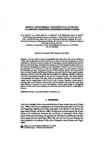
Fig. 1. Schematic diagram of the statistical model construction, a) unit volume of soil, b) the system of spheres that form overlapping layers, c) parallel connection of resistors in the layers and series between layers.

In our study we used the statistical-physical model of soil thermal conductivity [390]. This model is based on the terms of heat resistance (Ohm’s law and Fourier’s law), two laws of Kirchhoff and polynomial distribution [88]. The volumetric unit of soil in the model (Fig. 1a) consists of solid particles, water and air, is treated as a system made up of the elementary geometric figures, in this case spheres, that form overlapping layers (Fig. 1b). It is assumed that connections between layers of the spheres and the layer between neighbouring spheres will be represented by the serial and parallel connections of thermal resistors, respectively (Fig. 1c). Comparison of resultant resistance of the system, with consideration of all possible configurations of particle connections together with the mean thermal resistance of given unit volume of soil, allows the estimation of thermal conductivity of soil λ (W m–1 K – 1 ) according to the equation [390]: 4π (52) λ= L P ( x1 j ,..., x kj ) u∑ j =1 x1 j λ 1 (T )r1 + ... + x kj λ k (T )rk where: u is the number of parallel connections of soil particles treated as thermal resistors, L is the number of all possible combinations of particle configuration, x1, x2 ,..., xk – the number of particles of individual particles of a soil with thermal conductivity λ1, λ2 ,..., λk and particle radii r1, r2 ,..., rk, where

k

∑x i =1

ij

=u,

j=1,2,...,L, P(xij) – probability of occurrence of a given soil particle configuration calculated from the polynomial distribution:

24

u! x x f 1 1 j ... f k kj . ! x ...x kj

P( x1 j ,..., x kj ) =

! 1j

∑ P(X = x )= 1

(53)

L

The condition:

j

j =1

must also be fulfilled. The probability of

selecting a given soil constituent (particle) fi, i = s, c, g, in a single trial was determined based on fundamental physical soil properties. In this case f s , f c , and f g are the content of individual minerals and organic matter – f s = 1 − φ , liquid – f c = θ v and air – f g = φ − θ v in a unit of volume, φ – soil porosity. So far, investigations showed that to calculate soil thermal conductivity the conductivities of main soil components can be used [390]. They are: quartz, other minerals, organic matter, water and air. Their values of thermal conductivity and relations to temperature are presented in Table 1. Table 1. Values and expressions for parameters used in calculating the thermal conductivity of soils (T in oC).

Source a

Parameters b Expression, value b (W m-1 K-1) 9.103 - 0.028 T λq, 2.93 2 λmi, 2 0.251 λo, 1 0.552 + 2.34⋅10-3 T - 1.1⋅10-5 T2 λw, 1 0.0237 + 0.000064 T λa, a b 1. [162]; 2. [78], thermal conductivity of: quartz λq, other minerals, λmi, organic matter, λo water or solution, λw air, λa. Parameters of the model were defined earlier on the basis of empirical data [390,391]. The agreement between predicted and measured results was determined with a mean square error (σb) and relative maximum error (ηb): n

σb =

∑( f i =1

mi

− f ci )

k

2

,

(54)

where: fmi is the measured value, fci is the calculated value, k = n - 1 if n < 30 and k = n n > 30, n – number of data.

25

The relative maximum error was calculated using the following equation:

 f mi − f ci  ⋅ 100% .  f mi 

η b = max  i =1, 2 ,L, n

(55)

Also regression equations of the thermal conductivity and determination coefficient R2 were developed. Predicted thermal conductivity values were compared with measured data on the Fairbanks sand, Healy clay, Felin silty loam, Fairbanks peat and loam [78,390,391]. Regression coefficients were close to unity, however permanent factors in the equation were close to zero. Determination coefficients of the linear regression were high and ranged from 0.948 to 0.994. Mean square errors σ (W m–1 K–1) and relative maximum errors η(%) ranged from 0.057 to 0.123 (W m–1 K–1) and from 12 to 38.3%. These data indicate good performance of the model in predicting the thermal conductivity. Volumetric heat capacity Cv (MJ m–3 K–1) was calculated using empirical formulae proposed by de Vries [78]:

C v = (2.0 x s + 2.51x o + 4.19 x w ) ⋅ 10 6

(56)

where: xs , xo , xw (m3 m–3) – are volumetric contributions of mineral and organic components and water, respectively. Thermal diffusivity α was calculated from the quotient of the thermal conductivity and volumetric heat capacity:

α=

λ

Cv

.

(57)

4. TEMPORAL VARIATIONS IN THE AGRO-METEOROLOGICAL DATA

In this chapter we present some preliminary results for the analysis of temporal variations of agro-meteorological data. The novelty of our approach consists in the utilization of the following modern methods: • Wavelet transform (WT) • Empirical Mode Decomposition (EMD) • Multitaper Method (MTM)

26

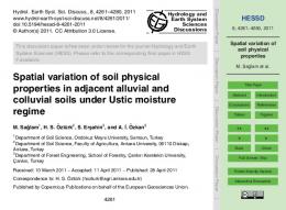
4.1.The data The analyzed data were recorded by the automatic agro-meteostation manufactured by Eijkelkamp Company (http://www.eijkelkamp.com/). The station is shown in Fig. 2.

Fig. 2. The automatic agro-meteostation of the type 16.98.

The following parameters are measured by the station: wind speed and wind direction, global radiation, air temperature, air humidity, soil temperature and precipitation. The wind data were not used in our analysis. The radiation sensor operates in a measuring range of 305-2800 nm with accuracy of 2.5%. The air temperature and relative humidity sensor with radiation shield measures temperature between –40°C and +60°C with accuracy of +/- 0.2°C, humidity between 0 to 100 % with accuracy better than 2%. The soil temperature sensor operates in a measuring range of –40°C and +60°C, accuracy 0.1°C at 0-50°C and 0.2°C at –40°C till +60°C. The last one, the rain gauge of UV-resistant plastic, aerodynamic design, and with a tipping bucket has a resolution of 0.2 mm precipitation and a surface area of 507 cm2.

27

The data covering the period of May-June 2003 are shown in Fig.3. Here we focus ourselves on the variation of soil temperature since it influences strongly crop development and plant growth. It is well known that soil temperature depends on both the soil surface energy balance and on the thermal properties of the soil [37,79,89,160]. As it is seen in Fig. 3 the daily soil temperature variations follow closely the air temperature and solar radiation. However, the bad weather and heavy precipitations can destroy this synchrony and we observe the intermittent behavior in these parameters. Such an intermittency is the main obstacle in using classical methods for the analysis of that kind of data. In addition, seasonal variations in the data can not be extracted easily. These are perhaps more important than daily variations. Due to the above reasons we have to resort to the afore-mentioned more advanced methods of data analysis. Air temperature deg C

40 20 0 120

130

140

150 Soil temperature

160

170

180

130

140

150 Solar radiation

160

170

180

130

140

150 Humidity

160

170

180

130

140

150 Rain

160

170

180

130

140

150 Day of year

160

170

180

deg C

40 20

kW/m2

0 120 1 0 -1 120

%

100 50 0 120

mm

10 5 0 120

Fig. 3. The data set recorded by the agro-meteostation during May-June 2003.

28

4.2.Wavelet transform Wavelet transform is a method that allows studying time series simultaneously at time-scale or equivalently in time-frequency domain. It means that WT due to its local nature is able to analyze properly any localized variations in the data. This aspect makes the WT very useful in the analysis of nonlinear and nonstationary time series. Most of the time or spatial series encountered in soil science belong to this category. Until now, the WT has not been widely used in the analysis of data in soil science. However, Lark with co-workers have shown in a series of papers that the WT should be considered as a standard tool in the analysis of various soil data. In a paper [187] the authors have shown how the wavelet transform can be used to analyze complex spatial variations of soil properties sampled regularly on transects. The paper can be treated as an introduction of wavelets to soil science. In another paper [192] they have studied variation and covariation in small data sets from soil survey. The data sets comprise measurements of pH and the contents of clay and calcium carbonate on a 3-km transect in Central England. In that paper they have used a variant of the WT, called the maximal overlap discrete wavelet transform (MODWT) developed in statistical community. Electrical conductivity of soil was analyzed using wavelets in a third paper [194]. Recently Lark’s group has widely studied an intermittent variation of nitrous oxide emissions from soils using wavelets [195,196,197,454]. In their most recent [198] the authors have successfully extended wavelet analysis to two dimensions. Every soil scientist seriously interested in using wavelets for the analysis of soil data should consult their paper. First we study the temporal variations in the data using Continuous Wavelet Transform (CWT). One of the most popular approaches in practice is the CWT based on the Morlet mother wavelet [374]. The popularity of this approach comes from the conceptual similarities to the Fourier orthogonal analyzing functions e-iωt. The Morlet wavelet (Fig. 4) is defined as follows:

ψ 0 (η ) = π −1 / 4 e iω η e −η 0

2

/2

,

(58)

where ω0 is dimensionless frequency and η is dimensionless time. To achieve the optimal localization in time and frequency usually ω0=6 is usually adopted. This choice also satisfies the admissibility condition. The Gaussian envelope exp(-η2/2) localizes the wavelet in time. Fourier frequency f and wavelet scale s

29

are not directly related. One has to rescale the result of wavelet analysis with a factor depending on the mother wavelet. For the Morlet wavelet, the conversion formula has the form:

1/ f =

4πs

ω0 + 2 + ω02

.

(59)

For ω0=6, s⋅f is approximately one. 0.8 0.6 0.4

Amplitude

0.2 0 -0.2 -0.4 -0.6 -0.8 -4

-3

-2

-1

0 Time

1

2

3

4

Fig. 4. The Morlet wavelet for ω0=6. Real part (solid line), imaginary part (dashed line).

The CWT of time series (xn, n=1,…,N) sampled uniformly with step dt is defined as the convolution of xn with the scaled and normalized wavelet and is given by:

WnX ( s ) =

dt dt N x n'ψ [(n ' − n) ]. ∑ s s n ' =1

(60)

30

Since the above equation is a convolution its computation can be efficiently implemented in the frequency domain by using the FFT algorithm. The details are omitted here but they can be found in the cited literature [195,196,197,454]. The 2

wavelet power is defined as WnX (s ) . The complex argument of WnX (s ) can be interpreted as the local phase. The CWT has edge artifacts because the Morlet wavelet is not completely localized in time. These are taken into account by introducing the Cone of Influence (COI). The COI is the area in which the wavelet power caused by a discontinuity at the edge drops to e-2 of the value at the edge. The cross wavelet transform (XWT) of two time series xn and yn is defined as:

W XY = W X W Y * ,

(61)

where: * denotes complex conjugation. Next, we define the cross wavelet power as W XY . Cross wavelet power reveals areas in the time-frequency plane with high common power. The complex argument arg( W XY ) can be interpreted as the local relative phase between xn and yn time series. We are often interested in the phase relationship between two time series. Following Torrence and Webster [375] we define the wavelet coherence of xn and yn time series as:

Rn2 ( s ) =

S ( s −1WnXY ( s )

2

2

2

S ( s −1 WnX ( s ) ) ⋅ S ( s −1 WnY ( s ) )

,

(62)

where: S is a smoothing operator. The wavelet coherence can be interpreted as a localized correlation coefficient in the time-frequency plane. The smoothing operator S has a form:

S (W ) = S scale ( S time (Wn ( s ))),

(63)

where: Sscale denotes smoothing along the wavelet scale axis and Stime smoothing in time. A suitable smoothing operator is given by Torrence and Webster [375]:

S scale (W ) s = (Wn ( s) ∗ c1e

−t

2

2s2

)s

(64)

31

S time (W ) n = (Wn ( s ) ∗ c 2 Π (0.6 s )) n ,

(65)

where: c1 and c2 are normalization factors and Π is the boxcar function. The value of 0.6 is the optimal for the Morlet wavelet. The wavelet coherence phase difference is given by the following equation:

 Im(S ( s −1WnXY ( s )))   XY −1 S s W s Re( ( ( ))) n  

φ n ( s) = tan −1 

(66)

The statistical significance of wavelet power can be estimated by comparison with the power spectrum of a first order autoregressive AR(1) process. This approach is based on the findings that many geophysical time series show red noise characteristics. The power spectrum of an AR(1) process is given by:

Pk =

1−α 2 1 − αe −i 2πk

2

,

(67)

where: k is the Fourier frequency index and α autocorrelation at lag equal to 1. Torrence and Compo [374] showed that for a given background spectrum Pk, the corresponding wavelet power at each time n and scale s is distributed as:

D(

WnX ( s )

σ

2 X

2

< p) =

1 Pk χ υ2 ( p), 2

(68)

where: ν is equal to 1 for real and 2 for complex wavelets, p is the desired significance (p = 0.05 for the 95 % confidence interval). Similarly, Torrence and Compo [374] have developed a formula for the joint distribution of the cross wavelet power to two time series with background power spectra PkX and PkY . It is expressed here as a:

D(

WnX ( s )WnY * ( s )

σ Xσ Y

< p) =

Zυ ( p)

υ

PkX PkY ,

(69)

where: Zν(p) is the confidence level associated with the probability p for the resulting probability density function defined as a square root of the product of two chi-square distributions. For ν = 2, Z2(95%) = 3.999.

32

The wavelet and cross-wavelet transform were computed with the package available at http://www.pol.ac.uk/home/research/waveletcoherence/. 4.3.The results of wavelet transform Fig. 5 show the CWT of the air temperature. The daily component is clearly seen. However, the seasonal component with a period greater than 128 hours for hours between 200 and 800 in the figure is much stronger. One can also notice the weak high-frequency component with the period of 8 hours. Fig. 6 show the CWT of the topsoil temperature. The similarities with the previous figure are obvious. One can note the reduced dynamics in the topsoil temperature variations. Both daily and seasonal components are of the comparable strength. High frequency variations are now shifted to the band around 12 hours. Fig. 7 shows the CWT of the solar radiation. Obviously, the daily component is strongest one. The seasonal component is the much weaker. One can also see a few little spots of the power along time in the band for 12 hours. In general, the daily course of the topsoil temperature follows closely the solar radiation for a given time. Fig. 8 show the CWT of the air humidity. The power variations with time for daily components are visible. Also long-term features are noticeable. The cross wavelet transform of the solar radiation and air temperature is shown in Fig. 9. The 5% significance level is shown as a thick contour. The arrows indicate the phase relationship between both time series. The time series are in-phase for arrows pointing right, anti-phase pointing left. As it is seen the air temperature is shifted in phase about 45° as compared to the solar radiation. In addition, this shift is noticeably greater for seasonal components. Fig. 10 show the cross wavelet transform of the solar radiation and topsoil temperature. Accordingly, the phase shift is now about 60°. The above results agree qualitatively with the theory of heat transfer, since the air and soil respond with the delay to driving force, i.e., the solar radiation. Fig. 11 show the cross wavelet transform of the solar radiation and air humidity. Comparing figures 9 and 11 one can conclude that the air temperature and humidity are in anti-phase. Moreover, the air humidity advances the solar radiation. According to the adopted convention, the phase shift is about –45°. Finally, Fig. 12 show the squared wavelet coherence between the solar radiation and air temperature. Again, the 5% significance level is shown as a thick contour. The coherence and constant phase relationship for daily and seasonal components are significant. We conclude that the cross wavelet analysis and wavelet coherence are powerful methods for testing causal relationship between two time series.

33

Fig. 5. The wavelet transform of the air temperature.

Fig. 6. The wavelet transform of the topsoil temperature.

34

Fig. 7. The wavelet transform of the solar radiation.

Fig. 8. The wavelet transform of the air humidity.

35

Fig. 9. Cross wavelet transform of the solar radiation and air temperature.

Fig. 10. Cross wavelet transform of the solar radiation and soil temperature.

36

Fig. 11. Cross wavelet transform of the solar radiation and humidity.

Fig. 12. Squared wavelet coherence between the standardized solar radiation and air temperature.

37

4.4.Empirical Mode Decomposition Empirical Mode Decomposition (EMD) has been pioneered by Huang et al. [148,149] for analysis of nonlinear and non-stationary time series. It has gained a lot of popularity in data analysis and is widely considered as a major breakthrough in applied mathematics in the 20th century. This technique adaptively decomposes the given oscillatory signal into a few AM-FM components which are referred to as Intrinsic Mode Functions (IMFs). IMFs are calculated in an iterative procedure called sifting process. As a rule, the last IMF represents long-term trend in the data. It is worth to note that this is local and fully data-driven technique. The EMD is in fact a type of adaptive wavelet decomposition whose subbands are built up in accordance with the frequency content of the signal. The original signal can be reconstructed by summing up all IMFs. However, we are often more interested in partial reconstructions. In other words, we want to analyze various components of the given signal separately. For example, one usually needs to detrend the data or to perform some kind of filtering. One should note that this can be realized completely easily with the IMFs. Estimation of the trend in data or band-pass filtering is equivalent to summing up suitably chosen the mutually orthogonal pairs of IMFs. The above approach is adopted in the present analysis of soil temperature and humidity data. The time-frequency spectrum, a post-processing aspect of EMD, which is estimated with Hilbert transform, will not be considered here. The EMD assumes that IMFs should: (1) have the same number of zero crossings and extrema; (2) be symmetric with respect to the local mean Given a signal x(t), the EMD algorithm works as follows: (1) find all the extrema of x(t); (2) connect all the local maxima by a cubic spline as an upper envelope emax(t); repeat the procedure for the local minima to obtain the lower envelope emin(t); (3) compute the average m(t) = (emin(t) +emax(t))/2; (4) extract the detail d(t) = x(t) - m(t); (5) iterate on the residual m(t). In practice, the above main loop is refined by a sifting process, an inner loop that iterates step (1) to (4) upon the detail signal d(t), until this latter can be considered as zero-mean according to some stopping criterion. Once this is achieved, the detail is considered as the effective IMF, the corresponding residual is computed and only then algorithm goes to step (5).

38

In summary, the original signal x(t) is first decomposed through the main loop as

x(t ) = d1 (t ) + m1 (t ),

(70)

and the first residual m1(t) is itself decomposed as

m1 (t ) = d 2 (t ) + m2 (t ),

(71)

so that

x(t ) = d 1 (t ) + m1 (t ) = d1 (t ) + d 2 (t ) + m2 (t ) = ... =

(72)

K

∑d k =1

k

(t ) + m K (t )

Although the EMD principle is very simple and appealing and its implementation easy, the exact mathematical theory of this method is not available yet. Due to the lack of analytical formulas its performance analysis is difficult. In spite of that, the EMD is widely used in different branches of science as a one of the best methods for the analysis of non-stationary time series. The reconstruction of signal components is done in a process of visual inspection and selection of the appropriate IMFs. Although the selection criterion is a bit arbitrary, one can readily identify particular IMSs which correspond to a given sub-band. Finally, the signal components are restored by summing up the carefully selected IMFs. Let us emphasize that the above very simple procedure is equivalent to the adaptive sub-band filtering. We illustrate how the EMD works using the same data we have analyzed with the CWT. 4.5.The results of EMD Fig. 13 show the EMD of the air temperature. As can be seen, the original time series is decomposed into eight IMFs. The reconstructed components, highfrequency variations (C1), periodic (daily) variations (sum of C2 to C4) and longterm (seasonal) variations (sum of C5 to C8) are shown in Fig. 14. The seasonal component is superimposed on the original time series, while the remaining

39

components are shown below in the figure. This same convention is used in subsequent figures. Note that the mean value of these two components is relative and equal to zero. Fig. 15 show the EMD of the topsoil temperature. In this case the high-frequency variations are not present. Of course, this is caused by greater thermal inertia of the soil as compared to the air. Fig. 16 show the two reconstructed components. The daily component comprises of C1 and C2 IMFs while the seasonal component the remaining IMFs (sum of C3 to C6). Fig. 18 shows the EMD of the air humidity. In this case, one can observe readily an increase of the air humidity caused by the precipitation. Fig. 19 show the three reconstructed components of the air humidity. The high-frequency component comprises of C1 IMF, the daily component (sum of C2 to C4), the seasonal (sum of C5 to C8). Note that the daily component is additionally shifted to the level – 50 % for presentation clarity. Finally, the EMD of the solar radiation is shown in Fig. 20 and the reconstructed components in Fig. 21. The visible valleys in the course of solar radiation are caused by the weather breakings. This intermittent behavior is instantly reflected in other measured quantities. The EMD of the solar radiation contains of nine IMFs. The high-frequency component comprises of C1 IMF, the daily component (sum of C2 to C4), the seasonal component (sum of C5 to C9). The daily component is additionally shifted to the level -1.5 kW/m2 for presentation clarity. The heat transfer regime at the air-soil interface can be studied with details by using the Empirical Mode Decomposition as demonstrated above. Two main factors play a major role here - solar radiation and intermittency in the weather. The dynamics of the air and topsoil temperature variations can be represented on the so-called phase-space plots. Fig. 17 shows such a plot for the daily and seasonal reconstructed components. As can be seen the dynamical picture of both variatiations is rather complex. It is worth to note that such representation is very useful in qualitative assessment of the heat transfer regime at the air-soil interface.

40

C8

C7

C6

C5

C4

C3

C2

C1

deg C

Air temperature 40 20 0 120 5 0 -5 120 10 0 -10 120 10 0 -10 120 5 0 -5 120 5 0 -5 120 5 0 -5 120 5 0 -5 120 18

130

140

150

160

170

180

130

140

150

160

170

180

130

140

150

160

170

180

130

140

150

160

170

180

130

140

150

160

170

180

130

140

150

160

170

180

130

140

150

160

170

180

130

140

150

160

170

180

130

140

150 Day of year

160

170

180

16 14 120

Fig. 13. The Empirical Mode Decomposition of the air temperature.

41

Reconstructed air temperature 35

30

25

20

deg C

15

10

5

0

-5

-10 120

130

140

150 Day of year

160

Fig. 14. The reconstructed three components of the air temperature.

170

180

42

Soil temperature deg C

40 20

C1

0 120 10

130

140

150

160

170

180

130

140

150

160

170

180

130

140

150

160

170

180

130

140

150

160

170

180

130

140

150

160

170

180

-2 120 50

130

140

150

160

170

180

0 120

130

140

150 Day of year

160

170

180

0

C2

-10 120 5 0

C3

-5 120 2 0

C4

-2 120 5 0

0

C6

C5

-5 120 2

Fig. 15. The Empirical Mode Decomposition of the topsoil temperature.

43

Reconstructed soil temperature 30

25

20

deg C

15

10

5

0

-5

-10 120

130

140

150 Day of year

160

Fig. 16. The reconstructed two components of the topsoil temperature.

170

180

44

Dynamics of the daily components

a) 180

Day of year

170 160 150 140 130 120 20 10

10

5 0

0 -5 -10

Air temperature (degC)

-10

Topsoil temperature (degC)

Dynamics of the seasonal components

b) 180

Day of year

170 160 150 140 130 120 25 20

25 15

20 10

Air temperature (degC)

15 5

10

Topsoil temperature (degC)

Fig. 17. Phase space plot of the air and topsoil temperature, (a) reconstructed daily components, (b) reconstructed seasonal components.

45

Humidity %

100 50

C1

0 120 10

C2 C3 C4

170

180

130

140

150

160

170

180

130

140

150

160

170

180

130

140

150

160

170

180

130

140

150

160

170

180

130

140

150

160

170

180

130

140

150

160

170

180

130

140

150

160

170

180

130

140

150 Day of year

160

170

180

0 -20 120 20

C5

160

0 -50 120 20

0 -20 120 10

C6

150

0 -50 120 50

0 -10 120 20

C7

140

0 -10 120 50

0 -20 120 65

C8

130

60 55 120

Fig. 18. The Empirical Mode Decomposition of the air humidity.

46

Reconstructed humidity 100

80

60

40

%

20

0

-20

-40

-60

-80

-100 120

130

140

150 Day of year

160

Fig. 19. The reconstructed three components of the air humidity.

170

180

47

C1

kW/m2

Solar Radiation 1 0 -1 120 0.5

C2 C3 C4 C5

170

180

130

140

150

160

170

180

130

140

150

160

170

180

130

140

150

160

170

180

130

140

150

160

170

180

130

140

150

160

170

180

130

140

150

160

170

180

130

140

150

160

170

180

130

140

150

160

170

180

130

140

150 Day of year

160

170

180

0 -0.2 120 0.2 0 -0.2 120 0.1

C6

160

0 -0.5 120 0.2

0 -0.1 120 0.1

C7

150

0 -1 120 0.5

0 -0.1 120 0.1

C8

140

0 -0.5 120 1

0 -0.1 120 0.35

C9

130

0.3 0.25 120

Fig. 20. The Empirical Mode Decomposition of the solar radiation.

48

Reconstructed Solar Radiation 1

0.5

kW/m2

0

-0.5

-1

-1.5

-2 120

130

140

150 Day of year

160

Fig. 21. The reconstructed three components of the solar radiation.

170

180

49

4.6.The Multitaper Method Usually, the power spectrum of a time series is estimated as the squared absolute value of its Fourier Transform. This simple approximation is called the periodogram. To reduce leakage in the spectral estimation, a time series is often windowed before applying the Fourier Transform. Although windowing reduces the bias, it does not reduce the variance of the spectral estimate. The multitaper method [290,371] is designed to reduce spectral leakage. First the dates are windowed with different, orthogonal tapers, and next spectra for all the tapers are averaged. The resulting multitaper spectral estimator is superior to the periodogram in terms of reduced bias and variance. There are some similarities with the Welch method of modified periodogram. The multitaper spectrum estimator is given by:

S( f ) =

1 L −1 ∑α k S k ( f ) L k =0

(73)

with

Sk ( f ) =

N −1

2

∑ wk (n) x(n)e − j 2πfn

(74)

n =0

where: αk is the corresponding weighting factor, N is the data length and wk(n) is the k-th data taper used for the spectral estimate Sk(f), which is also called k-th eigenspectrum. The tapers are orthonormal, i.e.,

∑

n

w k (n) w j (n) = 0 for j≠ k

and equal to 1 for j = k. The discrete prolate spheroidal sequences (dpss) or Slepian sequences are usually chosen as tapers because of their good leakage properties. The number of tapers L is always chosen to be less than 2NW, where W is expressed in units of normalized frequency, i.e., 0 < W < ½. The Slepian sequences maximize the spectral concentration of the window main lobe within [-W,W]. The multitaper cross spectral transform for time series xn and yn is given as

S

XY

1 L −1 X ( f ) = ∑ Fk ( f ) FkY ∗ ( f ), L k =0

(75)

50

where: N −1

FkX ( f ) = ∑ wk (n) x(n)e − j 2πfn ,

(76)

n=0

and similarly for yn. The multitaper coherence is defined here as:

C

XY

(f)=

S XY

,

(77)

Im(C XY ) ), Re(C XY )

(78)

SX

SY

and phase difference is given by:

φ = arctan(

We have used the improved matlab scripts for the computation of both the multitaper spectrum and coherence. These scripts were delivered by Peter Huybers and are available in the Matlab Central archive or in his home page http://web.mit.edu/~phuybers/www/Mfiles/index.html. It is worthwhile to note that these scripts use a fast approximation to compute the 95% confidence limits for a chi-squared distribution and computes the equivalent degrees of freedom as given by Percival and Walden, 1993, p256 and p370 [290]. Also the adaptive weights αk is determined iteratively (see above, pp.368-370). 4.7.The results of the Multitaper Method We have shown that the adaptive sub-band filtering of a given time series can be implemented readily with the EMD. How efficient is this technique? We answer this question by comparing the MTM power spectra of both the original time series and the reconstructed components. Fig. 22 shows the power spectrum of the air temperature. The background spectrum really resembles the red noise, since the power increases at low frequencies. There are apparent three distinct peaks in the spectrum. The strongest peak corresponds to the diurnal cycle; the next ones have periods of 12 and 8 hours. The high-frequency noise is also apparent. Fig. 23 shows the reconstructed daily components of the air and topsoil temperature. These components are quite similar. However, one can also notice minor differences in their course.

51

4

power density (units 2/cycle/deltat)

10

2

10

0

10

-2

10

-3

10

-2

10 frequency (cycles/deltat)

-1

10

Fig. 22. The multitaper power spectrum density of the air temperature.

Fig. 24 shows the MTM spectrum of the daily component of the air temperature. It is evident that low- and high-frequency power is diminished. Fig. 25 shows the high-frequency component of the air-temperature. The MTM power spectrum of this noisy component is shown in Fig. 26. Obviously, this confirms again that the EMD is highly efficient when one tries to filter out or isolate signal components. Fig.27 shows the coherence and phase difference for the daily components of the air and topsoil temperature. We draw our attention to the following frequencies, 0.04, 0.08 and 0.12 (cycles/delta t). Almost perfect coherence is seen for the main variation, still high for variation at frequencies 0.08 and 0.12. Notice also the progressive phase difference at these frequencies. Fig. 28 shows the seasonal components of the air and topsoil temperature. These are also quite similar. It is also apparent that the soil accumulates the thermal energy especially for days 145 to 175. Fig. 29 shows the coherence and the phase difference for the seasonal components. The coherence is also high and phase difference is increasing with the frequency. The above results agree well

52

with the wavelet analysis. However, we should emphasize here that the combined EMD-MTM analysis enables much deeper insight into the thermal regime at the air-soil interface.

Air temperature 15

deg C

10 5 0 -5 -10 120

130

140

150

160

170

180

160

170

180

Soil temperature 10

deg C

5 0 -5 -10 120

130

140

150 Day of year

Fig. 23. The reconstructed daily components of the air and topsoil temperature.

53

2

power density (units 2/cycle/deltat)

10

0

10

-2

10

-4

10

-6

10

-3

-2

10

10 frequency (cycles/deltat)

-1

10

Fig. 24. The multitaper power spectrrum density of the daily component of air temperature.

3

deg C

2 1 0 -1 -2 120

130

140

150 Day of year

160

Fig. 25. The high-frequency (noisy) component of the air temperature.

170

180

power density (units 2/cycle/deltat)

54

0

10

-1

10

-3

-2

10

10 frequency (cycles/deltat)

-1

10

Fig. 26. The multitaper power spectrum density of the noisy component of air temperature. mean is 0.31 32% of estimates above 95% confidence level

coherence

1

0.5

0 0.02

0.04

0.06

0.08 frequency

0.1

0.12

0.14

0.04

0.06

0.08 frequency

0.1

0.12

0.14

0

phase

-50

-100

-150 0.02

Fig. 27. The multitaper coherence and phase difference for daily components of air and topsoil temperature.

55 25

deg C

20 15

Topsoil Air

10 5 120

130

140

150 Day of year

160

170

180

Fig. 28. The reconstructed seasonal components of the air and topsoil temperature. mean is 0.34 36% of estimates above 95% confidence level

coherence

1

0.5

0

0.002 0.004 0.006

0.008

0.01 0.012 0.014 0.016 0.018 frequency

0.02

0.002 0.004 0.006

0.008

0.01 0.012 0.014 0.016 0.018 frequency

0.02

30 20 phase

10 0 -10 -20 -30

Fig. 29. The multitaper coherence and phase difference for the seasonal components of air and topsoil temperature.

56

5. STATISTICAL AND GEOSTATISTICAL ANALYSES OF TIME SERIES OF THE PHYSICAL VALUES AND PROPERTIES OF SOIL 5.1. Field experiment The data analyzed in this monograph originated from two sources. The first was the measurement data acquired within the research project „Structure of radiation balance and the thermal-moisture relations of soil”, Grant KBN, No. PB 1679/5/91 headed by Prof. R.T. Walczak [416]. The second – data collected within the research project KBN No. 6 P06H 029 20 (2001-2003) „Investigation of spatial variability of physicochemical soil properties as a base for precision agriculture„ State Committee for Scientific Research, during the period of 20012003, headed by the first of the authors of this monograph. In the case of the first object of investigation, measurements were taken in an experimental plot of the Agrometeorological Station, University of Agriculture, Lublin, in the field of the Agricultural Experimental Station, University of Agriculture, located next to the Institute of Agrophysics in Lublin (Felin, 51°13'29" N 22°38'42" E). The soil at Felin is classified as a grey brown podzolic soil. R. Turski (verbal information) classified the soil at Felin as a grey brown podzolic soil developed from a loess-like formation, incomplete, on a chalk formation. In the object studied, the following soil profile was determined: from 0 to about 20 cm – humus horizon with brown-grey colouring, distinctly separated from the next layer with reddish colouring, below 30 cm somewhat lighter in colour with yellow spots and with high sand content. From the depth of about 45 dm there appear fragments of weathered lime rock which becomes a significant material component of the soil below 90 cm [169]. The Table 2 presents the granulometric composition and some physical-chemical properties of the soil at the Agricultural Experimental Station, University of Agriculture (further referred to as the RZD AR Station) at Felin near Lublin [207]. The measurements were taken on the object with plant canopy and without plants (as reference). The measurements were taken within the period of AprilJuly, 1993. The arrangement of the experimental plots, 50 x 40 m in size, was such that they were strung along a road passing through the middle of the station area. The fallow plot and the meteorological station plot had constant positions during the measurement seasons, while particular cultures were located on plots with an annual cycle of rotation (a specific culture would be moved in successive years by one plot in anticlockwise direction). TDR probes, spaced at 0.2 m from one another, were installed opposite the midpoints of the plots, in a row at the

57

distance of 3 m from the path. Each of the probes had one moisture sensor. The moisture sensors covered 5 cm soil layers and were installed in the plots in the soil layers of 0-0.05, 0.05-0.1, 0.1-0.15, 0.2-0.25, 0.3-0.35, 0.4-0.45, 0.5-0.55, 0.8-0.85 m. Measurements of soil moisture were taken once a day, in the afternoon hours. The time required to take measurements at all the measurement points in he experiment was approximately half an hour. Soil density was determined according to the gravimetric method, on the basis of soil cores sampled with cylinders 100 cm3 in volume and 5 cm high from the levels of TDR probe installation, down to the depth of 85 cm. The density measurements were taken in close proximity to the moisture sensors (about 0.5 m from the sensors) at the end of the moisture measurement sessions. Three soil cores were sampled from each horizon. The main mineral components of the soil, i.e. quartz and other minerals, were determined from the granulometric distribution assuming that the 1-0.02 mm fraction contains mainly quartz, and other minerals are contained in the fraction below 0.02 mm [78,390]. Table 2. Granulometric composition and some physical-chemical properties of the soil at the RZD AR Station, Felin near Lublin [207]. % content of granulometric fraction < 1 mm Layer (cm)

1-0.1

0.1

0.05

0.02

0.006

-0.05

-0.02

-0.006

-0.002

< 0.002

pH (KCl)

OM (%)

PD (Mgm-3)

0-15

20

6

42

23

3

6

5.8

1.48

2.61

30-40

16

10

42

13

6

13

5.4

-

2.63

80-90

66

10

9

4

3

8

5.6

-

2.58

OM – organic matter, PD – particle density of solid fraction.

5.2. Results of statistical analysis The distribution of atmospheric precipitation during the period of the study is presented in Fig. 30a. The sum of precipitation for that period was 167.5 mm in total; the maximum recorded precipitation occurred on the 174th day of the year and amounted to 27.9 mm. The effect of precipitation is most visibly reflected in the plot without plants, in the surface horizon of the soil (Fig. 31c), while the presence of plant canopy has a distinctly damping effect on the temporal runs of soil moisture. The extent to which plants could change the time runs of soil moisture depended on their stage of development (i.e. the intensity of water

58

uptake by their roots), on the water interception on a given plant, and on the surface runoff which in turn was determined by the degree of compaction of the surface horizon of the soil (Fig. 30b). 30

a)

Rainfall (mm)

25 20 15 10 5 0 110

130

150 170 Day of year

190

210

-3

Bulk density (Mg m )

1.7

b)

1.6 1.5 1.4 1.3

Spring Barley Rye Bare soil

1.2 1.1 1 0

0.2

0.4

0.6

0.8

Depth (m) Fig. 30. Precipitation (a) as a function of time and soil bulk density (b) of spring barley, rye and bare soil.

The mean values of soil density measured in the plots are shown, with relation to depth, in Fig. 30b. The lowest density was observed in the field with barley, in the arable layer, and the highest in the field with rye. Below the arable layer, the differentiation of soil density in the objects studied was only slight. The soil density distributions observed in the particular plots were related primarily to the time that elapsed from the last tillage applied, to the meteorological conditions,

59

and to the occurrence of the same genetic horizons at different depths in particular cultivation plots. Water content (m3 m-3 )

0.4

a)

0.3 0.2 0.1 0 110

150 170 Day of year

190

210

130

150 170 Day of year

190

210

0.4 Water content (m3 m-3)

b)

130

0.3 0.2 0.1 0 110

c) Water content (m3 m-3 )

0.4 0.3 0.2 0.1

z=0 m z=0.2 m z=0.5 m

z=0.05 m z=0.3 m z=0.8 m

z=0.1 m z=0.4 m

0 110

130

150 170 Day of year

190

210

Fig. 31. Soil water content as a function of time for different depths (a - spring barley, b - rye, c bare soil) during growing season.

Thermal conductivity (W m-1K-1)

2.5 2 1.5 1 0.5 0 110

130

150 170 Day of year

190

110

130

150 170 Day of year

190

210

2.5 2 1.5 1 0.5 0 210

2.5

-1

c)

-1

b)

Thermal conductivity (W m K )

a)

Thermal conductivity (W m-1K-1 )

60

2 1.5 1 z=0 m z=0.2 m z=0.5 m

0.5

z=0.05 m z=0.3 m z=0.8 m

z=0.1 m z=0.4 m

0 110

130

150 170 Day of year

190

210

Rys. 32. Soil thermal conductivity as a function of time for different depths (a - spring barley, b rye, c - bare soil) during growing season.

61

3.0E+06 Heat capacity (J m-3 K-1 )

a)

2.5E+06 2.0E+06 1.5E+06 1.0E+06 110

130

150

170

190

210

190

210

Day of year

b) Heat capacity (J m-3 K-1)

3.0E+06 2.5E+06 2.0E+06 1.5E+06 1.0E+06 110

c)

130

150 170 Day of year

-3

-1

Heat capacity (J m K )

3.0E+06 2.5E+06 2.0E+06 1.5E+06 z=0 m z=0.2 m z=0.5 m

1.0E+06 110

130

z=0.05 m z=0.3 m z=0.8 m

150 170 Day of year

z=0.1 m z=0.4 m

190

210

Rys. 33. Soil heat capacity as a function of time for different depths (a - spring barley, b - rye, c bare soil) during growing season.

62

1.2E-06 Thermal diffusivity (m2 s-1 )

a)

1.0E-06 8.0E-07 6.0E-07 4.0E-07 2.0E-07 130

150 170 Day of year

190

210

130

150 170 Day of year

190

210

1.2E-06

-1 2

b)

Thermal diffusivity (m s )

110

1.0E-06 8.0E-07 6.0E-07 4.0E-07 2.0E-07 110

1.2E-06 2

-1

Thermal diffusivity (m s )

c)

1.0E-06 8.0E-07 6.0E-07 z=0 m z=0.1 m z=0.3 m z=0.5 m

4.0E-07

z=0.05 m z=0.2 m z=0.4 m z=0.8 m

2.0E-07 110

130

150 170 Day of year

190

210

Rys. 34. Soil thermal diffusivity as a function of time for different depths (a - spring barley, b - rye, c - bare soil) during growing season.

63 Table 3. Summary statistics for water content, thermal conductivity, heat capacity and thermal diffusivity of spring barley. Depth (m)

0

0.5

0.1

0.2

0.3

0.4

0.5

0.8

Whole profile

Water content (m3 m-3) Mean

0.195

0.21

0.219

0.199

0.258

0.229

0.232

0.214

0.219

Minimum

0.108

0.14

0.149

0.142

0.204

0.19

0.189

0.167

0.108

Maximum

0.343

0.325

0.31

0.272

0.318

0.278

0.278

0.249

0.343

Std.Dev.

0.054

0.049

0.047

0.043

0.036

0.031

0.033

0.027

0.045

Coef.Var(%)

27.8

23.1

21.4

21.7

13.9

13.7

14.4

12.5

20.5

Skewness

0.612

0.276

-0.009

0.305

0.283

0.211

0.150

-0.294

0.021

Kurtosis

2.969

1.823

1.798

1.685

1.435

1.310

1.208

1.441

2.362

-1

-1

Thermal conductivity (W m K ) Mean

0.771

1.185

1.086

1.340

2.111

1.840

1.603

1.995

1.491

Minimum

0.361

0.644

0.691

0.960

2.034

1.743

1.416

1.888

0.361

Maximum

1.355

1.583

1.404

1.626

2.191

1.942

1.721

2.070

2.191

Std.Dev.

0.268

0.250

0.242

0.225

0.052

0.081

0.089

0.066

0.479

Coef.Var(%)

34.8

21.1

22.3

16.8

2.5

4.4

5.6

3.3

32.1

Skewness

0.253

-0.273

-0.403

-0.216

0.030

0.038

0.119

-0.374

-0.401

Kurtosis

2.364

1.875

1.839

1.782

1.467

1.247

1.327

1.579

2.145

6

-3

-1

Heat capacity × 10 (J m K ) Mean

1.683

1.852

1.841

1.865

2.309

2.107

2.033

2.107

1.975

Minimum

1.318

1.559

1.550

1.629

2.083

1.943

1.852

1.912

1.318

Maximum

2.300

2.333

2.223

2.172

2.560

2.311

2.224

2.255

2.560

Std.Dev.

0.227

0.203

0.196

0.181

0.150

0.131

0.140

0.112

0.253

Coef.Var(%)

13.5

11.0

10.6

9.7

6.5

6.2

6.9

5.3

12.8

Skewness

0.612

0.276

-0.009

0.305

0.283

0.211

0.150

-0.295

-0.181

Kurtosis

2.968

1.824

1.798

1.685

1.436

1.311

1.208

1.442

2.546

Thermal diffusivity × 10-7 (m2 s-1) Mean

4.454

6.331

5.824

7.135

9.166

8.742

7.892

9.475

7.377

Minimum

2.738

4.129

4.455

5.892

8.561

8.404

7.649

7.177

2.738

Maximum

6.002

7.147

6.623

7.790

9.763

8.997

8.118

9.873

9.873

Std.Dev.

1.011

0.738

0.759

0.593

0.372

0.173

0.126

0.203

1.752

Coef.Var(%)

22.7

11.7

13.0

8.3

4.1

2.0

1.6

2.1

23.8

Skewness

-0.402

-1.043

-0.814

-0.960

-0.315

-0.274

0.035

0.274

-0.604

Kurtosis

2.118

3.472

2.215

2.855

1.435

1.643

1.635

1.447

2.578

64 Table 4. Summary statistics for water content, thermal conductivity, heat capacity and thermal diffusivity of rye. Depth (m)

0

0.5

0.1

0.2

0.3

0.4

0.5

0.8

Whole profile

Water content (m3 m-3) Mean

0.215

0.221

0.218

0.221

0.237

0.221

0.209

0.258

0.225

Minimum

0.135

0.156

0.163

0.188

0.190

0.187

0.171

0.236

0.135

Maximum

0.325

0.326

0.322

0.287

0.310

0.300

0.295

0.287

0.326

Std.Dev.

0.044

0.044

0.036

0.032

0.033

0.035

0.038

0.012

0.038

20.6

19.8

16.6

14.3

13.9

15.8

18.0

4.8

16.9

Coef.Var(%) Skewness

0.470

0.527

0.771

0.789

0.600

0.820

0.865

-0.026

0.292

Kurtosis

2.592

2.260

3.072

2.248

2.072

2.368

2.480

1.885

2.195

Thermal conductivity (W m-1 K-1) Mean

1.705

1.773

1.863

1.591

1.809

1.598

1.996

2.038

1.797

Minimum

1.368

1.479

1.676

1.423

1.694

1.432

1.914

2.004

1.368

Maximum

1.939

1.973

2.037

1.761

1.955

1.717

2.142

2.087

2.142

Std.Dev.

0.141

0.122

0.085

0.087

0.076

0.093

0.081

0.016

0.181

Coef.Var(%)

8.3

6.9

4.6

5.5

4.2

5.8

4.1

0.8

10.1

Skewness

-0.631

-0.470

-0.049

0.647

0.167

0.519

0.454

-0.321

-0.147

Kurtosis

2.983

2.681

2.445

2.039

1.783

2.085

1.674

4.228

2.041

Heat capacity × 106 (J m-3 K-1) Mean

2.018

2.059

2.077

1.990

2.121

1.992

2.096

2.275

2.078

Minimum

1.684

1.788

1.849

1.851

1.925

1.850

1.938

2.185

1.684

Maximum

2.479

2.499

2.513

2.264

2.427

2.323

2.456

2.398

2.513

Std.Dev.

0.185

0.183

0.151

0.132

0.138

0.146

0.157

0.521

0.171

9.2

8.9

7.3

6.7

6.5

7.3

7.5

2.3

8.2

Coef.Var(%) Skewness

0.470

0.529

0.771

0.789

0.601

0.821

0.866

-0.027

0.276

Kurtosis

2.594

2.265

3.070

2.247

2.074

2.369

2.481

1.884

2.054

Thermal diffusivity × 10-7 (m2 s-1) Mean

8.457

8.627

8.986

8.001

8.542

8.029

9.541

8.958

8.643

Minimum

7.823

7.898

8.107

7.691

8.055

7.652

8.721

8.702

7.652

Maximum

8.838

9.019

9.381

8.160

8.840

8.210

9.879

9.176

9.879

Std.Dev.

0.248

0.269

0.262

0.129

0.215

0.159

0.319

0.147

0.533

2.9

3.1

2.9

1.6

2.5

2.0

3.3

1.6

6.2

Skewness

-0.615

-0.686

-1.173

-0.839

-0.750

-0.816

-1.176

0.080

0.359

Kurtosis

2.516

2.677

4.236

2.324

2.507

2.411

3.206

1.434

2.477

Coef.Var(%)

65 Table 5. Summary statistics for water content, thermal conductivity, heat capacity and thermal diffusivity of bare soil. Whole Depth (m) 0 0.5 0.1 0.2 0.3 0.4 0.5 0.8 profile 3 -3 Water content (m m ) Mean

0.155

0.270

0.254

0.218

0.243

0.264

0.302

0.333

0.255

Minimum

0.111

0.239

0.219

0.197

0.212

0.247

0.289

0.322

0.111

Maximum

0.278

0.332

0.305

0.243

0.267

0.284

0.311

0.345

0.345

Std.Dev.

0.034

0.021

0.023

0.013

0.013

0.010

0.005

0.005

0.053

22.1

7.7

9.0

6.0

5.2

3.7

1.6

1.6

20.9

Skewness

1.056

0.243

0.189

0.309

0.071

0.332

-0.196

-0.081

-0.631

Kurtosis

3.870

2.415

1.833

1.973

2.299

2.026

2.384

2.481

3.207

Coef.Var(%)

Thermal conductivity (W m-1 K-1) Mean

0.821

1.867

1.817

1.706

2.032

2.095

2.062

2.132

1.816

Minimum

0.239

1.814

1.730

1.642

1.981

2.077

2.056

2.115

0.550

Maximum

0.406

1.954

1.900

1.776

2.059

2.127

2.066

2.162

2.162

Std.Dev.

0.254

0.037

0.045

0.050

0.024

0.017

0.002

0.007

0.413

Coef.Var(%)

30.9

2.0

2.5

2.9

1.2

0.8

0.1

0.3

22.7

Skewness

-1.056

-0.206

-0.084

0.170

-0.599

0.836

-0.168

1.315

-1.943

Kurtosis

3.870

1.840

1.957

1.440

2.025

2.214

2.131

12.955

5.834

Heat capacity × 106 (J m-3 K-1) Mean

1.621

2.254

2.177

2.019

2.221

2.322

2.445

2.589

2.206

Minimum

1.436

2.125

2.030

1.931

2.091

2.251

2.391

2.544

1.436

Maximum

2.134

2.513

2.390

2.124

2.321

2.405

2.483

2.641

2.641

Std.Dev.

0.143

0.872

0.955

0.549

0.524

0.410

0.204

0.220

0.284

8.8

3.9

4.4

2.7

2.4

1.8

0.8

0.9

12.9

Coef.Var(%) Skewness

1.057

0.243

0.194

0.306

0.066

0.334

-0.200

-0.088

-0.919

Kurtosis

3.869

2.411

1.832

1.973

2.307

2.029

2.385

2.600

3.510

-7

2 -1

Thermal diffusivity × 10 (m s ) Mean

4.977

8.292

8.351

8.446

9.148

9.022

8.432

8.235

8.113

Minimum

3.832

7.774

7.951

8.316

8.870

8.844

8.319

8.094

3.832

Maximum

6.993

8.537

8.653

8.603

9.472

9.228

8.597

8.401

9.472

Std.Dev.

1.091

0.164

0.174

0.071

0.124

0.093

0.061

0.061

1.291

Coef.Var(%)

21.9

2.0

2.1

0.8

1.4

1.0

0.7

0.7

15.9

Skewness

0.433

-0.507

-0.136

0.025

-0.405

0.202

0.235

0.189

-2.285

Kurtosis

1.597

2.647

2.138

2.351

2.908

2.106

2.423

2.900

7.361

66

The time runs of soil moisture, thermal conductivity, capacity and diffusivity in the plots with barley and rye and in the bare plot are presented in Fig. 31, 32, 33, 34. The dynamics of particular variables was related to the stage of plant development in the plots under study. Rye, which was already well grown and had time to consume most of the water available in the soil, caused a continual decrease in the soil moisture. In turn, the condition of the plants did not permit the soil to be re-supplied with water from precipitation, as only the surface horizon of the soil increased its moisture content slightly after a rainfall. Barley, which during the period of the experiment went through all of its development stages, shows in the soil moisture distribution both the amount of water used for plant growth and the amount of water that reached the soil surface. The bare field was characterized by the most uniform distribution of moisture in the soil profile. The surface horizon of the fallow plot was characterized by the strongest dynamics and effect of precipitation on soil moisture. The thermal properties of the soil (Fig. 32, 33, 34) reflected primarily the moisture status of the soil (Fig. 31), and to a lesser extent – the soil compaction condition (Fig. 30b). The time runs of the heat capacity of the soil conformed with the soil moisture runs. Slightly less similar to the moisture runs were the time runs of the thermal conductivity. In the case of the thermal diffusivity they were distinctly different from the moisture runs. In some of the diffusivity runs a certain reflection of the moisture runs could be noticed, but in most of them the diffusivity increased with a reduction in the soil moisture content (Fig 34). This type of time runs indicates that with a certain soil density the thermal diffusivity of the soil was already beyond its maximum, and a decrease in the soil moisture resulted in a diffusivity shift towards its maximum. The mean values of soil moisture within the whole profile were similar in the plots with plants, and somewhat different in the bare plot. The plots with plants had relatively uniform moisture distributions within the profile; the bare plot was characterized by a considerable drop in soil moisture values in the surface horizon, below which the values were more homogeneous. The mean values of soil density in the rye plot and in the fallow were almost the same; in the barley plot the mean soil density was lower than in the fallow. The mean values of the thermal properties in the soil profile did reflect the water content in the soil, but in the case of thermal conductivity and diffusivity the barley plot had values somewhat lower than the rye plot, even though the soil moisture of the barley plot was higher, but in this case the conductivity and diffusivity were also significantly affected by the soil density which was higher in

67

the rye plot. The heat capacity of the soil conformed to the soil moisture distribution in the plots. Standard deviation was used as a measure of the scatter of soil moisture values. The greatest scatter was observed in the plots with plant canopy, the smallest in the bare plot. Coefficients of variability calculated for the whole profile in particular plots were the highest for the moisture in the rye plot and for the thermal properties in the barley plot. The lowest variability was observed in the case of moisture in the bare plot and the thermal properties in the rye plot. Analyzing the soil profiles, the greatest variability was observed for the moisture and thermal properties in the barley plot, and the smallest variability within the profile for moisture, heat capacity, and thermal conductivity and diffusivity of soil for horizons below 0.1 m was observed in the bare plot. In the case of thermal conductivity and diffusivity of soil in the 0-0.1 m the lowest values were observed in the rye plot. Statistics characterizing the soil moisture distributions − histograms (asymmetry and kurtosis) indicate mainly a slight right-hand asymmetry and a somewhat smaller than normal distribution concentration of soil moisture values around its mean value (normal distribution - asymmetry equal 0, kurtosis equal 3). Distribution of the heat capacity of the soil were similar to those of soil moisture. Thermal conductivity and diffusivity of the soil showed a largely left-hand asymmetry in the distribution of values and somewhat smaller than normal distribution concentration of values of those thermal properties of the soil around their mean values. 5.3. Results of correlation analysis Calculations of linear correlation of the soil features under consideration were performed at the significance level of p 0.9, RSS