Spatial Distribution of Soil Properties in Water ... - CiteSeerX

Published online August 3, 2006

Spatial Distribution of Soil Properties in Water Conservation Area 3 of the Everglades Reproduced from Soil Science Society of America Journal. Published by Soil Science Society of America. All copyrights reserved.

Gregory L. Bruland, Sabine Grunwald,* Todd Z. Osborne, K. Ramesh Reddy, and Susan Newman levels of detail than ever before (Miller et al., 2004). These methods can be used to quantify anthropogenic impacts to wetlands at multiple scales, providing valuable information to aid in the design of wetland restoration projects. There are numerous landscapescale wetland restoration projects in various phases of planning and implementation that are designed to ameliorate the effects of hydrologic alteration and nutrient loading, including the Chesapeake Bay (Teal and Peterson, 2005), the Mississippi River basin (Mitsch et al., 2001), the Florida Everglades (Sklar et al., 2005), and the wetlands of Iraq (Richardson et al., 2005). This study presents the results of research conducted in the Florida Everglades to assess how the spatial distribution of soil properties have responded to anthropogenically induced changes to this ecosystem. Historically, the Everglades was characterized by its large spatial extent, its heterogeneous mosaic of Cladium jamaicense Crantz (sawgrass) marsh, wet sloughs and tree islands, and its hydrologic regime of slow-moving sheet flow with long periods of inundation (Parker, 1974; McCally, 1999). These conditions allowed for the development of a peat-based subtropical wetland that was oligotrophic (Davis and Ogden, 1994) and P limited (Koch and Reddy, 1992). Hydrologic modification, drainage, wetland conversion, landscape fragmentation, and nutrient enrichment have significantly affected the ecology of the Everglades (Davis and Ogden, 1994). Starting in the 1880s, the construction of a network of nearly 2400 km of canals and dikes served to drain and compartmentalize the Everglades landscape into multiple discontinuous hydrologic units, including the Everglades Agricultural Area (EAA), the Water Conservation Areas (WCA-1, 2A, 2B, 3A, and 3B), and the Everglades National Park (Noe et al., 2001) (Fig. 1). The WCAs, created during the 1950s, are used for water storage, flood control, wildlife habitat, and recreation. Water management has increased the frequency and intensity of floods, droughts, and fire in the WCAs (DeAngelis and White, 1994; Gunderson, 1994; Smith et al., 2001). The increase in canals and disturbed areas in the WCAs changed the natural hydroperiods of these wetlands, creating deeper water conditions in some areas and overdrainage in others (Walters et al., 1992; David, 1996). In addition to hydrologic alteration, agricultural activities to the north and urbanization to the east have increased nutrient loading, especially in the form of P to the Everglades wetlands (Noe et al., 2001). Changes in hydrology combined with increased nutrient loading have led to significant changes in ecosystem structure and function (Davis, 1991; Koch and

ABSTRACT The need to integrate environmental responses at the landscape scale is a reoccurring theme in biogeochemistry and ecology. This linkage can be addressed by using geostatistics to examine spatial patterns and then assessing the relationships of these patterns to known ecosystem drivers. In this study, we used a stratified random sampling design to collect soil cores from 388 sites to quantify the spatial distribution of soil properties in a 233 000 ha subtropical wetland, Water Conservation Area 3 (WCA-3). To reflect hydrologic boundaries within the system, WCA-3 was divided into three zones: 3AN, 3AS, and 3B. Interpolated maps indicated that the highest levels of bulk density were located in western 3AN, whereas the highest total phosphorus (TP) values were located in northern 3AN and in areas adjacent to a canal bisecting the area. Twenty-five percent of 3AN had TP concentrations in the 0- to 10-cm layer . 500 mg kg21, indicating enrichment beyond historic levels. Only 5% of 3AS and 6% of 3B showed TP . 500 mg kg21. Total nitrogen (TN) and carbon (TC) were lowest in western 3AN, whereas the rest of WCA-3 had higher and more homogenous TN and TC distributions. Overall, distributions of soil properties were more homogeneous in 3AS than they were in 3AN or 3B. The approach used in this study provides a model for assessing current impacts to WCA-3, supplies baseline conditions against which future restoration efforts can be evaluated, and could be used in other landscape-scale wetland restoration projects.

T

spatial distribution of soil properties across wetland landscapes represents the combined effects and interactions of various biotic and abiotic factors (Bruland and Richardson, 2004; Grunwald et al., 2006a). Consequently, existing landscape patterns contain information about the processes that generated these patterns (Holling and Gunderson, 2002). In various wetlands around the world, the processes of hydrologic modification and nutrient loading have affected not only the structure and function of these ecosystems but also their spatial extent and distribution (DeBusk et al., 1994; Newman et al., 1997; Bruland and Richardson, 2005; Richardson et al., 2005). The use of global positioning systems, geographic information systems, and geostatistics has enhanced scientists’ capacity to describe patterns in nature over larger spatial scales and at finer HE

G.L. Bruland, S. Grunwald, T.Z. Osborne, and K.R. Reddy, Univ. of Florida, Institute for Food and Agric. Sciences, Soil and Water Science Dep., 2169 McCarty Hall, P.O. Box 110290, Gainesville, FL 32611-0290; Gregory L. Bruland, Univ. of Hawai’i at Manoa, College of Tropical Agriculture and Human Resources, Dep. of Natural Resources and Environmental Management, 1910 East-West Rd., Honolulu, HI 96822; Susan Newman, Everglades Division, South Florida Water Management District, West Palm Beach, FL 334164680. Received 27 Apr. 2005. *Corresponding author (SGrunwald@ ifas.ufl.edu). Published in Soil Sci. Soc. Am. J. 70:1662–1676 (2006). Wetland Soils doi:10.2136/sssaj2005.0134 ª Soil Science Society of America 677 S. Segoe Rd., Madison, WI 53711 USA

Abbreviations: Db, bulk density; IDW, inverse distance weighting; TAl, total aluminum; TC, total carbon; TCa, total calcium; TFe, total iron; TMg, total magnesium; TN, total nitrogen; TP, total P; TPi, total inorganic P.

1662

Reproduced from Soil Science Society of America Journal. Published by Soil Science Society of America. All copyrights reserved.

BRULAND ET AL.: SPATIAL DISTRIBUTION OF SOIL PROPERTIES IN WCA3 OF THE EVERGLADES

1663

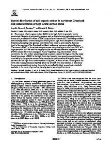
Fig. 1. Maps of (a) Florida and (b) South Florida with water flow direction (modified from Mitsch and Jørgensen [2004]) and (c) WCA-3 with the locations of the unit boundaries, canals, roads, water control structures, and 388 sites from the 2003–2004 sampling event.

Reddy, 1992; Drake et al., 1996, Newman et al., 1998; McCormick and Stevenson, 1998). Soils are an integrator of long-term environmental change (DeBusk et al., 1994; Craft and Richardson, 1997; Bruland et al., 2003; King et al., 2004). In the Everglades, soil chemistry has been shown to explain more variation in algal community attributes than water chemistry (Pan et al., 2000). Furthermore, nutrient inputs to Everglades wetlands are primarily stored in the peat, so

the vegetation represents only a short-term nutrient sink (Craft and Richardson, 1993a; Newman et al., 1997). Thus, the spatial distribution of soil nutrients can be used as a means of assessing long-term nutrient impacts to this system (Newman et al., 1997). Correspondingly, soils are an ideal ecosystem component for assessing the baseline status of WCA-3 before initiation of landscape-scale restoration activities. Because this area will be a central focus of future Comprehen-

Reproduced from Soil Science Society of America Journal. Published by Soil Science Society of America. All copyrights reserved.

1664

SOIL SCI. SOC. AM. J., VOL. 70, SEPTEMBER–OCTOBER 2006

sive Everglades Restoration Plan activities (U.S. Department of the Interior, 2005; U.S. Army Corps of Engineers, 2005), it is essential that the pre-restoration edaphic conditions of this ecosystem are quantified so that changes in soil properties caused by future management and restoration of WCA-3 can be assessed. Mapping the spatial distribution of soil properties across WCA-3 allows for the targeting and prioritization of areas for restoration and management and will facilitate the assessment of the future effects of restoration activities. The objectives of this study were to quantify spatial distributions of soil properties across three zones of Water Conservation Area 3 (3AN, 3AS, and 3B) (Fig. 1) and to compare and contrast these distributions among the floc, 0- to 10-cm, and 10- to 20-cm layers. MATERIALS AND METHODS Study Area WCA-3 is bounded to the north by the L-5 levee, the Rotenberger and Holeyland wildlife management areas, and the EAA (Fig. 1). It is bounded in the south by the L-29 levee and the Tamiami Trail. To the west lies the Big Cypress National Preserve, and to the east lies WCA-2A and 2B and the greater Miami metropolitan area. Of the WCAs, WCA-3 is the only area not entirely enclosed by levees. An 11-km stretch, called the L-28 Gap, has been left open on the western side to allow for overland flow between WCA-3 and the Big Cypress National Preserve. The surface hydrology of WCA-3 is controlled by a system of levees and water control structures located along the perimeter and inside the area. In 1962, WCA-3 was divided into two hydrologic units, WCA-3A and WCA-3B, by the construction of two interior levees (L-67A and L-67C) to reduce water losses due to levee seepage (Reddy et al., 1998). Interstate 75 (Alligator Alley) bisects WCA-3A in an east-west direction, further dividing WCA-3A into two zones, 3AN (the area to the north of Interstate 75) and 3AS (the area south of I-75) (Fig. 1). About 60% of the hydrologic inputs to WCA-3 are from precipitation, whereas 17% enter the area from the S-11A, S-11B, and S-11C structures (South Florida Water Management District, 1992) (Fig. 1). Water exits WCA-3 and flows into the Everglades National Park through the four S12 structures located along the Tamiami Trail. The natural hydroperiod of WCA-3 has been modified because this area is used as a shallow storage reservoir to permit regulated diversion for recharge of well fields in the eastern developed area (Walters et al., 1992). These hydrologic modifications have generally caused excessive drainage in 3AN and overflooding in 3AS (David, 1996). The hydraulic residence time of water in WCA-3 is 0.73 yr, which is about two to three times longer than residence times in WCA-1 or WCA-2 (South Florida Water Management District, 1992). Annual P loading to the WCAs from surface water inflows during the period from 1979–1988 ranged from 100 to 350 metric tons (Mg), with an average of 270 Mg (South Florida Water Management District, 1992). More recent data indicated that P loading of the WCAs totaled |136 Mg in 2003 and 112 Mg in 2004 (South Florida Water Management District, 2005a). In 2004, the geometric mean concentration of TP in surface water inflows to WCA-3A was 26.3 mg L21, which was three times higher than the geometric mean for TP in the interior regions of WCA-3A of 7.6 mg L21. Water Conservation Area 3 is also unique in that it is the heart of the “ridge and slough” portion of the Everglades

landscape (Childers et al., 2003). Historically, strands of Cladium ridges and tree islands alternate with deeper sloughs in an orientation parallel to the direction of historical water flow (Davis, 1943; Loveless, 1959). Although these communities still exist in WCA-3, alterations to the hydrology of the system and increased nutrient loading have resulted in the loss of wet prairies, aquatic sloughs, and tree islands (Sklar et al., 2001). The majority of the soils in WCA-3 are Histosols, including Everglades peats and Loxahatchee peats (Gleason et al., 1974). Everglades peats develop on topographically higher areas and are comprised of decomposing Cladium tissue with parts of other plants. These soils are typically brown to black with minimal mineral content. Loxahatchee peats develop in topographically low areas and are composed of the remains of the roots and rhizomes of Nymphea spp. (white water lily). These soils have been classified as the Terra Ceia series (Euic, hyperthermic Typic Haplosaprists) (Soil Conservation Service, 1978). Mixed marl peats are present in the western margin of 3AS that are derived from the underlying limestone (Brown et al., 1991).

Field Sampling A stratified-random sampling design was used to collect soil samples from the three zones of WCA-3. Strata were derived using historic ecological datalayers, such as the Normalized Difference Vegetation Index, as a proxy for vegetative communities and soil and hydrologic data. The sampling design was optimized to account for the short-, medium-, and long-range variability of attributes. The shortest distance between sampling sites was 2 m. There were three pairs of sites separated by less than 50 m, five pairs of sites separated by less than 250 m, and 36 pairs of sites separated by less than 500 m. Predetermined sampling sites were located with a global positioning system mounted to a helicopter (Garmin International, Inc., Olathe, KS). Sampling was constrained to the marsh areas and excluded tree islands. Samples were collected from 388 sites between 30 July 2003 and 16 Sept. 2003 (Fig. 1). In addition, 37 triplicate samples were collected. An intact soil core was collected at each site by driving a 10-cm (i.d.), thin-walled, stainless steel coring tube to a depth of 20-cm beneath the soil surface. The cores were sectioned in the field into floc, 0- to 10-cm, and 10- to 20-cm layers. In the interior sections of the WCAs, the floc layer often consisted of unconsolidated living and dead periphyton material, whereas in the areas near canals and water control structures dominated by cattail, floc consists of decaying macrophyte tissue and periphyton. Twenty supplemental sites were sampled by helicopter from 11–13 Aug. 2004 using the protocol described previously.

Laboratory Analyses The soil samples were analyzed at the Wetland Biogeochemistry Laboratory for bulk density (Db), total P (TP), total inorganic P (TPi), total carbon (TC), total nitrogen (TN), total calcium (TCa), total magnesium (TMg), total iron (TFe), and total aluminum (TAl). A subsample of wet soil was dried at 708C for 72 h to determine dry weight and water content. The Db was determined by calculating the dry weight of the sample and dividing it by the volume of the corer. Total P was measured with a dry ashing procedure (Anderson, 1976) followed by determination with an automated colorimetric procedure (Method 365.1; U.S. Environmental Protection Agency, 1993a). Total inorganic P was measured by extracting a dried, ground soil with 1.0 M HCL, followed by vacuum filtration (Reddy et al., 1998). The TPi extracts were analyzed

Reproduced from Soil Science Society of America Journal. Published by Soil Science Society of America. All copyrights reserved.

BRULAND ET AL.: SPATIAL DISTRIBUTION OF SOIL PROPERTIES IN WCA3 OF THE EVERGLADES

with the same procedure as used for the TP extracts. Total C and N were measured using a Carlo-Erba NA-1500 CNS Analyzer (Haak-Buchler Instruments, Saddlebrook, NJ). The TP ashing solutions were also analyzed for TCa, TMg, TFe, and TAl by inductively coupled argon plasma spectrometry (Method 200.7; U.S. Environmental Protection Agency, 1993b). All analyses for this study followed National Environmental Laboratory Accreditation Conference quality control and quality assurance protocols.

1665

measured soil properties, using the mean error of the predictions, and the G value of the respective interpolated map (Schloeder et al., 2001). The G value represents how much better or worse an interpolated map captures the spatial variability in comparison with a map that interpolates the mean value across the entire study area. A positive G value indicates that the interpolated map is an improvement on the sample mean map, whereas a negative G value indicates that the sample mean map has better correspondence to the measured soil property than the interpolated map.

Choice of Units Everglades soil data have been reported on a mass (Volk et al., 1975; Craft and Richardson, 1993b; Reddy et al., 1998; Childers et al., 2003; King et al., 2004) and on a volumetric basis (Newman et al., 1997). In this study we chose to express our data on a mass basis for a number of reasons. First, units of mass allowed us to compare our results with previous studies of soils in WCA-3 (Volk et al., 1975; Reddy et al., 1994, 1998). Second, volumetric conversions involve the multiplication of precise concentration data by more uncertain Db values (Bruland and Richardson, 2004). For example, although quality assurance and quality control (QA/QC) protocols have been developed to assess the accuracy and precision of soil chemical data, there is no QA/QC protocol for Db data. Collecting a peat core inherently disturbs the soil profile and causes errors in the calculation of Db that are difficult to quantify. Third, measured Db values were fairly homogenous across 3AN, 3AS, and 3B, indicating that soil property maps with volumetric units would have resulted in similar spatial patterns when compared with maps produced with mass units.

Geostatistical Analyses Because our spatial sampling design included sites that were located in close proximity to each other, the majority of the cores collected could not be considered independent. Therefore, although we calculated descriptive statistics (means, SD, and ranges) for each soil property measured in each zone of WCA-3, we did not compare these mean values with t tests or ANOVA because of the presence of spatial autocorrelation. Instead, variography and ordinary kriging were used to interpolate soil properties in 3AN and 3AS where the number of observations exceeded 100 (Webster and Oliver, 2001). The geostatistical analyses were conducted separately for each hydrologic unit (3AN, 3AS, and 3B) because variograms that include data pairs crossing hydrologic and/or physical boundaries are meaningless. Soil properties were log transformed to better conform to the assumption of normality, a prerequisite for semivariance analysis and kriging. Empirical semivariance values were fitted with omnidirectional spherical and exponential semivariogram models (Webster, 1985) with the program ISATIS (Geovariances America Inc., Houston, TX). The parameters from these models were used for kriging in ISATIS. Log values for the individual soil properties were backtransformed to produce the final maps. For 3B, which had a much smaller sample size (n , 60) and a sparser sampling density, we used completely regularized spline and inverse distance weighting (IDW) functions for interpolations in ArcGIS (Environmental Systems Research Institute, Redlands, CA). The spatial resolution of interpolated maps was 100 3 100 m. Cross-validations were performed for the kriged, splined, and IDW maps by sequentially removing each sample and calculating a value for that site based on the remaining data. These predicted values were compared with the measured values by calculating the fit between predicted and

RESULTS AND DISCUSSION Descriptive Statistics for the Floc, 0- to 10-cm, and 10- to 20-cm Layers Floc Db values for 3AN, 3AS, and 3B ranged from 0.01 g cm23 in each of the three zones to 0.14 g cm23 in 3B. Mean floc Db values in 3AN and 3B were double those of 3AS (Table 1). Bulk densities for the 0- to 10-cm layer ranged from 0.03 g cm23 in 3AS to 1.35 g cm23 also in 3AS. Mean Db values of the 0- to 10-cm layer in 3AN were nearly double those of 3AS and 3B (Table 1). Although our mean values for 0 to 10 cm Db in 3AS and 3B were comparable with that reported in an earlier study (0.14 g
cm23) in WCA-3 (Reddy et al., 1998), the mean Db value reported for 3AN in this study was considerably higher than in the Reddy et al. (1998) study. This result is likely due to the combination of two factors: (i) the previous study included lower Db floc material in their 0- to 10-cm layer, and (ii) a fire in the NW reach of 3AN in 1999 resulted in significant peat loss (Stober et al., 2001). Another recent study in the Rotenberger Wildlife Management Area just to the north of WCA-3 reported significant increases in Db values of surface soils after a peat burn (Smith et al., 2001). Bulk densities in the 10- to 20-cm layer ranged from 0.06 g cm23 in 3AS to 1.48 g cm23 in 3AN. Mean Db values of the 10- to 20-cm layer in 3AN were nearly double those of 3AS and about three times as high as in 3B (Table 1). Floc TP ranged from 125 mg kg21 in 3B to 1953 mg kg21 in 3AN. Mean floc TP was considerably higher in 3AN than in 3AS or 3B (Table 1). Vymazal et al. (1994) reported mean TP levels in the periphyton layer of 3A to be 160 mg kg21. Other studies of WCA-2A have reported floc TP concentrations to range from ,100 mg kg21 in unimpacted Cladium areas to almost 4000 mg kg21 in impacted areas dominated by Typha (Grimshaw et al., 1993; McCormick and O’Dell, 1996). Previous studies have also shown that changes in the composition and properties of the periphyton mats and detritus layers that comprise the floc may provide an indication of recent (,3 yr) impacts from added nutrients (Reddy et al., 1999). Total P in the 0- to 10-cm layer ranged from 29 mg kg21 in 3AS to 1169 mg kg21, also in 3AS. By comparison, 30 yr earlier, Volk et al. (1975) reported a TP range of 354–752 mg kg21 for WCA-3, suggesting a considerable increase in TP over this time period. Our mean values for TP in 3AN were comparable with values reported for TP (457 mg kg21) in the Reddy et al.

1666

SOIL SCI. SOC. AM. J., VOL. 70, SEPTEMBER–OCTOBER 2006

Table 1. Summary statistics for the floc, 0- to 10-cm, and 10- to 20-cm samples collected from WCA 3AN, 3AS, and 3B.

Reproduced from Soil Science Society of America Journal. Published by Soil Science Society of America. All copyrights reserved.

Area† 3AN 3AS 3B 3AN 3AS 3B 3AN 3AS 3B 3AN 3AS 3B 3AN 3AS 3B 3AN 3AS 3B 3AN 3AS 3B 3AN 3AS 3B 3AN 3AS 3B

Parameter‡

Floc

0- to 10-cm sample

10- to 20-cm sample

Db Db Db TP TP TP TPi TPi TPi TN TN TN TC TC TC TCa TCa TCa TMg TMg TMg TFe TFe TFe TAl TAl TAl

0.04 (0.00)§ 0.02 (0.00) 0.05 (0.00) 781 (57.0) 500 (19.6) 401 (34.7) 245 (38.6) 144 (6.60) 129 (16.6) 27.8 (0.94) 34.9 (0.83) 24.7 (1.50) 401 (10.9)0 422 (7.0) 356 (15.3) 54.8 (10.7) 42.5 (7.02) 121 (15.7) 2.44 (0.14) 1.39 (0.09) 2.26 (0.15) 7.05 (0.59) 6.86 (0.46) 7.53 (0.76) 3.79 (0.56) 2.78 (0.46) 2.00 (0.22)

0.21 (0.01) 0.13 (0.01) 0.13 (0.01) 452 (14.4) 402 (12.0) 371 (22.4) 122 (103) 80.1 (3.80) 80.2 (5.4) 24.6 (0.70) 30.0 (0.57) 28.4 (0.99) 353 (10.1) 405 (7.70) 418 (9.90) 35.9 (1.83) 25.3 (0.77) 66.0 (9.25) 2.21 (0.08) 1.21 (0.04) 1.87 (0.09) 7.44 (0.33) 6.05 (0.16) 8.40 (0.95) 7.91 (0.57) 4.78 (0.34) 4.32 (0.42)

0.31 (0.02) 0.17 (0.01) 0.15 (0.01) 242 (9.4) 261 (8.10) 221 (16.3) 60.1 (6.20) 38.5 (1.30) 44.2 (2.9) 21.3 (0.74) 27.8 (0.71) 26.9 (1.30) 328 (12.3) 388 (10.3) 436 (15.4) 31.6 (1.29) 26.0 (0.76) 72.1 (14.3) 2.38 (0.09) 1.36 (0.05) 2.09 (0.14) 7.34 (0.32) 6.64 (0.24) 7.84 (0.87) 9.75 (0.68) 6.90 (0.58) 4.80 (0.50)

† For 3AN: floc, n 5 34; 0–10 cm, n 5 147; 10–20 cm, n 5 141. For 3AS: floc, n 5 75; 0–10 cm, n 5 187; 10–20 cm, n 5 186. For 3B: floc, n 5 34; 0–10 cm, n 5 54; 10–20 cm n 5 54. 23 21 21 ‡ Units for Db are g cm . Units for TP and TPi are mg kg . Units for TN, TC, TCa, TMg, TFe, and TAl are in g kg . § Values are means with 1 SE in parentheses.

(1998) study, but our mean values for 3AS and 3B were considerably lower (Table 1). Another study of the southern section of 3AS reported a considerably higher mean TP value of 592 mg kg21 (Arfstrom et al., 2000). A more recent transect study in 3AS reported a mean TP value of 362 mg kg21 (Childers et al., 2003), which was comparable to the mean value reported for 3AS in this study. Each of the studies listed above used similar, if not identical, ashing/acid hydrolysis procedures followed by analysis for soluble reactive phosphorus with an autoanalyzer. The major methodologic differences in these studies involved the field sampling. For example, the Reddy et al. (1998) and Arfstrom et al. (2000) studies included floc in the upper 0- to 10-cm soil layer, and this may explain why their numbers for TP were higher than the numbers reported in this study. Total P in the 10- to 20-cm layer showed the least variability, ranging from 18 mg kg21 in 3AS to 781 mg kg21 in 3AN. Mean TP values in the 10- to 20-cm layer were relatively similar across the three zones (Table 1). It seems that TP concentrations in the floc and 0- to 10-cm layer are increasing in 3AN when compared with 3AS and 3B. Water flow in WCA-3 is from 3AN to 3AS, and retention of P in surface soils of 3AN may help to reduce the impacts to 3AS. A similar phenomenon has been observed in parts of WCA-2A near water control structures that have received inputs from canal water draining from the EAA (DeBusk et al., 1994; Qualls and Richardson, 1995; Reddy et al., 1998). However, on average, P enrichment in WCA-3AN does not seem to be as intensive as the P enrichment in WCA-2A. Total N in the floc ranged from 9 g kg21 in 3B to 46 g kg21 in 3B. Total C ranged from 176 g kg21 in 3AN to 505 g kg21 in 3B. Mean floc TN and TC were highest in

3AS (Table 1). Total N in the 0- to 10-cm layer ranged from 2 g kg21 in 3AS to 44 g kg21 in 3B, whereas TC ranged from 20 g kg21 in 3AS to 508 g kg21 in 3AN. Mean TN and TC were fairly comparable across the three zones. Mean TN and TC values for the 0- to 10-cm layer in our study for 3AS and 3B were comparable with values from the Reddy et al. (1998) study (412 and 29 g kg21), whereas our mean values for TN and TC in 3AN were considerably lower than those of the previous study. Total N in the 10- to 20-cm layer ranged from 1 g kg21 in 3AS and 3AN to 44 g kg21 in 3AS. Total C ranged from 4 g kg21 in 3AS to 544 g kg21 in 3AN. Mean TC was highest in 3B, whereas mean TN was comparable in 3AS and 3B and lower in 3AN. Mean floc TCa in 3B was more than double that of 3AN and 3AS, and mean floc TMg in 3AN and 3B was nearly double that of 3AS (Table 1). In the 0- to 10-cm layer, mean TCa in 3B was nearly double that of 3AN and greater than double that of 3AS. The Reddy et al. (1994) study reported a mean for TCa of 42.3 g kg21, which was higher than the means reported in this study for 3AN and 3AS but lower than the mean reported for 3B. Mean TMg was highest in 3AN and 3B. The Reddy et al. (1994) study reported a mean for TMg of 1.63 g kg21, which was higher than the mean values reported in this study for 3AS but lower than the values reported for 3AN and 3B (Table 1). Mean TCa in the 10to 20-cm layer of 3B was about double that of 3AN and 3AS. The extremely high values reported for TCa in this study, in comparison with the Reddy et al. (1994) study, may be due to the fact that this study extracted cations and metals with 6 M HCl, whereas the Reddy et al. (1994) study used 1 M HCl. Alternatively, the surface soils may have been mixed with the subsurface lime-

Reproduced from Soil Science Society of America Journal. Published by Soil Science Society of America. All copyrights reserved.

BRULAND ET AL.: SPATIAL DISTRIBUTION OF SOIL PROPERTIES IN WCA3 OF THE EVERGLADES

stone material during sampling, causing enrichment in TCa and TMg levels. Mean TMg in 3AN and 3B were more than 1.5 times that of 3AS. Total Fe and Al in the floc were fairly consistent across the three zones. Although mean values of TFe in the 0- to 10-cm layer were comparable across the three zones, TAl in 3AN was considerably higher in 3AN than in 3AS and 3B. In the 10- to 20-cm layer, TFe was comparable across the three zones, whereas TAl was highest in 3AN and lowest in 3B.

Point Maps of the Spatial Distribution of Soil Properties in the Floc Layer Floc was present at 34 out of the 147 sites sampled in 3AN (23%), at 75 out of 187 sites in 3AS (40%), and at 39 out of 54 sites in 3B (73%). Because of the small sample size, floc mapping results are shown in Fig. 2 as point maps instead of kriged continuous maps. The distribution of floc is affected by a number of factors, including the vegetative community, hydroperiod, and nutrient loading. Overdrained hydrologic conditions (Walters et al., 1992; David, 1996; Newman et al., 1996), the prevalence of Typha and mixed Typha/ Cladium marsh vegetative communities that shade the water surface (Grimshaw et al., 1997), and higher nutrient loading in 3AN compared with the extended hydroperiods (Childers et al., 2003), prevalence of slough communities, and lower nutrient loading in 3AS and 3B may explain the differences in the floc distributions observed across WCA-3. The total absence of floc from a large section of the western portion of 3AN may be explained by a number of factors, including a fire in 1999 that burned 40% of 3A (Stober et al., 2001), high nutrient inputs from the Miami Canal, or the overdrained hydrologic conditions (Walters et al., 1992; David, 1996; Newman et al., 1996). For example, in 3AN from 1972 to 1984, frequencies of inundation ranged from 32 to 61% of the year, and mean water depths ranged from 10 to 18 cm, compared with frequencies of inundation in 3AS that were greater than 96% of the year and mean water depths that were greater than 60 cm (David, 1996). Floc depth was also highly variable across the three zones, ranging from 0 to 21 cm (Fig. 2b). The deepest floc was generally located in the southeastern section of 3AS, the part of WCA-3 that has been least affected by nutrient loading and also has the longest hydroperiod. Higher Db values for floc were generally observed in sections of 3AN adjacent to canals or levees (Fig. 2c), whereas Db in 3AS was lower and more homogeneous. Total P in the floc was highest in areas of 3AN that were adjacent to the Miami Canal (Fig. 2d). The point map for 3AN indicated that floc TP values were elevated (800– 2000 mg kg21 range) but were not as high as those that have been found in enriched areas of WCA-2A (1900– 3750 mg kg21) (Grimshaw et al., 1993; McCormick and O’Dell, 1996).

Interpolated Maps for the 0- to 10-cm Layer Mapping the distribution of soils across the 0- to 10-cm layer of WCA-3 is important because this layer, assuming an average peat accumulation rate for WCA-

1667

3 of 2.5 mm yr21 (Craft and Richardson, 1993b), represents the accumulation of sediment and nutrients from the last 40 yr. We chose to include interpolated maps for four selected soil properties (Db, TP, TN, and TC). These properties are important to the ecologic functioning of WCA-3, and maps of each were sufficiently unique to avoid redundancies. Maps for the 0- to 10-cm and 10- to 20-cm layers were presented on the same scale to facilitate comparisons between the two layers. Spherical semivariogram models were fitted to the experimental semivariance data (Fig. 3). For all of the mapped soil properties, nugget values were greater than 0, indicating that there were fine-scale discontinuities in soil properties of WCA-3. This could be caused by a number of factors, including (i) differences in microtopography (sampling from a ridge and then collecting another adjacent core from a slough); (ii) other small scale patterns of variability that were not captured by our sampling design, such as variations in hydrologic flow paths; (iii) errors in the accuracy of sample locations recorded with the global positioning system unit; and (iv) laboratory measurement error. Nugget values for the 0- to 10-cm layer were generally high, indicating uncertainty in the prediction of fine-scale variability of the measured soil properties. Sill values, representing overall sample variability, were greater in 3AN than in 3AS for each of the four mapped soil properties (Table 2). This indicated that the soil properties from the 0- to 10-cm layer were more heterogeneous in 3AN than in 3AS. The increased heterogeneity of soil properties in 3AN may be due to a number of factors, including (i) changes in hydrology resulting from the construction and operation of the canal and levee system (Walters et al., 1992; David, 1996), (ii) inputs of surface water to 3AN with elevated P concentrations, and (iii) recent fires in parts of 3A that have altered the physical and chemical soil properties of localized areas (Volk et al., 1975; Stober et al., 2001). It has also been noted that sections of 3AS that have been subjected to wetter conditions and more stabilized water tables have shown a loss of vegetative diversity (Department of the Interior, 2005). This homogenization of the plant community may also contribute to homogenization of soil properties in 3AS. The distances at which soil properties were spatially autocorrelated, expressed by the range values, were also greater in 3AN than in 3AS for Db, TP, TN, and TC (Table 2). This indicated that processes controlling the spatial distribution of these properties, such as hydroperiod, decomposition, and fire, generated more differential spatial scaling in 3AN than in 3AS. Overall, range values were large for all mapped soil properties, suggesting that regional spatial patterns were predominant. A previous study has also shown that ranges of autocorrelation may increase in areas subject to longterm disturbance compared with undisturbed natural areas (Robertson et al., 1993). Cross-validation indicated that correlations between predicted and measured soil properties ranged from a low of 0.14 for TP in 3B to a high of 0.78 for TC in 3AN

SOIL SCI. SOC. AM. J., VOL. 70, SEPTEMBER–OCTOBER 2006

Reproduced from Soil Science Society of America Journal. Published by Soil Science Society of America. All copyrights reserved.

1668

Fig. 2. Point maps showing floc (a) presence/absence, (b) depth, (c) bulk density, and (d) total phosphorus.

Reproduced from Soil Science Society of America Journal. Published by Soil Science Society of America. All copyrights reserved.

BRULAND ET AL.: SPATIAL DISTRIBUTION OF SOIL PROPERTIES IN WCA3 OF THE EVERGLADES

Fig. 3. Empirical semivariance and model semivariograms for selected soil properties from the 0- to 10-cm layer of 3AN and 3AS.

1669

1670

SOIL SCI. SOC. AM. J., VOL. 70, SEPTEMBER–OCTOBER 2006

Table 2. Interpolation parameters and cross-validation statistics for selected soil properties from the 0- to 10-cm layer.

Reproduced from Soil Science Society of America Journal. Published by Soil Science Society of America. All copyrights reserved.

Hydrologic unit 3AN 3AS 3B 3AN 3AS 3B 3AN 3AS 3B 3AN 3AS 3B

Parameter and interpolation method

Lag distance

Model

Nugget†

Sill†

Range

Correlation‡

Mean error§

Root mean square error§

G¶

Db kriging Db kriging Db IDW# TP kriging TP kriging TP IDW TN kriging TN kriging TN spline TC kriging TC kriging TC spline

m 2000 1500 5000 1850 1480 5000 2000 1250 5000 1500 1500 5000

spherical spherical (power 5 2) spherical spherical (power 5 2) spherical spherical regularized spherical spherical regularized

0.01 0.01 –†† 0.01 0.01 – 0.02 0.01 – 0.003 0.01 –

0.05 0.03 – 0.04 0.02 – 0.04 0.03 – 0.03 0.02 –

m 17 730 9 710 – 13 750 7 270 – 13 390 7 480 – 12 930 11 810 –

0.73 0.45 0.28 0.46 0.46 0.14 0.75 0.70 0.53 0.78 0.73 0.37

20.02 20.02 20.004 222.9 221.1 20.11 20.96 20.45 0.27 212.2 25.15 1.16

0.11 0.14 0.05 158.2 146.8 176.0 6.1 6.1 7.1 80.6 68.5 63.7

50.0 18.0 0.7 17.3 19.0 216.0 47.0 32.7 211.3 56.2 49.8 8.5

† Nugget and sill reported on log-transformed units to match Fig. 3. ‡ Pearson correlation between measured values and those predicted by interpolation. § Mean error and root mean square error calculated on backtransformed units. ¶ Goodness of prediction, as defined by Schloeder et al. (2001). # IDW 5 inverse distance weighting. †† Not applicable.

(Table 2). Correlations were generally highest for 3AN and lowest for 3B. Mean errors were negative for most soil properties in the three zones, indicating that on average, we slightly underpredicted Db, TP, TN, and TC. G values for 10 of the 12 properties mapped for the 0- to 10-cm layer were positive, indicating that our interpolated maps represented a significant improvement from an interpolation of the sample mean across the different zones of WCA-3 (Schloeder et al., 2001). G values were generally highest for 3AN and lowest in 3B. The interpolated map for Db in 3AN, 3AS, and 3B indicated that the highest values were located in the western section of 3AN (Fig. 3a). This pattern was also observed in previous studies of soil properties in WCA-3 (Reddy et al., 1994, 1998). The higher Db values in western 3AN may be explained by the excessive drainage and subsequent peat oxidation in 3AN (Walters et al., 1992; David, 1996) and the 1999 fire (Stober et al., 2001). The northeastern section of 3AN that is part of the Miccosukee and Seminole Indian Reservations is subject to vehicle and airboat traffic, which also causes compaction of surface soils and leads to higher Db values. Unlike the previous study (Reddy et al., 1994), interpolated maps from this study indicated that a Db hot spot (predicted Db values from 0.40 to 0.72 g cm23) had developed in the southwestern corner of 3AN and the northwestern corner of 3AS near the point where the L-28 canal drains into 3AS. This area seems to be an impacted zone that has experienced considerable compaction or loss of surface soil relative to the rest of WCA-3. In contrast to 3AN, maps of Db in 3AS and 3B were quite homogeneous, with interpolated values that ranged from 0.01 to 0.16 g cm23. The interpolated TP maps showed a much different and more variable spatial pattern than that of Db (Fig. 3b). Total P was highest in 3AN and in areas of all three zones adjacent to the Miami Canal. An analysis of South Florida Water Management District water quality data from 1995 to 2004 (South Florida Water Management District, 2005b) indicated that mean TP concentrations at the S8 water control structure (Fig. 1) of the Miami Canal were higher (0.06 mg P L21) than any of the

other major surface water inputs to this system (S11A 5 0.03 mg P L21, S11B 5 0.03 mg P L21, S11C 5 0.04 mg P L21, and S140 5 0.04 mg P L21). Hydrologic modifications to the Everglades landscape have created focal points in the landscape that receive water and nutrient inputs (Sklar et al., 2001). One of these focal points occurs in WCA-3, where the Miami Canal enters into 3AS. In this |234-ha area, TP values ranged from 640 to 720 mg kg21. This is considerably higher than the values in the 400 to 580 mg kg21 range that generally occur in the remainder of 3AS. Another such hotspot exists in the northwestern section of 3AS that has received inputs from the L-28 canal. This 0.1-ha area was also a hotspot for Db, indicating that it is experiencing compaction and nutrient loading. The Reddy et al. (1994) study also reported the existence of TP hotspots in these two locations. However, the maximum TP values in the hotspots from 1992 were in the 450 to 550 mg kg21 range, rather than the 620 to 720 mg kg21 range reported in this study. Historical background TP concentrations in WCA-2A have been estimated to be less than 500 mg kg21 (DeBusk et al., 2001). Adopting this estimate for WCA3, according to our interpolated map, 25% (179 ha) of 3AN currently has elevated TP levels. By comparison, only 4.7% (60 ha) of 3AS and 6.0% (24 ha) of 3B showed elevated TP levels. DeBusk et al. (2001) calculated that for soil cores collected in 1998, 73%, or 31777 ha, of WCA-2A had elevated soil TP levels. This indicated that nutrient loading to WCA-3 has been much less than that to WCA-2A. For the most part, the mapped distributions of TN and TC in WCA-3 showed similar patterns (Fig. 3c and 3d). Total N and TC concentrations were lowest in western 3AN and in northwestern 3AS. Historically, this area of WCA-3 may have had shallower and more mineral-based soils that the rest of WCA-3 (Jones, 1948; Stober et al., 2001). In addition, much as this area burned in the 1999 fire (Stober et al., 2001) and may also have burned various times in the 1970s (Volk et al., 1975). The overdrained hydrologic conditions in 3AN (Walters et al., 1992; David, 1996; Newman et al., 1996)

1671

Reproduced from Soil Science Society of America Journal. Published by Soil Science Society of America. All copyrights reserved.

BRULAND ET AL.: SPATIAL DISTRIBUTION OF SOIL PROPERTIES IN WCA3 OF THE EVERGLADES

may have also contributed to the decreased TN and TC concentrations that were observed across 3AN due to peat oxidation from decomposition rather than fire. In contrast, a recent study that sampled a 5-km transect in the overflooded area of 3AS reported that this area “had not burned in many years” (Doren et al., 1997). Interpolated TN values and especially TC values in these central and southern sections of 3AS were higher and more homogeneous. The lack of variation in TC in 3AS may also be caused by the loss of diversity in the vegetation of this zone due to the stabilization of water depths caused by the Tamiami Canal (David, 1996; U.S. Department of the Interior, 2005).

Interpolated Maps for the 10- to 20-cm Layer The 10- to 20-cm layer represents the progressive long-term accumulation of nutrients from about 40– 80 yr ago (Craft and Richardson, 1993b; Reddy et al., 1994). Similar to the 0- to 10-cm layer, nugget values were generally high, indicating uncertainty in the prediction of the fine-scale variability of the measured soil properties (Table 3). Sill values for the 10- to 20-cm layer were also greater in 3AN than in 3AS for each of the four mapped soil properties (Db, TP, TN, and TC) (Table 3), indicating that soil properties from the 10- to 20-cm layer showed the highest heterogeneity in 3AN. This heterogeneity may be a result of hydrologic modifications to the Everglades that began as early as the 1880s (Noe et al., 2001). The range values for the 10to 20-cm layer were comparable with those of the 0- to 10-cm layer and were greater in 3AN than in 3AS for all mapped properties. Cross-validation indicated that correlations between predicted and measured soil properties ranged from 20.17 for TP in 3B to 0.86 for TC in 3AS (Table 3). Correlations were generally highest for 3AN and lowest for 3B. Mean errors were negative for most soil properties in the three zones, indicating that, on average, we slightly underpredicted Db, TP, TN, and TC. G values for 11 of the 12 properties mapped for the 10- to 20-cm layer were positive, indicating that our interpolated maps repre-

sented a significant improvement from an interpolation of the sample mean across the different zones of WCA-3. G values were generally highest for 3AN and lowest in 3B. The interpolated map for Db in the 10- to 20-cm layer of 3AN, 3AS, and 3B was similar to that of the 0- to 10-cm layer. The highest Db values in the 10- to 20-cm layer were located in the western section of 3AN (Fig. 4a). Bulk density in the 10- to 20-cm layer of 3AS and 3B was also very homogeneous across the central sections of 3AS and 3B. The spatial distribution of TP showed a similar but more muted pattern to that observed in the 0- to 10-cm layer (Fig. 5b). Total P was relatively high in a broad swath of land that stretched from northeast to southwest across the entire area. The highest TP concentrations in the 10- to 20-cm layer were found in the southwestern section of 3AS. The values in the section were in the 400 to 560 mg kg21 range, which is substantially lower than the TP values found in impacted zones to the north but are still high for these deeper horizons. Overall, 0% of 3AN, 3AS, and 3B had TP concentrations .500 mg kg21. The 10- to 20-cm layer, unlike the 0- to 10-cm layer, was not subject to elevated nutrient loading. This suggests that nutrient enrichment of 3AN is a relatively recent process that has been occurring over the past four decades. The TP hotspots that occurred in the floc and in the 0- to 10-cm layers of 3AN, 3AS, and 3B were largely absent from the 10- to 20-cm layer. As with the 0- to 10-cm layer, the spatial distribution of TN and TC in the 10- to 20-cm layer exhibited similar patterns (Fig. 5c and 5d). Total N and TC were lowest in the western sections of 3AN and 3AS. Total C in the central section of 3AS ranged from 300 to 540 g kg21 and was more heterogeneous than TC in the 0- to 10-cm layer. Overall, regional patterns observed in the 10- to 20-cm layer TN and TC maps were similar to those found on the 0- to 10-cm TC map.

Spatial Sampling Implications In this study, we collected soil cores from 388 sites within WCA-3. Our sampling density averaged 0.16

Table 3. Interpolation parameters and cross validation statistics for selected soil properties from the 10- to 20-cm layer. Hydrologic unit 3AN 3AS 3B 3AN 3AS 3B 3AN 3AS 3B 3AN 3AS 3B

Parameter and interpolation method

Lag distance

Model

Nugget†

Sill†

Range

Correlation‡

Mean error§

Root mean square error§

G¶

Db kriging Db kriging Db spline TP kriging TP kriging TP spline TN kriging TN kriging TN spline TC kriging TC kriging TC spline

m 2000 1500 5000 1850 1480 5000 1500 2000 5000 1500 2000 5000

spherical spherical regularized spherical spherical regularized spherical spherical regularized spherical exponential regularized

0.01 0.01 –# 0.01 0.01 – 0.01 0.02 – 0.01 0.02 –

0.06 0.03 – 0.04 0.03 – 0.06 0.05 – 0.07 0.06 –

m 12 580 12 390 – 12 670 8 850 – 13 280 8 520 – 11 110 7 680 –

0.78 0.44 0.38 0.44 0.52 20.17 0.73 0.78 0.35 0.78 0.86 0.25

20.03 20.02 20.004 213.4 213.9 22.6 20.82 20.53 0.39 213.6 26.1 4.7

0.18 0.14 0.08 103.3 96.6 134.0 5.8 5.9 8.5 92.8 67.7 102.0

60.2 44.3 12.8 13.8 23.6 227.2 51.7 59.4 10.9 59.0 72.9 1.2

† Nugget and sill reported on log-transformed units to match Fig. 3. ‡ Pearson correlation between measured values and those predicted by interpolation. § Mean error and root mean square error calculated on backtransformed units. ¶ Goodness of prediction (G), as defined by Schloeder et al. (2001). # Not applicable.

Reproduced from Soil Science Society of America Journal. Published by Soil Science Society of America. All copyrights reserved.

1672

SOIL SCI. SOC. AM. J., VOL. 70, SEPTEMBER–OCTOBER 2006

Fig. 4. Interpolated maps showing the spatial distribution of (a) bulk density, (b) total P, (c) total N, and (d) total C in the 0- to 10-cm layer of WCA-3.

samples km22. We had a slightly higher density in 3AN (0.20) and lower densities in 3AS (0.15) and 3B (0.14). As a result of the higher density in 3AN, our maps had better cross-validation fit statistics than maps of 3AS and 3B. Our stratified random sampling design was

optimized to capture short-, medium-, and long-range variability in soil properties. Such a design allowed us to use geostatistical tools, such as variography and kriging, to map the distribution of soil properties across 3AN and 3AS. This is the preferred method for interpolation

Reproduced from Soil Science Society of America Journal. Published by Soil Science Society of America. All copyrights reserved.

BRULAND ET AL.: SPATIAL DISTRIBUTION OF SOIL PROPERTIES IN WCA3 OF THE EVERGLADES

1673

Fig. 5. Interpolated maps showing the distribution of (a) bulk density, (b) total P, (c) total N, and (d) total C in the 10- to 20-cm layer of WCA-3.

in this system because it produced better fit statistics and more reliable maps. Had we restricted our observations to a limited number of sites (e.g., along a transect or to a coarse-scale uniform grid), we would not have been able to capture the complex multi-scale edaphic signature of the landscape (Grunwald et al., 2006b). Future mapping efforts should also include even greater sampling of

fine-scale variability (sites separated by short distances) because we observed high uncertainty at this scale.

Restoration Implications The approach taken in this study to assess the prerestoration status of soil properties in WCA-3 is of

Reproduced from Soil Science Society of America Journal. Published by Soil Science Society of America. All copyrights reserved.

1674

SOIL SCI. SOC. AM. J., VOL. 70, SEPTEMBER–OCTOBER 2006

interest and use to others involved in landscape-scale wetland restoration projects in the Chesapeake Bay, Mississippi River Basin, and Mesopotamian wetlands of Iraq for several reasons. First, the spatially explicit sampling of multiple scales of variability can elucidate response patterns that are undetected by traditional or nonspatial sampling designs. It has been argued that ecological problems often require the upscaling of finescale measurements for the analysis of coarse-scale phenomena (Turner et al., 1989). A holistic view of the landscape is required to understand the spatial patterns and processes creating those patterns at multiple scales (Grunwald et al., 2006b). Second, results from this sampling will be important for evaluating the effects of restoration activities (such as canal removal) on ecosystem structure and function of WCA-3. Data from the 2003–2004 sampling can be compared with data collected from future samplings to determine if soil properties are responding to hydrologic modifications and to determine the temporal and spatial dynamics of these changes.

CONCLUSIONS Spatial distributions of soil properties in the floc, 0- to 10-cm, and 10- to 20-cm layers showed marked variability across WCA-3. The presence of floc across WCA-3 was patchy, although there were clear patterns among the three zones. Floc was present at 23% of sites sampled in 3AN, 40% sites in 3AS, and 73% of sites in 3B. Semivariance analyses of the 0- to 10-cm and 10- to 20-cm layer soil data revealed the following: (i) There was uncertainty in our prediction of fine-scale edaphic variability, (ii) soil properties in 3AN were more heterogeneous than in 3AS, and (iii) regional spatial patterns were dominant over local scale patterns. Interpolated maps revealed that |25% of 3AN had TP concentrations that were greater than 500 mg kg21, indicating elevated nutrient conditions. By comparison, less than 5% of 3AS and 6% of 3B showed elevated TP levels. None of the 10to 20-cm layer had interpolated TP concentrations greater than 500 mg kg21. The most impacted areas of WCA-3 seemed to be in western and northern 3AN, which had high Db and TP, and low TN and TC. The least impacted areas of WCA-3 were the eastern and southern sections of 3AS, which had low and homogenous nutrient distributions. This indicated that despite hydrologic alterations and changes in nutrient loading to WCA-3, the soils in parts of 3AS remain relatively unimpacted. The spatially explicit sampling approach taken in this study in combination with the geostatistical mapping effort can serve as a model for the assessment of soil properties and guide restoration efforts in the Everglades and other landscape-scale wetland restoration projects. ACKNOWLEDGMENTS Funding was provided by the South Florida Water Management District. We thank Carl Fitz, Naiming Wang, and Jason Godin of the SFMWD for assistance in defining ecological boundaries throughout the Everglades; Terry Jones of Aircoastal Helicopter for his support of the project; Yu Wang of the Wetland Biogeochemistry Laboratory for

her assistance with the laboratory analyses; and Rosanna Rivero and Ron Corstanje for their assistance with the geostatistics and geographic information systems analyses.

REFERENCES Anderson, J.M. 1976. An ignition method for determination of total phosphorus in lake sediments. Water Res. 10:329–331. Arfstrom, C., A. MacFarlane, and R.D. Jones. 2000. Distribution of mercury and phosphorus in everglades soils from water conservation area 3A, Florida, U.S.A. Water Air Soil Pollut. 121: 133–159. Brown, R.B., E.L. Stone, and V.W. Carlisle. 1991. Soils. In R.L. Myers and J.J. Ewl (ed.) Ecosystems of Florida. University of Central Florida Press, Orlando, FL. Bruland, G.L., M.F. Hanchey, and C.J. Richardson. 2003. Effects of agriculture and wetland restoration on hydrology, soils, and water quality of a Carolina bay complex. Wetlands Ecol. Manage. 11: 141–156. Bruland, G.L., and C.J. Richardson. 2004. A spatially explicit investigation of P sorption and related soil properties in two riparian wetlands. J. Environ. Qual. 33:785–794. Bruland, G.L., and C.J. Richardson. 2005. Spatial variability of soil properties in created, restored and paired natural wetlands. Soil Sci. Soc. Am. J. 69:273–284. Childers, D.L., R.F. Doren, R. Jones, G.B. Noe, M. Rugge, and L.J. Scinto. 2003. Decadal changes in vegetation and soil phosphorus pattern across the Everglades landscape. J. Environ. Qual. 32: 344–362. Craft, C.B., and C.J. Richardson. 1993a. Peat accretion and phosphorus accumulation along a eutrophication gradient in the northern Everglades. Biogeochemistry 22:133–156. Craft, C.B., and C.J. Richardson. 1993b. Peat accretion and N, P, and organic C accumulation in nutrient-enriched and unenriched Everglades peatlands. Ecol. Appl. 3:446–458. Craft, C.B., and C.J. Richardson. 1997. Relationships between soil nutrients and plant species composition in Everglades peatlands. J. Environ. Qual. 26:224–232. David, P.G. 1996. Changes in plant communities relative to hydrologic conditions in the Florida Everglades. Wetlands 16:15–23. Davis, J.H. 1943. The natural features of southern Florida. Fla. Geol. Surv. Biol. Bull. No. 25. Tallahassee, FL. Davis, S.M. 1991. Growth, decomposition, and nutrient retention of Cladium jamaicense Crantz and Typha domigensis Pers. in the Florida Everglades. Aquat. Bot. 40:203–224. Davis, S.M., and J.C. Ogden (ed.) 1994. Everglades: The ecosystem and its restoration. St. Lucie Press, Delray Beach, FL. DeAngelis, D., and R. White. 1994. Ecosystems as products of spatially and temporally varying driving forces, ecological processes, and landscapes: A theoretical perspective. p. 9–27. In S.M. Davis and J.C. Ogden (ed.) Everglades: The ecosystem and its restoration. St. Lucie Press, Delray Beach, FL. DeBusk, W.F., S. Newman, and K.R. Reddy. 1994. Spatial patterns of soil phosphorus in Everglades Water Conservation Area 2A. Soil Sci. Soc. Am. J. 58:543–552. DeBusk, W.F., S. Newman, and K.R. Reddy. 2001. Spatio-temporal patterns of soil phosphorus enrichment in Everglades Water Conservation Area 2A. J. Environ. Qual. 30:1438–1446. Doren, R.F., T.A. Armentano, L.D. Whiteaker, and R.D. Jones. 1997. Marsh vegetation patterns and soil phosphorus gradients in the Everglades ecosystem. Aquat. Bot. 56:145–163. Drake, H.L., N.G. Aumen, C. Kuhner, C. Wagner, A. Griebhammer, and M. Schmittroth. 1996. Anaerobic microflora on Everglades sediments: Effects of nutrients on population profiles and activities. Appl. Environ. Microbiol. 62:486–493. Gleason, P.J., A.D. Cohen, P. Stone, W.G. Smith, H.K. Brooks, R. Goodrick, and W. Spackman, Jr. 1974. The environmental significance of Holocene sediments from the Everglades and saline tidal plains. p. 297–351. In P.J. Gleason (ed.) Environments of South Florida, present, and past. Miami Geol. Soc., Coral Gables, FL. Grimshaw, H.J., M. Rosen, D.R. Swift, K. Rodberg, and J.M. Noel. 1993. Marsh phosphorus concentrations, phosphorus content and species composition of Everglades periphyton communities. Arch. Hydrobiol. 128:257–276.

Reproduced from Soil Science Society of America Journal. Published by Soil Science Society of America. All copyrights reserved.

BRULAND ET AL.: SPATIAL DISTRIBUTION OF SOIL PROPERTIES IN WCA3 OF THE EVERGLADES

Grimshaw, H.J., R.G. Wetzel, M. Brandenburg, K. Segerblom, L.J. Wenkert, G.A. Marsh, W. Charnetzky, J.E. Harky, and C. Carraher. 1997. Shading of periphyton communities by wetland emergent macrophytes: Decoupling of algal photosynthesis from microbial nutrient retention. Arch. Hydrobiol. 139:17–27. Grunwald, S., R. Corstanje, B.E. Weinrich, and K.R. Reddy. 2006a. Spatial patterns of labile forms of phosphorus in a subtropical wetland. J. Environ. Qual. 35:378–389. Grunwald, S., K.R. Reddy, and R.L. Rivero. 2006b. Why understanding spatial variability matters in biogeochemistry. In D. Sarkar, R. Datta, and R. Hannigan (ed.) Current perspectives in environmental geochemistry. Geol. Soc. Am., Boulder, CO (in press). Gunderson, L.H. 1994. Vegetation of the Everglades: Determinants of community composition. p. 323–340. In S.M. Davis and J.C. Ogden (ed.) Everglades: The ecosystem and its restoration. St. Lucie Press, Delray Beach, FL. Holling, C.S., and L.H. Gunderson. 2002. Resilience and adaptive cycles. p. 26–62. In L.H. Gunderson and C.S. Holling (ed.) Panarchy: Understanding transformations in human and natural systems. Island Press, Washington, DC. Jones, L.A. 1948. Soils, geology, and water control in the Everglades region. Bulletin 442. University of Florida Agricultural Experiment Station, Gainesville, FL. King, R.S., C.J. Richardson, D.L. Urban, and E.A. Romanowicz. 2004. Spatial dependency of vegetation-environment linkages in an athropogenically influenced wetland ecosystem. Ecosystems 7:75–97. Koch, M.S., and K.R. Reddy. 1992. Distribution of soil and plant nutrients along a trophic gradient in the Florida Everglades. Soil Sci. Soc. Am. J. 56:1492–1499. Loveless, C.M. 1959. A study of vegetation in the Florida Everglades. Ecology 40:1–9. McCally, D. 1999. The Everglades: An environmental history. The University of Florida Press, Gainesville, FL. McCormick, P.V., and M.B. O’Dell. 1996. Quantifying periphyton responses to phosphorus in the northern Everglades: A synoptic approach. J. North Am. Benthol Soc. 15:433–449. McCormick, P.V., and R.J. Stevenson. 1998. Periphyton as a tool for ecological assessment and management in the Florida Everglades. J. Phycol. 34:726–733. Miller, J.R., M.G. Turner, E.A.H. Smithwick, C.L. Dent, and Emily H. Stanley. 2004. Spatial extrapolation: The science of predicting ecological patterns and processes. BioScience 54:310–320. Mitsch, W.J., J.W. Day, Jr., J.W. Gilliam, P.M. Groffman, D.L. Hey, G.W. Randall, and N. Wang. 2001. Reducing nitrogen loading to the Gulf of Mexico from the Mississippi River basin: Strategies to counter a persistent ecological problem. Bioscience 51:373–388. Mitsch, W.J., and S.E. Jørgensen. 2004. Ecological engineering and ecosystem restoration. John Wiley & Sons, New York. Newman, S., J.B. Grace, and J.W. Koebel. 1996. Effects of nutrients and hydroperiod on Typha, Cladium, and Eleocharis: Implications for Everglades restoration. Ecol. Appl. 6:774–783. Newman, S., K.R. Reddy, W.F. DeBusk, Y. Wang, G. Shih, and M.M. Fisher. 1997. Spatial Distribution of soil nutrients in a northern Everglades marsh: Water Conservation Area 1. Soil Sci. Soc. Am. J. 61:1275–1283. Newman, S., J. Schuette, J.B. Grace, K. Rutchey, T. Fontaine, K.R. Reddy, and M. Pietrucha. 1998. Factors influencing cattail abundance in the northern Everglades. Aquat. Bot. 60:265–280. Noe, G.B., D.L. Childers, and R.D. Jones. 2001. Phosphorus biogeochemistry and the impact of phosphorus enrichment: Why is the Everglades so unique? Ecosystems 4:603–624. Pan, Y., R.J. Stevensen, P. Vaithiyanathan, J. Slate, and C.J. Richardson. 2000. Changes in algal assembladges along observed and experimental phosphorus gradients in a subtropical wetland. U.S.A. Freshwater Biol. 44:339–353. Parker, G.G. 1974. Hydrology of the pre-drainage system of the Everglades in southern Florida. p. 18–27. In P.J. Gleason (ed.) Environments of South Florida: Present and past. Miami Geol. Soc., Miami, FL. Qualls, R.G., and C.J. Richardson. 1995. Forms of soil phosphorus along a nutrient enrichment gradient in the northern Everglades. Soil Sci. Soc. Am. J. 160:183–198. Reddy, K.R., Y. Wang, W.F. DeBusk, and S. Newman. 1994. Physicochemical properties of soils in the Water Conservation Area 3

1675

(WCA-3) of the Everglades. Final Report. SFWMD, West Palm Beach, FL. Reddy, K.R., Y. Wang, W.F. DeBusk, M.M. Fisher, and S. Newman. 1998. Forms of soil phosphorus in selected hydrologic units of the Florida Everglades. Soil Sci. Soc. Am. J. 62:1134–1147. Reddy, K.R., J.R. White, A. Wright, and T. Chua. 1999. Influence of phosphorus loading on microbial processes in the soil and water column of wetlands. p. 249–273. In K.R. Reddy et al. (ed.) Phosphorous biogeochemistry of subtropical ecosystems. Lewis Publishers, New York. Richardson, C.J., P. Reiss, N.A. Hussain, A.J. Alwash, and D.J. Pool. 2005. The restoration potential of the Mesopotamian marshes of Iraq. Science 307:1307–1311. Robertson, G.P., J.R. Crum, and B.G. Ellis. 1993. The spatial variability of soil resources following long-term disturbance. Oecologia 96: 451–456. Soil Conservation Service. 1978. Soil Survey of Palm Beach County area of Florida. U.S. Gov. Print Office, Washington, DC. Schloeder, C.A., N.E. Zimmerman, and M.J. Jacobs. 2001. Comparison of methods for interpolating soil properties using limited data. Soil Sci. Soc. Am. J. 65:470–479. Sklar, F.H., M.J. Chimney, S. Newman, P.V. McCormick, D. Gawlik, S. Miao, C. McVoy, W. Said, J. Newman, C. Coronado, G. Crozier, M. Korvela, and K. Rutchey. 2005. The ecological-societal underpinnings of Everglades restoration. Frontiers Ecol. 3:161–169. Sklar, F., C. McVoy, R. VanZee, D.E. Gawlik, K. Tarboton, D. Rudnick, S. Miao, and T. Armentano. 2001. The effect of altered hydrology on the ecology of the Everglades. p. 39–82. In J.W. Porter and K.G. Porter (ed.) The Everglades, Florida Bay, and Coral Reefs of the Florida Keys. CRC Press, Boca Raton, FL. Smith, S.M., S. Newman, P.B. Garrett, and J.A. Leeds. 2001. Differential effects of surface and peat fire on soil constituents in a degraded wetland of the northern Florida Everglades. J. Environ. Qual. 30:1998–2005. South Florida Water Management District. 1992. Surface water improvement and management plan for the Everglades: Supporting information document. SFWMD, West Palm Beach, FL. South Florida Water Management District. 2005a. DBHydro browser. Available at www.sfwmd.gov/org/ema/dbhydro/ (accessed 15 Feb. 2005; verified 17 May 2006). SFWMD, West Palm Beach, FL. South Florida Water Management District. 2005b. South Florida Environmental Report. Available at www.sfwmd.gov/sfer/previous. html (accessed 28 Mar. 2005; verified 17 May 2006). SFWMD, West Palm Beach, FL. Stober, Q.J., K. Thornton, R. Jones, J. Richards, C. Ivey, R. Welch, M. Madden, J. Trexler, E. Gaiser, D. Scheidt, and S. Rathbun. 2001. South Florida ecosystem assessment: Phase I/II (Technical Report)–Everglades stressor interactions: Hydropatterns, eutrophication, habitat alteration, and mercury contamination. United States Environmental Protection Agency, Region 4 Science and Ecosystem Support Division and Water Management Division and Office of Research and Development, EPA 904-R-01–003. Teal, J.M., and S. Peterson. 2005. Restoration benefits in a watershed context. J. Coast. Res. 40:132–140. Turner, M.G., R.V. O’Neill, R.H. Gardner, and B.T. Milne. 1989. Effects of changing spatial scale on the analysis of landscape pattern. Landscape Ecol. 3:153–162. U.S. Army Corps of Engineers. 2005. Water Conservation Area 3: Decompartmentalization and Sheet Flow Enhancement- Part 1. Available at www.evergladesplan.org/pm/projects/proj_12_ wca3_1.cfm (accessed 22 Feb 2005; verified 17 May 2006). ACoE, Jacksonville, FL. U.S. Department of the Interior. 2005. Science Plan in Support of Ecosystem Restoration, Preservation, and Protection in South Florida. Available at www.sofia.usgs.gov/publications/reports/doiscience-plan/ (accessed 15 Feb. 2005; verified 17 May 2006). DOI, Washington, DC. U.S. Environmental Protection Agency. 1993a. Methods for the determination of inorganic substances in environmental samples. Environmental Monitoring Systems Lab, Cincinnati, OH. U.S. Environmental Protection Agency. 1993b. Methods for the determination of metals in environmental samples. Environmental Monitoring Systems Lab, Cincinnati, OH. Volk, B.G., S.D. Schemnitz, J.F. Gamble, and J.B. Sartain. 1975. Baseline data on Everglades soil-plant systems: Elemental compo-

Reproduced from Soil Science Society of America Journal. Published by Soil Science Society of America. All copyrights reserved.

1676

SOIL SCI. SOC. AM. J., VOL. 70, SEPTEMBER–OCTOBER 2006

sition, biomass, and soil depth. p. 658–672. In F.G. Howell et al. (ed.) Mineral cycling in southeastern ecosystems. CONF-740513. National Technical Information Service, U.S. Department of Commerce, Springfield, VA. Vymazal, J., C.B. Craft, and C.J. Richardson. 1994. Periphyton response to nitrogen and phosphorus additions in Florida Everglades. Algol. Stud. 73:75–97.

Walters, C., L. Gunderson, and C.S. Holling. 1992. Experimental policies for water management in the Everglades. Ecol. Appl. 2: 189–202. Webster, R. 1985. Quantitative spatial analysis of soil in the field. Adv. Soil Sci. 3:1–70. Webster, R., and M.A. Oliver. 2001. Geostatistics for environmental scientists. John Wiley & Sons, New York.