discrete visual words offers advantages in computation, the performance .... Hashing: â image Ii â DI, randomly partition it into. 1 ...... supervised segmentation.
Spatial Random Partition for Common Visual Pattern Discovery Junsong Yuan, Ying Wu EECS Department, Northwestern University 2145 Sheridan Road, Evanston, IL, USA 60208 {j-yuan, yingwu}@northwestern.edu
Abstract Automatically discovering common visual patterns from a collection of images is an interesting but yet challenging task, in part because it is computationally prohibiting. Although representing images as visual documents based on discrete visual words offers advantages in computation, the performance of these word-based methods largely depends on the quality of the visual word dictionary. This paper presents a novel approach base on spatial random partition and fast word-free image matching. Represented as a set of continuous visual primitives, each image is randomly partitioned many times to form a pool of subimages. Each subimage is queried and matched against the pool, and then common patterns can be localized by aggregating the set of matched subimages. The asymptotic property and the complexity of the proposed method are given in this paper, along with many real experiments. Both theoretical studies and experiment results show its advantages.
Figure 1. Can you find those common posters (patterns in this case) in the two images? There are three of them (see Sec. 4). It is not an easy task, even for our human eyes.
trivial task. Another idea is to transform images into visual documents so as to take advantage of text-based data mining techniques [12, 10, 16]. These methods need to quantize continuous primitive visual features into discrete labels (i.e., “visual words”) through clustering. The matching of two image regions can be efficiently performed by comparing their visual-word histograms while ignoring their spatial configurations. Although these methods are efficient, their performances are largely influenced by the quality of the visual word dictionary. It is not uncommon that the dictionary includes visual synonyms and polysemys that may significantly degrade the matching accuracy. In addition, since a large number of images is generally required to determine the dictionary, these methods may not be suitable if pattern discovery needs to be performed on a small number of images. This paper presents a novel approach to efficient pattern discovery based on spatial random partition. Each image is represented as a set of continuous visual primitives, and is randomly partitioned into subimages for a number of times. This leads to a pool of subimages for the set of images given. Each subimage is queried and matched against the subimage pool. As each image is partitioned many times, a common pattern is likely to be present in a good number of subimages across different images. The more matches a subimage query can find in the pool, the more likely it contains a common pattern. And then the pattern can be localized by aggregating these matched subimages. In addition, the proposed method for matching image regions
1. Introduction It is of great interest to automatically discover common visual patterns (if any) in a set of unlabeled images. Recent research has suggested its applicability in many potential applications, such as content-based retrieval [8], image categorization [5], object discovery [10, 6, 13], recognition [11] and segmentation [3, 10, 9, 15, 14], image irregularity detection [1] and similarity measure [2]. Because no prior knowledge on the common patterns is provided, this task is very challenging, even for our human eyes. Let’s look at the example in Fig. 1. This is much more difficult than pattern detection and retrieval, because the set of candidates for possible common patterns is enormous. Validating a single candidate (which is equivalent to pattern detection) has been computationally demanding, and thus evaluating all these candidates will inevitably be prohibiting, if not impossible. This difficulty may be alleviated by developing robust partial image matching methods [1, 5, 13], but this is not a 1
is word-free as it is performed directly on the continuous visual primitives. An approximate solution is proposed to efficiently match two subimages by checking if they share enough similar visual primitives. Such an approximation provides an upper bound estimation of the optimal matching score. This new method offers several advantages. (1) It does not depend on good image segmentation results. According to its asymptotic property, the patterns can be recovered regardless of its scale, shape and location. (2) It can automatically discover multiple common patterns without knowing the total number a priori, and is robust to rotation, scale changes and partial occlusion. The robustness of the method only depends on the matching of visual primitives. (3) It is word-free but still computationally efficient, because of the use of the locality sensitive hash (LSH) technique.
k=1
k=2
k=3 t=1
t=2
t=3
2. Proposed Approach 2.1. Algorithm overview Given a number of T unlabeled images, our objective is to discover common spatial patterns that appear in these images. Such common patterns can be identical objects or categories of objects. The basic idea of the proposed spatial random partition method is illustrated in Fig. 2. We extract a set of visual primitives VI = {v1 , ..., vm } to characterize each image I. Each visual primitive is described by v = {x, y, f�}, where (x, y) is its spatial location and f� ∈ �d is its visual feature vector. Collecting all these visual primitives, we build the visual primitive database Dv = VI1 ∪ VI2 ∪ ... ∪ VIT , whose size is denoted by N = |Dv |, where T is the total number of images. To index visual primitives, each v is associated with a unique integer z (1 ≤ z ≤ N ) for retrieving it from Dv . Our algorithm is summarized in Alg. 1. Algorithm 1: Spatial Random Partition for Pattern Discovery input : a collection of unlabeled images: DI = {Ii } output: a set of subimage regions that correspond to common spatial patterns 1
2
3
4
Hashing: ∀ image Ii ∈ DI , randomly partition it into G × H subimages for K times. This outputs the subimage database DR (Sec. 2.2). Matching: ∀ subimage Ri ∈ DR , query it in DR . This leads to a small set of popular subimages that have enough matches in DR (Sec. 2.3). Voting: ∀ Ii ∈ DI , vote the corresponding regions of the discovered popular subimages R ⊂ Ii and accumulate all the votes to form a voting map (Sec. 2.4) Localization: ∀ Ii ∈ DI , segment its voting map to localize the common patterns (Sec. 2.4)
Figure 2. Illustration of the basic idea of spatial random partition. There are three images, each of which contains the same common pattern P, which is represented by the orange rectangle. Each column corresponds to a same image (t = 1, 2, 3). Note this common pattern exhibits variations like rotation (the second image) and scale changes (the third image). We perform a G × H (e.g. 3 × 3) partitions for each image for K (e.g. 3) times. Each of the first three rows shows a random partition (k = 1, 2, 3). The highlight region of each image indicates a good subimage (7 in total out of 81 candidates) that contains the common pattern. All of these good subimages are also popular ones as they can find enough matches (or supports) in the pool. The bottom row is a simple localization of the pattern, which is the intersection of the popular subimages in the corresponding image.
2.2. Spatial random partition For each image I ∈ DI , we randomly partition it into G × H non-overlapping subimages {Ri } and perform such partition K times independently. We end up with in total M = G × H × K × T subimages and form a subimage database DR = {Ri }M i=1 . Each generated subimage is characterized by a “bag of visual primitives”: R = (VR , CR ), where VR ⊂ VI denotes the set of visual primitives contained in R and CR is the bounding box of R. Under a certain partition k ∈ {1, 2, ..., K}, the G × H subimages are non-overlapping, and we have VI = VR1 ∪ VR2 ∪ ... ∪ VRG×H . However, subimages generated from different partitions possibly overlap. Under each partition, we are concerned on whether there exists a good subimage that contains the common pattern P. This depends on if pattern P is broken under this partition. Without losing generality, we assume that the pattern P appears at most once in each image. Supposing the spa-
tial size of the image I is (Ix , Iy ) and the bounding box of the common pattern P is CP = (Px , Py ), we calculate the non-broken probability for P as the probability that none of the (G − 1) + (H − 1) partition lines penetrates CP : Py H−1 Px G−1 ) (1 − ) . (1) p = (1 − Ix Iy Given a partition of an image, we can find at most one good subimage with probability p, if the image contains no more than one such pattern. For instance in Fig. 2, there are in total 7 good subimages and 2 other ones are missed.
2.3. Matching and discovering popular subimages The objective is to match subimages pair-wisely and discover “popular” ones from the pool DR . Here a popular subimage is the one that contains a common pattern P and has enough matches in DR . subimage matching Unlike the “bag of words” method, we cannot match subimages through “histogram of words” since our visual primitives are not quantized into words. Instead, ∀ R, Q ∈ DR , we measure the similarity by matching their visual primitives VR and VQ directly. Matching can be formulated as an assignment problem: |VR | � Sim(VR , VQ ) = max s(vi , F (vi )), (2) F
i=1
where F (·) is the assignment function F : VR → VQ , i.e., for each vi ∈ VR , F assigns its matching uj = F (vi ) ∈ VQ . Each vi can match only one uj and verce vice; s(vi , F (vi )) is the similarity measure between vi and its assignment uj . Two subimages are matched if their similarity Sim(VR , VQ ) ≥ λ, where λ > 0 is the subimage matching threshold. Generally, it is non-trivial and computationally demanding to solve this assignment problem. In this paper, we present an approximate solution to this problem with a linear complexity. Firstly, we perform a pre-processing step on the visual primitive database Dv . This is the overhead of our pattern discovery method. For each v ∈ Dv , we perform the �- Nearest Neighbors (�-NN) query and define the retrieved �-NN set of v as its match-set � � � �� � Mv = {u ∈ Dv : �fv − fu � ≤ �}. In order to reduce the computational cost in finding Mv for each v, we apply LSH [4] that performs efficient �-NN queries. After obtaining all the match-sets, ∀ v, u ∈ Dv , we define their similarity measure s(v, u) as: � �f�v −f�u �2 α exp− , if v ∈ Mu , s(v, u) = (3) 0, otherwise where α > 0 is a parameter and Mu depends on the threshold �. s(v, u) is a symmetric measure as v ∈ Mu ⇔ u ∈ Mv . This visual primitive matching is illustrated in Fig. 3.
S(v,u)>0
S(v,u)=0
v
u
v
u Mv a b e
v a c f
Mu
u
a Mv b c d
a b Mu e f
Figure 3. Similarity measure of two visual primitives s(v, u), where a,b,c,d,e,f denote visual primitives. We notice s(v, u) = 0 / Mv . when v ∈ / Mu and u ∈
Now suppose that VR = {v1 , v2 , ..., vm } and VQ = {u1 , u2 , ..., un } are two sets of visual primitives. We can approximate the match between VR and VQ in Eq. 4, by evaluating the size of the intersection between VR and the match-set of VQ : � � R , VQ ) = Sim(V
|VR ∩ MVQ |
(4)
|VR |
≥ =
max F
�
s(vi , F (vi ))
(5)
i=1
Sim(VR , VQ ),
(6)
� R , VQ ) is a positive integer; MVQ = where Sim(V Mu1 ∪ Mu2 ... ∪ Mun denotes the match-set of VQ . We apply the property that 0 ≤ s(v, u) ≤ 1 to prove � R , VQ ) can be viewed Eq. 5. As shown in Fig. 4, Sim(V as the approximate flow between VR and VQ . Based on the approximate similarity score, two subimages are � R , VQ ) ≥ λ. Since we always have matched if Sim(V � Sim(VR , VQ ) ≥ Sim(VR , VQ ), the approximate similarity score is a safe bounded estimation. The intersection of two sets VR and MVQ can be performed in a linear time O(|VR | + |MVQ |) = O(m + nc), where c is the average size of the match-set for all v. Since m ≈ n, the complexity is essentially O(mc).
Figure 4. Similarity matching of two subimages. Each point is a visual primitive and edges show correspondences between visual primitives. The flow between VR and VQ can be approximated � by the set intersection Sim(V R , VQ ).
Finding popular subimages Based on the matching defined above, we are ready to find popular subimages. Firstly, we denote GR ⊂ DR as the set of good subimages which contain the common pattern P: ∀ Rg ∈ GR , we have P ⊂ Rg . A good subimage becomes a popular subimage if it has enough matches in the pool DR . As we do not allow Rg to match subimages in the same image as Rg , its popularity is defined as the number of good subimages in the rest of (T − 1) × K partitions. As each partition k can generate one good subimage with probability p (Eq. 1), the total matches Rg can find is a binomial random variable: YRg ∼ B(K(T − 1), p), where p depends on the partition parameters and the shape of the common pattern (Eq. 1). The more matches Rg can find in DR , the more likely that Rg contains a common pattern and more significant it is. On the other hand, unpopular R may not contain any common spatial pattern as it cannot find supports from other subimages. Based on the expectation of matches that a good subimage can find, we apply the following truncated 3-σ criterion to determine the threshold for the popularity: � τ = μ − 3σ = (T − 1)Kp − 3 (T − 1)Kp(1 − p), (7) where μ = E(YRg ) = (T − 1)Kp is the expectation of YRg and σ 2 = V ar(YRg ) = (T −1)Kp(1−p) is the variance.For every subimage R ∈ DR , we query it in DR \It to check its popularity, where It is the image that generates R. If R can find at least �τ � matches, it is a popular one.
2.4. Voting and locating common patterns After discovering all the popular subimages (denoted by set SR ⊂ GR ), they vote for the common patterns. For each image, we select all popular subimages that are associated with this image. Aggregating these popular subimages must produce overlapped regions where common patterns are located. A densely overlapped region is thus the most likely location for a potential common pattern P. Each popular subimage votes its corresponding pattern in a voting map associated with this image. Since we perform the spatial random partition K times for each image, each pixel l ∈ I has up to K chances to be voted, from its K corresponding subimages Rkl (k = 1, ..., K) that contains l. The more votes a pixel receives, the more probable that it is located inside a common pattern. More formally, for the common pattern pixel i ∈ P, the probability it can receive a vote under a certain random partition k ∈ {1, 2, ..., K} is: =
P r(xki = 1) = P r(Rki ∈ SR ) P r(Rki ∈ GR )P r(vote(Rki ) ≥ �τ � |Rki ∈ GR )
=
pq,
(8)
where the superscript k indexes the partition and the subscript i indexes the pixel; Rki is the subimage that contains
i; p is the prior that i is located in a good subimage, i.e. P r(Rki ∈ GR ), the non-broken probability of P under a partition (Eq. 1); q is the likelihood that a good subimage Rki is also a popular one, which depends on the number of matches Rki can find. Specifically, under our popular subimage discovery criterion in Eq. 7, q is a constant. Given a pixel i, {xki , k = 1, 2, ..., K} is a set of independent and identically distributed (i.i.d.) Bernoulli random variables. Aggregating them together, the votes that i ∈�P can reK k ceive is a binomial random variable XK i = k=1 xi ∼ B(K, pq). Thus we can determine the common pattern regions based on the number of votes they receive. Under each partition k, P is voted by the popular subimage RkP ∈ SR . Since RkP contains P, it gives an estimation of the location for P. However, a larger size of RkP implies more uncertainty it has in locating P and thus its vote should take less credit. We thus adjust the weight of the vote based on the size of RkP . ∀ i ∈ P, we weight the votes: XK i =
K �
wik xki ,
(9)
k=1
where wik > 0 is the weight of the kth vote. Among the area(I) many possible choices, in this paper we set wik = area(R k) , i
meaning the importance of the popular subimage Rki . The larger the area(Rki ), the smaller weight its vote counts. Sec. 3.1 will discuss the criteria and principle in selecting a suitable wik . Finally, we can roughly segment the common patterns given the voting map, based on the expected number of votes a common pattern pixel should receive. This rough segmentation can be easily refined by combining it with many existing image segmentation schemes, such as the level set based approach.
3. Properties of the Algorithm 3.1. Asymptotic property The correctness of our spatial random partition and voting strategy is based on the following theorem that gives the asymptotic property. Theorem 1 Asymptotic property We consider two pixels i, j ∈ I, where i ∈ P ⊂ I is located inside one common pattern P while j ∈ / P is located outside any common patterns (e.g. in the background). SupK pose XK i and Xj are the votes for i and j respectively, K considering K times random partitions. Both XK i and Xj are discrete random variables, and we have: K lim P (XK i > Xj ) = 1.
K→∞
(10)
The above theorem states that when we have enough times of partitions for each image, a common pattern region P must receive more votes, so that it can be easily discovered
and located. The proof of Theorem 1 is given in the Appendix. We briefly explain its idea below. Explanation of Theorem 1 We consider two pixels i ∈ P and j ∈ / P as stated in Theorem 1. We are going to check the total number of votes that i and j will receive after K times partitions of I. R2
R1
R1
R2
j
j
P
i
the total number of votes pixel j ∈ / P is also a binomial �for K random variable Xj = k=1 xkj ∼ B(K, pj q). Since R�i ⊂ R�j , we have Bx > Px and By > Py . It is easy to see pi > pj by comparing Eq. 1 and 12. When we consider the unweighted voting (i.e. wik = wjk = 1), i is expected to receive more votes than j because E(XK i )= ) = p qK. In the case of the weighted pi qK > E(XK j j voting, we can estimate the expectation of XK i as: K K � � E(XK E(wik xki ) = E(wik )E(xki ) (14) i ) = k=1
P
i
=
K �
k=1
pqE(wik ) = pqKE(wi ),
(15)
k=1
R3
R4
R3
R4
Figure 5. Illustration of the EVR. The figures show two different random partitions on the same image. The small orange rectangle represents the common pattern P. We compare two pixels i ∈ P and j ∈ / P. The large blue region represents R�j , the EVR of j; while R�i = P. In the left figure, R�j is broken during the partition while R�i is not. Thus i get a vote because R4 (shadow region) is a popular subimage and the whole region is voted; while j does not receive the vote. In the right image, both R�i and R�j are broken during the partition, so neither i and j is voted as no popular subimage appears.
For each pixel l ∈ I, we define its Effective Vote Region (EVR) as: R�l = argmin area(R|P ⊆ R, l ∈ R), (11) R
where R is a rectangle image region that contains both the common pattern P and the pixel l. Fig. 5 illustrates the concept of EVR. Based on the definition, both EVR R�i and R�j contain P. For the “positive” pixel i ∈ P, we have: / P, R�i = P. On the other hand, for the “negative” pixel j ∈ it corresponds to a larger EVR R�j , and we have R�i ⊂ R�j . Like pixel i, whether j ∈ / P can get a vote depends on whether its subimage Rkj is a popular one. Suppose the spatial size of the EVR R�j is (Bx , By ). Similar to Eq. 1, the non-broken probability of R�j is: pj = (1 −
Rx G−1 Ry H−1 ) (1 − ) . Ix Iy
(12)
Following the same analysis in Eq. 8, xkj is a Bernoulli random variable: � pj q, xkj = 1, k (13) P r(xj ) = 1 − pj q, xkj = 0, where q is the likelihood of the good subimage being a popular one, which is a constant unrelated with pj (Eq. 7). Thus whether a pixel j ∈ / P can receive a vote depends on the size of its EVR. When considering K times random partitions,
where we assume wik be independent to xki and E(wi ) is only related to the average size of the popular subimage. Therefore to prove Theorem 1, we need to guarantee that K E(XK i ) = pi qKE(wi ) > pj qKE(wj ) = E(Xj ). It follows that we need to select suitable weighting strategy such that pi E(wi ) > pj E(wj ). A possible choice is given in Sec. 2.4. It is worth mentioning that the expected number of votes E(XK i ) = pi qKE(wi ) depends on the spatial partition scheme G × H × K, where pi depends on G and H (Eq. 1), q depends on both p and K (Eq. 7), and wi depends on G and H as well. Our method does not need the prior knowledge of the pattern, but knowing the shape of the pattern can help choose better G and H, which leads to faster convergence (Theorem 1). A larger K results in more accurate patterns but needs more computation. In general, G and H are best selected to match the spatial shape of the hidden common pattern P and the larger the K, the more accurate our approximation is but more computation is required.
3.2. Computational complexity analysis Let M = |DR | = G × H × K × T denote the size of the subimage database DR . In general, M is much less than N = |Dv |, the total number of visual primitives, when selecting hashing parameters suitably. Because we need to
pairs, the complexity for discovering popuevaluate M 2 lar subimages in DR is O(M 2 (mc)), where mc is the cost for matching two sets of visual primitives m = |VR | and n = |VQ | as analyzed before, where c is a constant. The overhead of our approach is to find the Mv for each v ∈ Dv (formation of DR is of a linear complexity O(N ) and thus ignored). By applying LSH, each query complexity can be 1 reduced from O(dN ) to less than O(dN a ) where a > 1 is the approximation factor [4] and d is the feature dimension. As we have in total N such queries, the total overhead cost 1 is O(dN 1+ a ). We further compare the computational complexity of our method to two existing methods [1] [12] in Table 1. The overhead of [12] comes from clustering visual primitives
Method [12] [1] Ours
overhead O(dN ki) none 1 O(dN 1+ a )
matching O(k) O(N d + mb) O(mc)
discovering O(N 2 k) O(N (N d + mb)) O(M 2 mc)
Table 1. Computational complexity comparision. The total cost is the overhead part plus the discovering part.
into k types of words through the k-means algorithm, and i is the number of iterations. We estimate the discovering complexity of [1] by assuming that there are in total O(N ) number of queries for evaluation, each time applying the fast inference algorithm proposed in [1], where b is the constant parameter. It is clear that our method is computationally more efficient as M 0 K XK i − Xj lim P r(| − pi + pj | < �) = 1. (17) K→∞ K Now let � =
pi −pj 2
lim P r(
K→∞
> 0, we have K (XK pi − pj i − Xj ) > ) = 1. K 2
(18)
Since pi − pj > 0, it follows K lim P r(XK i − Xj > 0) = 1.
K→∞
(19)
Acknowledgment This work was supported in part by National Science Foundation Grants IIS-0347877 and IIS-0308222.
References [1] O. Boiman and M. Irani. Detecting irregularities in images and in video. In Proc. IEEE Intl. Conf. on Computer Vision, 2005. 1, 5, 6 [2] O. Boiman and M. Irani. Similarity by composition. In Proc. of Neural Information Processing Systems, 2006. 1 [3] E. Borenstein and S. Ullman. Learning to segment. In Proc. European Conf. on Computer Vision, 2004. 1
[4] M. Datar, N. Immorlica, P. Indyk, and V. Mirrokni. Localitysensitive hashing scheme based on p-stable distribution. In Proc. of Twentitieth Annual Symposium on Computational Geometry, 2004. 3, 5 [5] K. Grauman and T. Darrell. Unsupervised learning of categories from sets of partially matching image features. In Proc. IEEE Conf. on Computer Vision and Pattern Recognition, 2006. 1 [6] P. Hong and T. S. Huang. Spatial pattern discovery by learning a probabilistic parametric model from multiple attributed relational graphs. Discrete Applied Mathematics, pages 113– 135, 2004. 1 [7] D. Lowe. Distinctive image features from scale-invariant keypoints. Intl. Journal of Computer Vision, 2004. 6 [8] J. Philbin, O. Chum, M. Isard, J. Sivic, and A. Zisserman. Object retrieval with large vocabularies and fast spatial matching. In Proc. IEEE Conf. on Computer Vision and Pattern Recognition, 2007. 1 [9] C. Rother, V. Kolmogorov, T. Minka, and A. Blake. Cosegmentation of image pairs by histogram matching: incorporating a global constraint into mrfs. In Proc. IEEE Conf. on Computer Vision and Pattern Recognition, 2006. 1 [10] B. C. Russell, A. A. Efros, J. Sivic, W. T. Freeman, and A. Zisserman. Using multiple segmentation to discover objects and their extent in image collections. In Proc. IEEE Conf. on Computer Vision and Pattern Recognition, 2006. 1 [11] U. Rutishauser, D. Walther, C. Koch, and P. Perona. Is bottom-up attention useful for object recognition? In Proc. IEEE Conf. on Computer Vision and Pattern Recognition, 2004. 1 [12] J. Sivic and A. Zisserman. Video data mining using configurations of viewpoint invariant regions. In Proc. IEEE Conf. on Computer Vision and Pattern Recognition, 2004. 1, 5, 6 [13] K.-K. Tan and C.-W. Ngo. Common pattern discovery using earth mover’s distance and local flow maximization. In Proc. IEEE Intl. Conf. on Computer Vision, 2005. 1 [14] S. Todorovic and N. Ahuja. Extracting subimages of an unknown category from a set of images. In Proc. IEEE Conf. on Computer Vision and Pattern Recognition, 2006. 1 [15] J. Winn and N.Jojic. Locus: Learning object classes with unsupervised segmentation. In Proc. IEEE Intl. Conf. on Computer Vision, 2005. 1 [16] J. Yuan, Y. Wu, and M. Yang. Discovery of collocation patterns: from visual words to visual phrases. In Proc. IEEE Conf. on Computer Vision and Pattern Recognition, 2007. 1