made after sundown. Elevations were measured on transects spaced 5 cm apart and perpendicular to the soybean rows. Thus, the microrelief of the entire 1-m ...
Spatial Variation of Parameters Describing Soil Surface Roughness G. A. LEHRSCH, • F. D. WHISLER, AND M. J. M. ROMKENS
predict infiltration, depression storage, or even crop growth. Hence, there is a definite need for a quantitative descriptor of soil surface roughness that can be used in models or as an aid in the selection of tillage practices. Before such a descriptor can be selected, however, it is necessary to study the spatial variation of parameters that describe soil surface roughness. Various parameters have been proposed to describe soil surface roughness. One of the first parameters was proposed by Kuipers (1957), who defined roughness as R = 100 log i c, s [1] where s is the standard deviation of 400 height measurements (in centimeters) taken at 10-cm spacings along 20 2-m transects. Burwell et al. (1963) used a random roughness index which was defined as the standard error among the logarithms of 400 height measurements taken on a 1-m by 1-m plot with a 5.1cm by 5.1-cm grid spacing. In a subsequent manuscript, Allmaras et al. (1966) described a similar random roughness index as the standard error among 400 height measurements expressed logarithmically and adjusted for tillage tool marks and the field slope. Recently, other roughness parameters with physical significance have been proposed. ROmkens and Wang (1986; 1987) defined a microrelief index for an individual transect as the cross-sectional area per unit transect length between the measured surface profile and the linear regression line through the measured elevations along the transect. ROmkens and Wang (1986) proposed a roughness parameter that was defined as the product of the microrelief index and peak frequency, the number of elevation maxima per unit transect length. Their parameter was to reflect the effects of both clod size and clod frequency for different tillage systems. The objective of this study was to determine the spatial variation of eight physically significant roughness indices using a semivariogram
ABSTRACT Soil surface roughness, the configuration of the soil surface, affects infiltration, runoff velocities, erosion, and plant establishment and growth. One difficult aspect of studying surface roughness is that parameters describing roughness vary spatially. Eight roughness parameters were identified as possible indices of soil surface roughness. They were maximum peak height, maximum depression depth, peak frequency, the ratio of peak frequency to peak height, microrelief index (the area per unit transect length between the measured surface profile and the least-squares regression line through the measured elevations of the transect), the ratio of microrelief index to peak height, the ratio of microrelief index to peak frequency, and lastly the product of the microrelief index and peak frequency (the MIF parameter). The objective of the study was to determine the spatial variation of the eight indices using a semivariogram analysis. An automated, noncontact profiler was used to obtain surface profiles along transects 5 cm apart of 1-nt by 1-m plots after a cultivation and a simulated rainfall application at each of three different stages of soybean [Glycine max (L.)] development. For each cultivation, surface profiles were obtained on bare plots before rainfall and on adjacent vegetated plots after rainfall. None of the eight indices commonly showed spatial dependence. When a roughness parameter was spatially dependent, however, its semivariogram usually was spherical, linear with a nugget constant, or exhibited a hole effect. Across all plots on which they were found to be spatially dependent, the indices exhibited zones of influence averaging from 15 ti) 20 cm. Additional Index Womb: Smnivariogram, Zone of influence, Microrelief index, Rainfall, Vegetative cover, Soybean [Glyniste max (LA.
or simply roughness refers to the configuration or microrelief of the soil surface. Roughness affects infiltration and soil surface depression storage of water, runoff velocities, and plant growth conditions. Roughness of soil after tillage is a function not only of soil factors such as soil type, soil aggregation, and antecedent water content but also of tillage factors such as tractor speed, tillage method, tillage implement, and depth of operation. Many of these factors are interrelated. In the past, soil surface roughness has often been described qualitatively. Myhre and Sanford (1972) created "roughened" plots by shovel-spading the interrow to a depth of 25 cm and then studied the yield and water relations of corn [Zea mays (L.)] growing in both roughened plots and in smooth or nonroughened plots. But qualitative descriptions of roughness, especially of plots having differing degrees of roughness, are usually subjective and are difficult to incorporate into mathematical models that, for example, OIL SURFACE ROUGHNESS
S
analysis.
THEORETICAL CONSIDERATIONS Roughness Parameter Identification A number of parameters were identified as possible indices of surface roughness. These parameters were chosen such that (i) they could be quantified, and (ii) they would supply valuable information in the reconstruction of a surface profile. The identified parameters included: a. two parameters reflecting elevation extremes, 1. maximum peak height (PKHT), and 2. maximum depression depth (DEDEP); b. two parameters representing frequencies of extreme elevations, 3. peak frequency (FREQ), and 4.FREQ/PKHT (FHT. ); and c. four parameters containing a direct measurement of elevation variation, 5. microrelief index (MI), 6.MI/PKHT (MIHT), 7.MI/FREQ (MIOF), and 8.MI X FREQ (MIF). The reference datum for all the chosen parameters was taken
G. A. Lehrsch, USDA-ARS, Soil & Water Mgt. Res. Unit, Rt. 1, Box 186, Kimberly, ID 83341; F. D. Whisler,. Dep. of .vnomy, Mississippi State Univ., P. O. Box 5248, Mississippi State, MS 39762; and M. J. M. ROmkens, USDA Natl. Sedimentation Lab., P. O. Box 1157, Oxford, MS 38655. Part of a dissertation submitted by the senior author in i partial fulfillment of the requirements for the Ph.D. degree at Mississippi State Univ. Contribution from the Mississippi Agric. For. Exp. Stn., Mississippi State, MS, and the USDA Natl. Sedimentation Lab., Oxford, MS. Journal no. 6470. Received 6 Sept 1986. *Corresponding author. Published in Soil Sci. Soc. Am. J. 52:311-319 (1988). 311
312
SOIL SCI. SOC. A
to be the regression line of ROmkens and Wang (1986) used to compute the microrelief index. While it would not be necessary to measure all eight of the above parameters when one analyzes soil surface roughness, intuitively all eight have potential in such an analysis. For example, the maximum depression depth as a measurement of soil surface roughness would be of great interest if one were modeling overland flow or depression storage on the plot surface. The frequency parameter may be useful in monitoring changes after rainfall. Such changes may be indicative of aggregate strength or aggregate stability.
Spatial Variability Theory A semivariogram analysis was used to describe the spatial dependence of the parameters describing soil surface roughness. The semivariance function, -y(h) (Journel and
A. THE SPHERICAL MODEL
M. J., VOL. 52, 1988
Huijbregts, 1978), can be defined as [2] y(h) = (1/2) Var[Z(x) — Z(x + h)] are the values of a soil property where Z(x) and Z(x + h) Z at locations x and x + h, respectively, h is the distance separating the two values, and Var[Z(x) — Z(x + h)] is the variance of the difference between the values of the soil property. Z(x) is usually assumed to be stationary (Gajem et al., 1981), that is, having no drift (a systematic change or trend in the mean) and having its variance independent of x. Having assumed that the mean of the random function Z(x) was stationary and that the variance of the differences between sample values was finite and dependent only on h, the semivariance was estimated (Journel and Huijbregts, 1978) using N(h)
[Z(x,) — Z(x,
7*(h) = {1/[2N(h)]}
h)]2
[3]
t- I
where 1,*(h) is the sample (experimental) semivariance and N(h) is the number of pairs of data points separated by the distance h.
Semivariogram Models 0 DISTANCE, h
I. THE LINEAR MODEL uf
oc
2 OVA oar In
0
DISTANCE, h
B. THE HOLE EFFECT MODEL ui oe
W
0
1
2
DISTANCE, h
C. THE NUGGET EFFECT MODEL
DISTANCE, h Fig. 1. Common semivariogram models: (A) spherical model; (B) linear model; (C) hole effect model; and (D) nugget effect model (after Clark, 1979; Journel and Huijbregts, 1978).
To obtain estimates of the spatial dependence of the roughness parameters, semivariogram models were fit (Clark, 1979) to experimental semivariograms. One such model, the spherical model (Fig. IA), gives the expected shape for a y(h). When -y*(h) is plotted vs. h, the model begins at the origin (the variance between samples taken at exactly the same position is zero) and increases as the separation distance h increases. For the ideal case, as the distance becomes large, the samples should be independent of one another and the semivariance, therefore, relatively constant. The lag distance at which the semivariance becomes constant is the zone of influence (ZI), sometimes termed range, a (Fig. IA). The value of y at the zone of influence is the sill, C, an estimate of the sample variance for independent observations (Clark, 1979). The zone of influence is important because it is the distance beyond which samples are independent of one another. The spherical model, as well as other models, was fit primarily to obtain an estimate of the zone of influence of each parameter on each plot. A linear model, a model with no sill, is also illustrated in Fig. 1B. Some semivariograms either with or without a sill display a hole effect (Journel and Huijbregts, 1978) when their growth is not monotonic. Such semivariograms with a sill show cyclic fluctuations about the sill (Fig. 1 C). Cyclic fluctuations in a variable's -y*(h) indicate that the variable is exhibiting periodic behavior with the abscissas a, and a2 of Fig. 1C supplying information on the frequency of the cyclic behavior. Such a semivariogram is indicating that there is less difference between values a 2 units apart than between values a l units apart. So then, in a horizontal direction, the abscissas a l and a2 are the distances on a plot at which the differences between the measured values of the variable are relatively large and small in magnitude, respectively. In practice, hole effect models are usually nested with other models that result in a dampening of the oscillations at larger distances (Journel and Huijbregts, 1978). The nugget effect model, Fig. 1 D, effectively a spherical model with no apparent zone of influence, describes the semivariogram of a purely random phenomenon; that is, a phenomenon with no spatial dependence observable at a scale equal to or greater than the scale of interest (the scale of measurement). The nugget constant, C',„ of such a model is the sill reached by the semivariogram seemingly as soon as the separation distance becomes >0. In this study, roughness parameters, whose -y*(h)'s were best described by nugget effect models, were considered to be spatially independent. Other less common models (Clark, 1979) were used
LEHRSCH ET AL: SPATIAL VARIATION OF PARAMETERS DESCRIBING SOIL SURFACE ROUGHNESS
for some parameters in this study. Often, experimental semivariograms were a mixture of two or more models.
METHODS AND MATERIALS Field Operations The study was conducted in 1984 on a Leeper clay loam soil (fine, montmorillonitic, nonacid, thermic Vertic Haplaquept) of 0.5% slope (Garber, 1973) at the Northeast Mississippi Branch Exp. Stn., Verona, MS. The plots were arranged in a split-plot design with cultivations as main plots and with surface conditions—bare or vegetated—as subplots. Surface conditions were assigned randomly within the main plots. Cultivations, however, could not be fully randomized among the main plots because of experimental constraints. The principal constraint was that of measuring roughness on plots at lower elevations before their surfaces were affected by runoff from rainfall applications at higher elevations. The 12.2-m by 9.1-m main plots were arranged in a complete block design and each treatment combination was replicated four times. Soybeans were planted in a prepared seedbed in 0.76-m rows with a John Deere Soybean Special planter' on two dates. Replications I and III were planted on 6 June and replications H and IV on 15 June. The difference in planting date was necessitated by the fast growth of the soybeans relative to the capability of taking elevation measurements. Neither replications I and III nor II and IV were adjacent to one another. Cultivation occurred three times during the soybean growing season, first at the V-2 or V-3 vegetative growth stage (Fehr et al., 1971), second at the V-7 or V-8 growth stage, and third at the V-10 or V-11 growth stage. Surface elevations were measured on main plots designated as Treatment 0 or 1 after the first cultivation, Treatment 2 after the second cultivation, and Treatment 3 after the third cultivation (Table 1). At the first cultivation, elevations were measured on the same plots twice, once before a rainfall application and once after a rainfall application. Hence, the same plots were designated as either Treatment 1 or Treatment 0 depending upon whether the surface elevations were measured before or after the rainfall application, respectively (Table 1). Immediately after a plot was cultivated, a picture from a height of 3 m was taken of the soybean canopy of a representative 1-m by 1-m subplot to determine its canopy cover. On a 20-cm by 25-cm print, a planimeter was used to determine the percent of the soil surface covered by the soybean canopy. This percentage was then increased appropriately to account for the fact that the 1-m by 1-m subplots were situated across two soybean rows but less than two full furrows. After the soybeans were clipped at the soil surface, the automated, noncontact profiler of ROmkens et al. (1986) was ' Trade names are included for the benefit of the reader and do not imply endorsement of or preference for the product by the USDA or Mississippi State Univ. Table 1. Treatment summary.
Treatment 0* 1* 1 2
Surface covert Bare Bare Veg Bare Veg Bare Veg
•
Sequence
of operations
Cultivated, rainfall applied, elevations measured Cultivated, elevations measured Cultivated, rainfall applied, elevations measured Cultivated, elevations measured Cultivated, rainfall applied, elevations measured Cultivated, elevations measured Cultivated, rainfall applied, elevations measured
t Bare = bare subplot; Veg = vegetated subplot. First cultivation. Second cultivation. 1 Third cultivation.
313
used to measure surface elevations on the bare subplot (Table 1). As the device operated on the principle of reflectance of an infrared light beam, all elevation measurements were made after sundown. Elevations were measured on transects spaced 5 cm apart and perpendicular to the soybean rows. Thus, the microrelief of the entire 1-m by 1-m subplot was measured in 21 transects. These elevation measurements that were taken on the bare subplot served as a baseline for subsequent elevation measurements taken on an immediately adjacent vegetated subplot. After a picture was taken of this next subplot's soybean canopy, a multiple-intensity dual-nozzle rainfall simulator of the type described by Meyer and Harmon (1979) was set over the subplot. With the soybeans still in place, rainfall at a constant 5 cm h-' rate was applied for 1 h to the vegetated subplot, Table I. The soybean plants were then clipped at the soil surface and the subplot was covered with elevated plastic to prevent natural rainfall from affecting the surface. As soon as possible, elevation measurements were made on this subplot.
Data Handling The data, recorded on cassette tapes, were edited for spurious readings caused by such occurrences as power surges and data logger or data reader malfunctions. Data were then corrected for tracking height (me 14 mm) and hysteresis effects 5 mm) using the technique of ROmkens et al. (1986) with only minor modifications. The data were subsequently converted to distances in the horizontal and vertical directions. For each 1-m-long transect, elevation readings, recorded at an approximate 3-mm horizontal spacing, were linearly interpolated without smoothing to yield 200 surface elevations at an exact 5-mm horizontal spacing. Finally, systematic variations in surface elevation caused by row furrows or implement tracks were eliminated from the data using the technique detailed by ROmkens and Wang (1986). Roughness parameters for each subplot were calculated for each of the 21 data sets, one set for each transect and each set containing 200 points of adjusted elevations. Before a number of the roughness parameters such as PKHT and MI could be calculated for each transect, a reference datum was needed. That datum was obtained using linear leastsquares to fit a straight line through the 200 points of the transect.
Statistical Analyses In subsequent investigations (to be conducted in order to select one parameter as the best descriptor of soil surface roughness), an analysis of variance considering the effects of cultivation, rainfall, and soybean canopy development was thought to be' appropriate. To conduct such an analysis, however, a parameter's frequency distribution should be normal (Steel and Tonle, 1960). Hence, the first step in the statistical analysis was to identify for each combination of cultivation and surface condition the frequency distribution of each of the eight roughness parameters and, if necessary, transform the parameter so that its frequency distribution would resemble normal distributions. In the first approach, a Kolmogorov-Smirnov (K-S) test (Conover, 1971) was used (SAS Institute Inc., 1982a)' to identify the distributions of the roughness parameters as being either normal or log-normal, the most common frequency distributions. In the second approach, the data were plotted in histograms and examined visually before and after a log transformation to note outliers and to consider the overall shape of the distribution function. The stationarity assumption necessary for the calculation of semivariogram functions would be violated if any trends or drift were present in the data. When the experimental
314
SOIL SCI. SOC. AM. J., VOL. 52, 1988
Table 2. Significance levels (%) of the computed Holmogorov-Smitnov statistics. Significance level*
Treatment
Surface covart
Transformation applied
PKHT
DEDEP
FREQ
FHT
MI
MIHT
MIOF
MIF
0
Bare Bare
1
Veg
2
Bare
2
Veg
3
Bare
3
Veg
4 >15 15
2 >15 >15 12 1 >15 >15 >15 2 >15 15 14 >15
>15 10 >15 12 >15 >15 3 8 >15 >15 8 2 7 1
15 >15 3 12 12 >15 >15 1 >15 >15 >15 10. >15
6 15 4 >15 4 >15 >15 >15 6 >15 2 >15 >15 >15
>15 >15 11 15 >15 >15 >15 >15 >15 >15 >15 1 >15
15 2 15 >15 >15 >15 15 11 >15
8
4 >15 12 16 4 >15 >15 >15 15 >15 >15
t Bare = bare subplot; Veg = vegetated subplot. * A higher significance level indicates that the frequency distribution more closely resembles a normal distribution. Sample sizes ranged from 77 to 84.
semivariogram for any roughness parameter (RP) was seen to rise parabolically at larger distances, drift was considered present. It was removed using a least-squares correction suggested by Journel and Huijbregts (1978). The correction was either linear or nonlinear depending on the relationship between the logarithm of the RP and distance. The spatial variation of each roughness parameter was subsequently characterized using a semivariogram analysis (Clark, 1979). For each of the eight roughness parameters measured on each of the 21 transects of each subplot, a semivariogram was computed using a modification of the FORTRAN program GAMA1 (for aligned and regularly spaced data) given by Joumel and Huijbregts (1978). An appropriate semivariogram model was selected and fitted by eye to each of the semivariograms. A zone of influence, ZI, was then determined for each roughness parameter from the results of the semivariogram analysis. For each combination of treatment and surface cover, means and standard errors were computed. Correlation coefficients between the eight roughness parameters were also determined (SAS Institute Inc., 1982a).'
RESULTS AND DISCUSSION Frequency Distributions The significance levels of the Kolmogorov-Smirnov (K-S) statistics computed for each roughness parameter are given in Table 2. They indicate that the frequency distributions of most of the roughness parameters in this data set resembled log-normal frequency distributions. As used in this study, the significance levels of the K-S statistics indicate the probability that a parameter's frequency distribution is normal. Distributions having K-S statistics with significance levels greater than 15% sufficiently resemble normal distributions so as to pose few subsequent problems. It can be seen from Table 2 that the logarithmic transformation of the data either increased or did not change the significance level in approximately 85% of the cases. Thus, the transformation tends to normalize the distributions. Histograms of the distributions, both before and after a log transformation, were also plotted. As might be expected, the transformation decreased the frequency with which larger values occurred. As a whole, the transformation eliminated outliers and improved the bell-shaped appearance of the plots of the
distributions. Thus, at least for the data of this study, the distributions of the eight roughness parameters were assumed to not differ significantly from the lognormal distribution.
Experimental Semivariograms Semivariograms were subsequently computed using the common logarithms of the roughness parameters determined for each of the 21 transects of each of the 28 sample plots. It is recognized that more data should be available to construct a well-defined semivariogram, such as would be required for kriging purposes. The need in this study, however, was to obtain the best possible estimate of the distance within which each roughness parameter was spatially dependent. An experimental semivariogram computed for individual plots was used to reveal that distance. Another method of studying spatial dependence could have been an autocorrelation analysis but it would have required even more data points (Davis, 1973). The limited number of available transects was, nonetheless, a shortcoming associated with the data used in this study. After the experimental semivariograms were calculated, an appropriate semivariogram model (Fig. 1) was then visually identified for each. The nugget effect model (Fig. 1 D) was by far the most common, identified for over two-thirds of the semivariograms (Table 3). When a roughness parameter's experimental semivariogram was a pure nugget effect model, that roughness parameter was considered to be spatially independent. Some y*(h)'s appeared to be combinations of two or more common models. The combinations that appeared most frequently were (i) the nugget effect model and the spherical model, and (ii) the nugget effect model and the linear model. For the study as a whole, the semivariograms for spatially dependent roughness parameters were usually spherical, linear with a nugget constant, or exhibited a hole effect. Approximately one-half of the semivariograms revealing spatial dependency were best described by a hole effect model, one-sixth by a spherical model, and one-sixth by a linear model. After a model was selected for each of the roughness
LEHRSCH ET AL: SPATIAL VARIATION OF PARAMETERS DESCRIBING SOIL SURFACE ROUGHNESS
315
Table 3. Sensivariogram shape indices (Shp) and zones of influence (ZI) for the roughness parametecs. Roughness parameter Treatment tion Lice 0 0 0 0 1 1 1 1 1 1 1 2 2 2 2 2 2 2 2 3 3 3 3 3 3 3 0 1 1 2 2 3 3
1 2 3 4 1 1 2 2 3 3 4 4 1 2 2 3 3 4 4 1 1 2 2 3 3 4 4
PKHT
Surface covert
Shp*
Bare Bare Bare Bare Bare Veg Bare Veg Bare Veg Bare Veg Bare Veg Bare Veg Bare Veg Bare Veg Bare Veg Bare Veg Bare Veg Bare Veg
S N N N N H N N,L N N N H N N N N N N N H N N,L N N N N H N
Bare Bare Veg Bare Veg Bare Veg
N N H N N N N
ZI cm 15
10
15
20
20
12
DEDEP Shp
ZI
FREQ Shp
cm N N N N,H N H
S
S N N N N N N N N N N N N N N N N,H N,S N N S N N S,H N N N S,H
20 15 12 17
15 18 13
16
14
ZI cm
N,L H N 0 N,L N
S
H N N N O N N H N N N N N N,S N,L N N N N N N H2O N H2O N N N N
13 19 18 15
14 15
23
16 14
FHT Shp
MI ZI
Shp
MIHT ZI
Shp
ZI
cm N N N N N N 25 S N N N N N N,L N H 10 N H N N,S 25 N N 12 N S N N N N N N N N N,L 20" H N H N N N N N N N N N H 15 N N N N N N N N N N N 15 H H 15 N N N N N,L N H N N N,L N N,H 15 H N N,S 17 N N N N 20 N,H 0 14 N,S N 10 H N Average across replications N N N N N N 15 H N H N N N H 15 N N N 16 S,L S,0 N H 12 H
cm
cm 20
10
Shp
ZI
0 H
cm 14 12
N N,L N 15 20 N N
15
0 N N N N N N N 15
12
N N
15
N.I1
33
N N,S
12
33 14
MIF
MIOF
H2O H,L H,L N N N H
15 21 10
Shp
ZI cm
N N S N N N S N N N N N N N N N N N N H N N N N,H N,S N N,L N,L
13 15 20
N N N N N
12
H,L
38
15
15
15 24
24 15
t Bare = bare subplot; Veg = vegetated subplot. S = spherical model; L = linear model; H = hole effect model; N = nugget effect model; 0 = other.
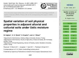
parameters that exhibited spatial structure, the selected model was fit using trial and error, as recommended by Clark (1979). All models, except the hole effect model, were fit to the experimental semivariograms. For the hole effect type of model, only a zone of influence was estimated. Representative semivariograms are illustrated in Fig. 2-4. Both measured and fitted -y*(h)'s are shown in Fig. 2 and 3 while only a measured (experimental) 7*(h) is shown in Fig. 4. The variability among the roughness parameters was described in terms of their spatial structure, i.e., spatial dependency among neighboring measurements of a particular parameter. In other words, the roughness parameter with the least spatial structure was the roughness parameter that varied the most in value from transect to adjacent transect across experimental plots. None of the measured parameters consistently exhibited spatial structure on all plots of the study. In this paper, an RP was considered to show spatial structure when its ZI was greater than 5 cm. Some roughness parameters, however, exhibited more spatial structure than others. The eight parameters were ranked in the following manner. First, the data were examined to determine whether or not each parameter
exhibited spatial structure on two or more of the four replications of each of the seven combinations of treatment and surface cover listed in Table 1. If a particular parameter was found to show spatial structure for a certain combination, an average ZI was calculated arithmetically by using the ZIs of the replications on which it was spatially dependent (Table 3). Second, the parameters were ranked according to the number of the seven combinations on which they exhibited spatial structure and then, for RPs showing spatial structure for the same number of combinations, according to the average ZIs calculated for each combination. Those parameters that showed the most spatial structure from transect to adjacent transect across a plot were MIOF and MIHT. The parameter that showed the least spatial structure (most variation from transect to transect) was PKHT. The parameters were ordered as MIOF > MIHT > MIF = DEDEP = FREQ = FHT = MI > PKHT . The semivariogram shape indices and ZIs measured for each of the eight roughness parameters appear in Table 3., While none of the parameters showed con-
316
SOIL SCI. SOC. AM. J., VOL. 52, 1988 2.0
2.0
PARAMETER DEDEP TRT. 1, REP. 2, VEG.
PARAMETER MIHT
••
1.5
TRT.3 , REP. 2 , BARE
• • • ••
ric
Co
0
0
10 20 40 30 50 DISTANCE, h (cm) Fig. 2. A spherical semivariogram measured and fitted (R 2 = 0.22) for the parameter DEDEP from Treatment 1, Replication 2, Vegetated subplot. The parameters for the fitted model were C = 9.92 x 10⁻² and a = 1.70 x ro l .
sistent spatial structure from plot to plot, within a plot numerous roughness parameters showing spatial structure were often found to have 7*(h)'s of the same shape, as in Treatment 1, Replication 2, Bare. Moreover, within a specific plot the zones of influence of the various spatially dependent RPs were often similar, as in Treatment 3, Replication 2, Veg. Zones of Influence
The zone of influence of all hole effect models was taken to be the first abscissa, a 1 , of Fig. 1C. Whenever a large clod was situated on the plot surface, the adjacent transects across the clod showed a similar (large) peak height, especially if the clod was relatively flat on its upper surface (as were most clods). If a zone of influence less than a l was chosen, then the large clod would influence the peak height measured on two (or more) transects. This obviously would make the peak height measured on those two transects dependent, rather than independent. Dependence caused by clods on the soil surface was considered detrimental to the roughness analysis. On the other hand, abscissa a, of Fig. 1C could be thought of as the average distance between large clods in a direction perpendicular to the transect. Dependence among transects with this dis4.0-
PARAMETER FHT TRT.
w
Ap o
X es, 2.0 41 E So I.0
o• o
•
+ ph
when hka
O•
3.0
•
2 (i hl when hca
h) r-c[E i
•
•
REP.4 , VEG.
• •
• •
•
•
•
I
I
I
20
30
40
DISTANCE 9
h (CM)
DISTANCE ,
I
I
30
40
1
50
h (cm)
Fig. 3. A linear semivariogram measured and fitted (R2 = 0.70) for the parameter MIHT from Treatment 3, Replication 2, Bare subplot. The parameters for the fitted model were C. = 6.70 x 10-' and p = 1.15 x 10⁻⁴.
tance as a ZI was not considered detrimental to the roughness analysis. Thus, ZIs were chosen equal to abscissa a, of Fig. 1C to eliminate dependence among transects caused by clods on the soil surface. The ZIs for each RP on each plot (Table 3) had physical significance. They were the distances h (Fig. 1A) beyond which the semivariance between measurements of an RP no longer increased. At distances h < a, the semivariance had not reached a maximum, suggesting that a measurement at one location was being influenced to some degree by a measurement at another location at a distance h from the first. The spacings within which measurements of an RP were dependent were taken to be the ZIs listed in Table 3. They appear to be of the appropriate magnitude. First, the diameters measured perpendicular to the transect of the largest clod present on the surface of each subplot ranged from 4.5 to 11.4 cm and averaged 7.7 cm. These values could be considered to be a first estimate of the zone of influence of a roughness parameter measured on a particular plot. In fact, the ZIs of Table 3 are of the same order of magnitude as this measurement. Second, previous research (ROmkens and Wang, 1986) has shown zones of influence for roughness parameters measured on a soil of similar texture ranging from 4 to 22 cm, with the upper limit corresponding to a chisel-disk tillage system that would likely leave the soil surface in a similar or even rougher condition as would the final cultivation of the chiseldisk-doall-cultivator tillage system used in this study. Thus, the ZIs listed in Table 3 appear to be realistic estimates of the distances on particular plots within
Roughness parameter
• I
I
20
Table 4. Average zones of influence for the eight roughness parameters when spatially dependent.
•
10
I
10
50
Fig. 4. A hole effect semivariogram measured fOr the parameter FHT from Treatment 1, Replication 4, Vegetated subplot.
Number of plots
Number of transects
Zone of influence, cm
PKHT
7
DEDEP
7
143 146 204 164 168 147 206 147
15.3 15.7 16.1 16.0 16.6 17.0 15.3 19.9
FREQ FHT MI MIHT MIOF MIF
10 8 8 7 10 7
LEHRSCH ET AL: SPATIAL VARIATION OF PARAMETERS DESCRIBING SOIL SURFACE ROUGHNESS
317
Table 5. The roughness parameterst by treatment and surface cover. Treatment*
0
1
2
3
Roughness parameter
Unit
Statistic
Bare',
Bare
Veg
Bare
Veg
Bare
Veg
PKHT
mm
DEDEP
mm
FREQ
mm-'
Mean 3E1 Mean SE Mean SE Mean SE Mean SE Mean SE Mean SE Mean SE
1.233 0.031 1.170 0.039 -1.520 0.006 -2.767 0.037 0.708 0.033 -0.529 0.006 2.238 0.038 -0.822 0.030
1.279 0.015 1.195 0.015 -1.473 0.011 -2.749 0.017 0.720 0.019 -0.569 0.006 2.189 0.023 -0.755 0.018
1.278 0.022 1.137 0.018 -1.490 0.012 -2.775 0.022 0.690 0.018 -0.584
1.240 0.016 1.155 0.013 -1.478 0.010 -2.715 0.017 0.687 0.016 -0.553 0.006 2.163 0.020 -0.788 0.016
1.225 0.018 1.163 0.013 -1.498 0.009 -2.730 0.022 0.680 0.017 -0.548 0.006 2.183 0.023 -0.826 0.018
1.269 0.018 1.164 0.015 -1.464 0.011 -2.734 0.020 0.684 0.021 -0.585 0.007 2.153 0.024 -0.788 0.023
1.199 0.018 1.145 0.017 -1.484 0.011 -2.680 0.020 0.648 0.019 -0.563 0.008 2.126 0.025 -0.844 0.020
FHT MI
mm' mm-'
MIHT MIOF
mm' mm-'
MIF
0.008
2.181 0.028 -0.796 0.016
t The values reported are those obtained by analyzing the roughness parameters after a common logarithmic transformation. * The statistics for Treatments 1, 2. and 3 were obtained using the appropriate error term from an analysis of variance for a split-plot design whereas the statistics for Treatment 0 were obtained using the error of its four replicates. The value of each replicate of each treatment was the arithmetic mean of spatially independent subsamples taken of that replicate. f Bare = bare subplot; Veg = vegetated subplot. 1 Standard error.
which the roughness parameters are spatially dependent. Semivariogram shape indices and ZIs averaged across replications are also given in Table 3. For lack of a better technique, the ZI of each of the linear •y*(1)'s of Table 3 was assumed to be either (i) less than the scale of measurement (5 cm) if no other RPs measured on that subplot exhibited spatial structure, or (ii) equal to the arithmetic mean of the ZIs of the spatially-dependent RPs measured on that subplot. It should be noted that roughness parameters measured on the vegetated subplots, rather than on the bare subplots, most often showed spatial structure. The zones of influence • from this 7(h) analysis thus reveal decreased variability (increased correlation) among the elevations of nearby points in the interrow zone subject to raindrop impact. As expected, over time from Treatment 1 to Treatment 3, for the most part the differences in ZIs between the bare and vegetated subplots within a cultivation either disappear or at least decrease (Table 3) as more and more of the subplot surface is protected by the soybean canopy. Somewhat surprising is the finding that for Treatment 2 (the second cultivation in the growing season), almost none of the RPs exhibited any spatial structure. The average ZIs for the eight roughness parameters
across all treatments (calculated using data only from plots on which they were spatially dependent) show surprising similarity (Table 4). While the averages were calculated only for ZI values greater than the scale of measurement (5 cm), the consistency among the computed averages was unexpected considering the wide variety of roughness parameters under study. These findings suggest that spatial dependence, if present in the measurements of any of the RPs, does not seem to exist at spacings of 20 cm or more. Roughness Parameters
Means for the roughness parameters by treatment and surface cover were estimated in the following manner. When a roughness parameter showed no spatial dependence on a particular plot (that is, on one of its replicates), its value for that replicate was calculated by arithmetically averaging the values from each of the 21 transects of that plot. When a parameter exhibited spatial dependence on a plot, however, its value for that plot was calculated using only a subset of the original 21 transects. For those plots, their ZI values (Table 3) were used to assemble subsets of independent transects. On such plots, a number of subsets were thus formed. The need was then to select a representative subset from among those formed. A
Table 6. The correlation coeffidentat between the roughness parameters.
Roughness parameter
Roughness parameter
PKHT
DEDEP
PKHT DEDEP FREQ FHT MI MIHT MIOF MIF
1.00 0.76** -0.08 -0.87** 0.88** -0.11 0.725* 0.895*
1.00 -0.38* -0.84** 0.91** 0.40* 0.85** 0.75!*
FREQ
FHT
MI
MINT
1.00 0.36 0.93** 0.87**
0.54**
MIOF
MIF
1.00 0.63**
1.00
1.00
0.54**
-0.37 -0.63** -0.68** 0.13
1.00 -0.93** -0.24
-0.94** -0.70**
1.00
0.07
*,** Significant at the 0.05 and 0.01 probability levels, respectively. t Simple correlation coefficients computed without regard to the structure in the data due to the split-plot design.
318
SOIL SCI. SOC. AM. J., VOL. 52,1988
subset could have been selected at random but preference was given to the subset whose mean for the parameter was closest to the mean for the parameter over the entire plot (ROmkens and Wang, 1987). The means reported in Table 5 are estimates of the means that would have been obtained had the design been balanced (that is, had the same number of transects been used to determine a roughness parameter's value for every plot) (SAS Institute Inc., 1982b).' They were calculated by first arithmetically averaging the spatially independent subsamples taken on each plot. Then in the subsequent analysis of variance, the means were weighted based upon the number of subsamples that were used to calculate each mean. Overall, within a treatment the means for vegetated plots were usually smaller than the means for the bare plots. This indicates that the parameters revealed the effects of the simulated rainfall that was applied to the vegetated plots but not to the bare plots. The effects of cultivation (treatment) on the bare-plot means for each parameter were inconsistent. The effects of cultivation and surface cover on all eight roughness parameters will be discussed in more detail in a subsequent manuscript. The effects of cultivation on the MIF parameter alone have been described elsewhere (Lehrsch et al., 1987). The variability among replications was not great (Table 5). The parameter that showed the least variation from replication to replication was FREQ. On the other hand, the parameter that showed the most variation was MI, followed by MIF. Even so, no mean had a coefficient of variation (CV) over 10% while nearly 84% of the means had CVs under 5%. The correlation coefficients between the roughness parameters (Table 6) reveal interesting information. PKHT and DEDEP, being measures of a transect's maximum and minimum elevations, respectively, were correlated positively since both would tend to be large on a roughly tilled surface, such as after primary tillage. MI also seems to be a sensitive indicator of roughened surfaces as it is well correlated to PKHT and DEDEP. MI, however, also supplies information on elevations all along a transect yet is responding nearly as much as PKHT and DEDEP to extremes in elevation. MI was not correlated to FREQ. Thus, each appears to be a measure of a particular aspect of surface roughness that is not measured by the other. Hence, the parameter MIOF or MIF that incorporates information from two such statistically independent aspects of roughness may be a promising descriptor of soil surface roughness. Research is continuing to identify such a roughness descriptor from among the eight parameters examined in this study. The findings of this study have implications for future research. First, the frequency distributions of roughness parameters should be examined. As found in this study, roughness parameters in certain situations may not be normally distributed. Second, the roughness parameters were often spatially independent but not always, however. To insure independent observations, spatial structure should be investigated using semivariograms or autocorrelation analyses. In this study, spatial dependency did not appear to be associated with any particular roughness parameter.
Vegetated plots subjected to artificial rainfall, however, were often found to have spatially dependent roughness parameters (Table 3). Third, when spatial dependency was present, in general it did not appear to exist at spacings of 20 cm or more. In future experiments similar to this one, however, measurements should not be spaced 20 cm or more apart if spatial structure is not present; far too much information on surface roughness would thereby be ignored. Transect spacing to insure independent observations has been found to be dependent upon the tillage method used (ROmkens and Wang, 1986). Fourth, in future studies roughness parameters should be measured on more than 21 transects per plot using either larger plots or a closer spacing between transects. The resultant semivariograms would then be better defined and the zones of influence more reliable. Finally, hole effect semivariograms may be more common for some soil properties than once thought. Hole effect semivariograms can reveal information on the periodicity associated with the spatial measurements of soil properties. CONCLUSIONS
The eight parameters describing soil surface roughness were found most commonly to be spatially independent, that is, to have experimental semivariograms revealing a nugget effect. In over two-thirds of the cases, no spatial dependency was evident. On the other hand, when a roughness parameter was spatially dependent, its semivariogram usually was either spherical, linear with a nugget constant, or exhibited a hole effect. The hole effect model was predominant, being identified in just over one-half of the semivariograms that revealed spatial structure. The zones of influence of the semivariograms for the roughness parameters when spatially dependent averaged 15 to 20 cm. REFERENCES Allmaras, R.R., R.E. Burwell, W.E. Larson, R.F. Holt, and W.W. Nelson. 1966. Total porosity and random roughness of the interrow zone as influenced by tillage. USDA Conserv. Res. Report no. 7. U. S. Gov. Print. Office, Washington, DC. Burwell, R.E., R.R. Allmaras, and M. Amemiya. 1963. A field measurement of total porosity and surface microrelief of soils. Soil Sci. Soc. Am. Proc. 27:697-700. Clark, I. 1979. Practical geostatistics. Applied Science Publishers Ltd., London. Conover, W.J. 1971. Practical nonparametric statistics. John Wiley & Sons, Inc., New York. Davis, J.C. 1973. Statistics and data analysis in geology. John Wiley & Sons, Inc., New York. Fehr, W.R., C.E. Caviness, D.T. Burmood, and J.S. Pennington. 1971. Stages of development descriptions for soybeans, Glycine max (L.) Merrill. Crop Sci. 11:929-931. Gem, Y.M., A.W. Warrick, and D.E. Myers. 1981. Spatial dependence of physical properties of a Typic Torrifluvent soil. Soil Sci. Soc. Am. J. 45:709-715. Garber, M.C. 1973. Soil survey of Lee County, Mississippi. USDASCS, Mississippi Agric. Exp. Stn. U. S. Gov . Print. Office, Washington, DC. Journel, A.G., and Ch.J. Huijbregts. 1978. Mining geostatistics. Academic Press, New York. Kuipers, M. 1957. A relief meter for soil cultivation studies. Neth. J. Agic. Sci. 5:255-262. Lehrsch, G.A., F.D. Whisler, and M.J.M. Ramkens. 1987. Soil surface roughness as influenced by selected soil physical properties. Soil Tillage Res. 10:197-212. Meyer, L.D., and W.C. Harmon. 1979. Multiple-intensity rainfall
LEHRSCH ET AL: SPATIAL VARIATION OF PARAMETERS DESCRIBING SOIL SURFACE ROUGHNESS simulator for erosion research on row sideslopes. Trans. ASAE 22:100-103. Myhre, D.L., and J.O. Sanford. 1972. Soil surface roughness and straw mulch for maximum beneficial use of rainfall by corn on a blackland soil. Soil Sci. 114:373-379. ROmkens, M.J.M., S. Singarayar, and C.J. Gantzer. 1986. An automated noncontact surface profile meter. Soil Tillage Res. 6:193202. ROmkens, M.J.M., and J.Y. Wang. 1986. Effect of tillage on surface
319
roughness. Trans. ASAE 29:429-433. R6mkens, M.J.M., and J.Y. Wang 1987. Soil roughness changes from rainfall. Trans. ASAE 30:101-107. SAS Institute Inc. 1982a. SAS user's guide: Basics. 1982 ed. SAS Inst., Inc., Cary, NC. SAS Institute Inc. 1982b. SAS user's guide: Statistics. 1982 ed. SAS Inst., Inc., Cary, NC. Steel, R.G.D., and J.H. Torrie. 1960. Principles and procedures of statistics. McGraw-Hill Book Co., Inc., New York.