Spatial vs. non-spatial eco-evolutionary dynamics in a ...

Spatial vs. non-spatial eco-evolutionary dynamics in a tumor growth model Li Youa , Joel S. Brownc,d , Frank Thuijsmana , Jessica J. Cunninghamd , Robert A. Gatenbyd,e , Jingsong Zhangf , Kateˇrina Staˇ nkov´aa,b,∗ a Department

of Data Science and Knowledge Engineering, Maastricht University, Maastricht, The Netherlands Institute of Applied Mathematics, Technical University Delft, Delft, The Netherlands c Department of Biological Sciences, University of Illinois at Chicago, Chicago, Illinois, USA d Department of Integrated Mathematical Oncology, Moffitt Cancer Center & Research Institute, Tampa, Florida, USA e Department of Diagnostic Imaging and Interventional Radiology, Moffitt Cancer Center & Research Institute, Tampa, Florida, USA f Department of Genitourinary Oncology, Moffitt Cancer Center & Research Institute, Tampa, Florida USA b Delft

Abstract Metastatic prostate cancer is initially treated with androgen deprivation therapy (ADT). However, resistance typically develops in about 1 year – a clinical condition termed metastatic castrateresistant prostate cancer (mCRPC). We develop and investigate a spatial game (agent based continuous space) of mCRPC that considers three distinct cancer cell types: 1) those dependent on exogenous testosterone (T + ), 2) those with increased CYP17A expression that produce testosterone and provide it to the environment as a public good (T P ), and 3) those independent of testosterone (T − ). The interactions within and between cancer cell types can be represented by a 3 × 3 matrix. Based on the known biology of this cancer there are 22 potential matrices that give roughly three major outcomes depending upon the absence (good prognosis), near absence or high frequency (poor prognosis) of T − cells at the evolutionarily stable strategy (ESS). When just two cell types coexist the spatial game faithfully reproduces the ESS of the corresponding matrix game. With three cell types divergences occur, in some cases just two strategies coexist in the spatial game even as a non-spatial matrix game supports all three. Discrepancies between the spatial game and non-spatial ESS happen because different cell types become more or less clumped in the spatial game – leading to non-random assortative interactions between cell types. Three key spatial scales influence the distribution and abundance of cell types in the spatial game: i. Increasing the radius at which cells interact with each other can lead to higher clumping of each type, ii. Increasing the radius at which cells experience limits to population growth can cause densely packed tumor clusters in space, iii. Increasing the dispersal radius of daughter cells promotes increased mixing of cell types. To our knowledge the effects of these spatial scales on eco-evolutionary dynamics have not been explored in cancer models. The fact that cancer interactions are spatially explicit and that our spatial game of mCRPC provides in general different outcomes than the non-spatial game might suggest that non-spatial models are insufficient for capturing key elements of tumorigenesis. Keywords: Prostate Cancer, Evolutionary Game Theory, Spatial Game, Non-spatial Game

1. Introduction In cancer biology, tumors are viewed as complex ecosystems consisting of cancer cells, normal cells, blood vasculature, inter-cellular spaces, and various nutrients such as oxygen and glucose [1, ∗ Corresponding

author Email address: [email protected] (Kateˇrina Staˇ nkov´ a)

Preprint submitted to Journal of Theoretical Biology

September 1, 2017

5

10

15

20

25

30

35

40

45

50

55

2, 3]. Within this ecosystem, cancer cells, often of distinct types, compete for space and nutrients, and engage in direct interactions. Cancer cells both contribute towards and are affected by their neighborhoods (known as microenvironments) within which they consume available resources, survive and proliferate [4]. Within these neighborhoods there are eco-evolutionary feedbacks where limiting resources influence the total abundance of cancer cells and interactions between tumor cells influence the frequency of cell types. While often modeled non-spatially, several features of tumors invite spatially-explicit models. For instance, biopsies, histological samples and MRI imaging all provide spatial information on tumor characteristics [5, 6]. Pathologists often measure and score spatial distributions of cancer cell types, vasculature, immune cells, and other tumor properties [7, 8]. Finally, increasingly cancer biologists recognize the ubiquity of spatial heterogeneity within tumors [9, 10]. This heterogeneity likely has significance for tumor progression, metastases and patient outcome [11]. Mathematical models of cancer have been employed to understand tumor initiation, progression and metastases [12]. Such models can be used to fit existing data, evaluate key factors relevant to cancer progression, or provide qualitative and quantitative predictions that can be experimentally validated [13, 14]. Non-spatial models of cancer can be deterministic or stochastic. They can take the form of ordinary differential equations that track the dynamics of the cancer cells (often seen as growing logistically or according to a Gompertz equation [15]) and perhaps that of normal cells and/or immune cells. Spatially explicit models may take the form of diffusion processes framed as partial differential equations models [16], or the models may be agent based [17]. As agent based models, the cancer cells or other features of the tumor may be represented on vertices of a lattice or network. Or, individual cells may occupy a space on a spatial grid described as squares or hexagons [18, 19]. Finally, agent based models can consider continuous space where the cancer cells are represented by continuously varying spatial coordinates in one, two or three dimensions [20]. Mathematical models can consider the eco-evolutionary dynamics that occur in tumors. Here we define a cancer cell “type” as cells that share the same heritable phenotype relevant to the cancer under study. Ecological dynamics represent changes in the population size or density of cancer cells. The evolutionary dynamics consider how the heritable traits of cancer cell lineages change with time, or how the frequencies of different cancer cell types change with time. When a cancer cell’s survival or proliferation probabilities are influenced by its type and the types of other cancer cells, the dynamics are frequency-dependent and therefore can be described using game theory. Evolutionary game theory (EGT) provides an excellent modeling tool for considering complex tumors that include several interacting cancer cell types. EGT deals with interactions between players [21, 22]. As a game, cancer cells represent the players, their types or heritable phenotypes represent the different strategies, and survival and proliferation rates represent the payoffs. A cell’s payoff will be influenced by its strategy and the strategies of others. EGT includes tools for modeling population dynamics and the evolutionary dynamics of changes in the frequency of different cancer cell types. EGT can be used to find ecoevolutionary equilibria and to evaluate their stability. When there are a finite number of different possible strategies among the cancer cells, then the evolutionary dynamics can be modeled using replicator dynamics (RD) [23]. RD are non-spatial and apply when an individual interacts with the population at large either via random interactions or through “playing the (entire) field”. Recent research has focused on extending RD into spatially explicit scenarios [24, 25, 26]. Both the evolutionary dynamics and subsequent equilibria may change when space is made explicit [27, 28, 29, 30, 31]. Recently, cancer has been modeled using replicator dynamics. These models have either been non-spatial [32, 33, 34] or spatially defined as occurring on a fixed lattice of a graph [35]. Here we use a spatially-explicit agent based approach to model cancer as an evolutionary game. First, we describe metastatic castrate-resistant prostate cancer that provides the motivation for our modeling work. The biology of this cancer suggests three important cancer cell types (strategies) whose interactions and payoffs can be described with a 3 × 3 matrix game. We can analyze this matrix game as a non-spatial model using RD, and we develop a spatial version of the 2

60

65

70

75

prostate cancer model where the space is continuous. Second, we find the evolutionarily stable strategies (ESS) for the non-spatial game, and the stable equilibria that arise in the spatial variant of the model. Finally, using the spatial model, we explore three relevant processes and scale dependencies that must occur in actual tumors. To our knowledge these processes and their interactions have not been collectively explored in cancer models. The first of these processes relates to the density-dependence radius. A given tumor cell will be negatively affected by the density of other cancer cells within some neighborhood that represents the local depletion of resources or buildup of toxins. The second process relates to the frequency-dependence radius, that describes the distance at which cancer cells play the game. Up to what distance does the strategy of neighbors matter in terms of influencing the payoff to an individual tumor cell? The third process relates to the dispersal radius. Cancer cells exhibit motility and the resulting movement of cells determines the distance between two daughter cells. Prior models have not made the distinction between the three scale dependent processes of density-dependence, frequency-dependence, and dispersal radius. By considering continuous space, our model lends itself to examining the effects of these three scale-dependent processes on the eco-evolutionary equilibrium and on the dispersion of cancer cells and strategies in space. In what follows we introduce the metastatic castrate-resistant prostate cancer models used in this paper (Section 2); we compare the eco-evolutionary outcomes of the non-spatial and spatial models (Section 3); we examine the effects of varying the three scale-dependent processes on spatial equilibria (Sections 4); and we discuss our results and highlight some directions for future research (Section 5). 2. Models: Replicator dynamics and its spatial variant 2.1. Background: Metastatic castrate-resistant prostate cancer

80

85

90

95

100

105

Prostate cancer most commonly metastasizes to the bone and several to a dozen or more secondary tumors can arise across bones of a single patient [33, 36]. Despite no longer residing within the primary tumor of the prostate (in fact for many of these patients the prostate may have been removed), these cancer cells still retain androgen receptors and rely on testosterone produced by normal cells of the patient and distributed through the blood [37]. We shall refer to this cancer cell type as having strategy T + . To target these cancer cells’ need for testosterone, androgen deprivation therapy (ADT) stops normal production of testosterone in the patient – a treatment termed “chemical castration” [38, 39, 40]. Virtually all patients initially respond to ADT. But, metastatic prostate cancer remains an almost uniformly fatal disease because the cancer cells are able to evolve resistance. In ADT, resistance typically results in a few months or years and the disease progresses to metastatic castrate-resistant prostate cancer (mCRPC). Resistance to ADT typically occurs through two different strategies. One of these involves the upregulation of CYP17A whereby the cancer cell produces its own testosterone [41, 42]. These we shall refer to as T P cells. They retain androgen receptors. The T P cells have the side effect of providing testosterone to their external environment where it becomes available to T + cells. Finally, resistance to androgen deprivation can take the form of cancer cells becoming wholly independent of testosterone: T − . Treatment of mCRPC depends on the dominant resistance strategy. When T P cells are that largest intratumoral population, abiraterone, a CYP17A inhibitor, is typically effective. However, even in patients who respond to abiraterone, the disease progresses usually within 1-2 years. Here we investigate the eco-evolutionary dynamics of mCRPC by modeling the composition and dispersion patterns of the three cell types (T + , T P and T − ) within a tumor. The resulting eco-evolutionary equilibria become important in that a tumor with primarily T + and T P cells can be effectively treated with drugs such as abiraterone that target androgen receptors [43]. However, tumors with high frequencies of T − cells will be unresponsive to abiraterone and require chemotherapy.

3

2.2. Model basics

110

Let T = {T + , T P , T − } be the set of cell types from Section 2.1. Let xi , i ∈ T, denote the frequency of the cells of type i ∈ T in the population. We assume that the cancer cells interact with each other as a game. When a focal cell of type i ∈ T interacts with a cell of type j ∈ T , the outcome is the probability that the focal cell divides and creates an offspring of type i. These division probabilities for interaction between all types form a payoff (fitness) matrix A depicted in Table 1. Please consult Appendix A for details about the non-spatial model corresponding to this payoff matrix. +

T TP T−

T+ 0 c e

TP a 0 f

T− b d 0

Table 1: The fitness matrix for T + , T P and T − cell populations. The diagonal values have been set to 0.

2.3. Replicator dynamics in metastatic castrate-resistant prostate cancer For each type i ∈ T, the replicator dynamics [23] define the time change x˙ i of its cell frequency xi : x˙ i = xi (ei A x> − x A x> ), 115

120

125

130

i∈T

(1)

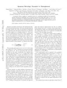
where x = (xT + , xT P , xT − ), and ei is the i-th row of a 3 × 3 identity matrix. Even with the same initial conditions (x(0) = x0 ), the frequency dynamics (1) will vary with the payoff matrix A. For the 22 cases, we can map the frequency trajectories and the evolutionary stable strategies (ESSs) on a simplex (Figure 1). When starting from positive initial frequencies, i.e., x(0) = (1/3, 1/3, 1/3) , each case of our model results in a single ESS, which is the attractor for the dynamics given by (1). In the notation of Bomze [44], the games we consider fall into the following two groups: (i) “no fixed point in the interior simplex” and “no edge pointwise fixed”; and (ii) they will exhibit “one fixed point in interior simplex” and “three non-corner fixed points on edges”. Based on the frequency of the T − cells at the ESS, we can divide the 22 cases for replicator dynamics into three different groups (Table 2): I. (positive) The ESS frequency of T − cells is 0 – such tumors should respond strongly to abiraterone II. (neutral) The ESS frequency of T − cells is between 0 and 0.15 – such tumors may respond to abiraterone III. (negative) The ESS frequency of T − cells is greater than 0.15 – such tumors may correspond to non-responders 2.4. Spatial replicator dynamics in metastatic castrate-resistant prostate cancer

135

140

In this section, we model the density and frequency dynamics of the prostate cancer cells as a spatial game on a continuous space. We imagine the cancer cells as players on a torus Θ = [0, 50) × [0, 50) with periodic boundary conditions. Rather than having a fixed grid or lattice, cells can exist at any point on this surface. Initially, there are 99 cancer cells (33 of each type), scattered randomly within the central zone C = [20, 30] × [20, 30] of the flat torus Θ. For the spatial game we specify rules regarding cell death, density-dependent interactions, frequency-dependent interactions and cell proliferation, which occur in generations. During a generation all living cells are selected in a random order to undergo the following actions:

4

Figure 1: The trajectories of cell type frequencies for each matrix from Table 2, ordered by group. The vertices of the simplex correspond to a frequency of 1 for the corresponding cell type. The red dots represent the ESS’s and the black dots represent the saddle points.

5

#

(a, b, c, d, e, f )

ESS

1

(0.6,0.3,0.5,0.4,0.2,0.1)

6 5 ( 11 , 11 ,0)

2

(0.6,0.2,0.5,0.3,0.4,0.1)

6 5 , 11 ,0) ( 11

3

(0.6,0.2,0.5,0.4,0.3,0.1)

6 5 ( 11 , 11 ,0)

4

(0.5,0.3,0.6,0.4,0.2,0.1)

5 6 ( 11 , 11 ,0)

5

(0.5,0.2,0.6,0.3,0.4,0.1)

5 6 , 11 ,0) ( 11

6

(0.5,0.2,0.6,0.4,0.3,0.1)

5 6 ( 11 , 11 ,0)

7

(0.4,0.3,0.6,0.5,0.2,0.1)

( 25 , 35 ,0)

9

(0.4,0.2,0.6,0.5,0.3,0.1)

( 25 , 35 ,0)

11

(0.3,0.2,0.6,0.5,0.4,0.1)

( 13 , 23 ,0)

14

(0.6,0.1,0.5,0.4,0.3,0.2)

6 5 , 11 ,0) ( 11

17

(0.5,0.1,0.6,0.4,0.3,0.2)

5 6 ( 11 , 11 ,0)

20

(0.4,0.1,0.6,0.5,0.3,0.2)

( 25 , 35 ,0)

8

(0.4,0.2,0.6,0.3,0.5,0.1)

( 11 , 17 , 2 ) 30 30 30

10

(0.3,0.2,0.6,0.4,0.5,0.1)

( 10 , 22 , 3 ) 35 35 35

12

(0.6,0.1,0.5,0.3,0.4,0.2)

( 14 , 13 , 4 ) 31 31 31

15

(0.5,0.1,0.6,0.3,0.4,0.2)

( 11 , 14 , 2 ) 27 27 27

13

(0.6,0.1,0.5,0.2,0.4,0.3)

( 13 , 13 , 13 )

16

(0.5,0.1,0.6,0.2,0.4,0.3)

7 10 8 ( 25 , 25 , 25 )

18

(0.4,0.1,0.6,0.3,0.5,0.2)

( 14 , 24 , 14 )

19

(0.4,0.1,0.6,0.2,0.5,0.3)

5 11 14 ( 30 , 30 , 30 )

21

(0.3,0.1,0.6,0.4,0.5,0.2)

2 7 3 ( 12 , 12 , 12 )

22

(0.3,0.1,0.6,0.5,0.4,0.2)

7 22 6 ( 35 , 35 , 35 )

Group

I (positive)

II (neutral)

III (negative)

Table 2: Division of the 22 cases for replicator dynamics (3) into 3 groups according to the ESS frequencies of T − cells. No T − cells (group I) indicate a highly treatable tumor, a low frequency of T − cells indicates a moderately treatable tumor (group II), while a high frequency of T − cells (group III) indicates an untreatable tumor (non-responders).

145

Cell death. We imagine that cell death can be either stochastic or deterministic. A cancer cell dies with either a fixed probability (stochastic) or after a fixed number of generations (deterministic). If the focal cell dies, it does not undergo any further actions. Following death, the cell either stays in the field permanently or is removed after a pre-specified number of generations. The combinations of deterministic or stochastic cell death and the rate at which dead cells stay in the field (5 generations, 30 generations, or permanently) generate six possible mortality regimes (see Table 3). If the focal cell remains alive, it undergoes the next action. Scenario 1 2 3 4 5 6

Mortality regime Cell death Dead cells staying in field Stochastic (probability 5%) Short (5 generations) Deterministic (20 generations) Permanently Stochastic (probability 5%) Permanently Deterministic (20 generations) Long (30 generations) Deterministic (20 generations) Short (5 generations) Stochastic (probability 5%) Long (30 generations)

Table 3: Six scenarios corresponding to six mortality regimes

6

155

Density-dependent cell interactions. We imagine that available space and resources are necessary for successful cell proliferation. We define the density-dependence neighborhood as a disc around the focal cell with a pre-specified radius, called the density-dependence radius (Figure 2a). If the number of cells (itself and dead cells included) within this density-dependence neighborhood is greater than or equal to 10 cells per unit area, then the focal cell cannot proliferate and it does not move onto additional actions in the current generation. If the density of cells within the density-dependence neighborhood is less than 10 cells per unit area then the focal cell moves onto the next action.

160

Frequency-dependent cell interactions. We imagine the cells also have a frequency-dependence neighborhood, which is a disc around the focal cell with a pre-specified radius, called the frequencydependence radius (Figure 2b). The focal cell randomly selects a neighbor cell from the living cells occurring within this frequency-dependence neighborhood. Having selected the focal cell’s “opponent” for the game we move to the last action.

150

165

Cell proliferation. The probability of the focal cell undergoing cell division and producing a daughter cell is determined by the payoff from the matrix A if we let the type of the focal cell be the row strategy and the type of the opponent be the column strategy (Table 1). If the focal cell reproduces, it generates a daughter cell of its own type. This daughter cell is not placed in the field immediately, but only after all living cells have completed their actions for the current generation. A given daughter cell is placed at a random location in the focal cell’s dispersal neighborhood (Figure 2c). The dispersal neighborhood is a disc around the focal cell with pre-specified radius, called the dispersal radius.

(a)

(b)

(c)

Figure 2: A focal cell and its three neighborhoods. (a) Density-dependence neighborhood. A focal cell might proliferate if the density of cells within the disc defined by the density-dependence radius is below a threshold. (b) Frequency-dependence neighborhood. The focal cell’s likelihood of proliferating will be determined from an interaction between it and a randomly selected cell from within the disc defined by the frequency-dependence radius. (c) Dispersal neighborhood. If a focal cell proliferates, its daughter cell is placed randomly within the disc defined by the dispersal radius. 3. Tumor growth and composition 170

175

In this section we simulate tumor growth under the six different mortality regimes (Table 3). We compare the tumor composition of the six scenarios with the ESS of the non-spatial models for the 22 payoff matrices. In the simulations we track changes in 1. the total number of cancer cells (population dynamics) 2. the frequencies of cell types (frequency dynamics) 3. the dispersion pattern of each cell type

7

180

185

Each simulation begins with 99 cells (33 per cell type), placed randomly in the central 10 × 10 zone of the flat torus Θ = [0, 50) × [0, 50). We ran simulations for 2000 generations. For each combination of the mortality regime (Table 3) and payoff matrix we repeated the simulation five times. This resulted in 660 simulations. For these simulations, we set the density-dependence, frequency-dependence, and dispersal radii to one. The density threshold for reproduction was set to 10 cells per unit area within the focal cell’s density-dependence neighborhood. To evaluate the spatial dynamics and for comparisons to the ESS of the non-spatial model, we need stability concepts for spatial equilibria in terms of the densities and frequencies of the three cell types. Here, we will consider a spatial equilibrium stable if the frequencies in each two consecutive generations have a difference less than 0.001 in the 50 past generations, as stated formally in Definitions 3.1 and 3.2: Definition 3.1 (Stable frequency in the spatial game). Frequency xi of type i ∈ T is stable in generation τ if |xi (t + 1) − xi (t)| ≤ 0.001 for all generations t ∈ {τ − 49, τ − 48, ..., τ }.

190

195

200

Definition 3.2 (Stable spatial equilibrium). A spatial equilibrium is stable in generation τ if the frequencies of all three types (T + , T P , T − ) are stable in this generation. In the reminder of the paper, whenever we refer to “equilibria”, what we mean is “stable equilibria”, just to simplify the notation. We might be able to observe two different types of (stable) equilibria: The transient (stable) equilibrium and saturated (stable) equilibrium. The former might occur when the total number of tumor cells is still growing, while the latter occurs once the space is saturated, i.e., once the total population of living cells as well as populations per type in the tumor do not change (due to the finite size of the field Θ). In order to quantify when such equilibria occur, we define the transient and saturated equilibria in Definitions 3.3 and 3.4. Definition 3.3 (Transient stable spatial equilibrium). A stable spatial equilibrium in generation τ is called transient if the sum of populations of T + , T P , and T − cells keeps growing in generations {τ − 49, τ − 48, ..., τ }. In the following definition, we use the term maximal total population, which refers to the largest total population of cells reached over the run of the simulation, including both dead and living cells in this count.

205

Definition 3.4 (Saturated stable spatial equilibrium). A stable spatial equilibrium in generation τ is called saturated if the total cell population stays within 1 % of its maximal population size in generations {τ − 49, τ − 48, ..., τ }. 3.1. The effects of the mortality regime on tumor growth

210

215

220

Whether death is stochastic or deterministic and how long dead cells remain in the tumor strongly influence both the transient and saturated spatial equilibria. Figure 3 shows the spatial dynamics of matrix #19 for each scenario from Table 3. By generation 200 for matrix #19, the frequencies of cell types have reached transient equilibria in all scenarios even as the entire space has yet to be filled (Figure 4). In scenario 1 (mortality regime: stochastic death and removal of dead cells after 5 generations) we observe that T + , T P , and T − cells are rather well mixed with dead cells and the tumor is tightly packed throughout. A similar tumor is observed in scenario 5 (mortality regime: deterministic death after 20 generations and removal of dead cells after 5 generations) and scenario 6 (mortality regime: 5% stochastic death and removal of dead cells after 30 generations), while more dead cells are observed in the field in scenario 6 (with ≈ 60% cells dead) than in scenario 1 (with ≈ 20% cells dead) and scenario 5 (with ≈ 22% cells dead). In scenario 2 (mortality regime: deterministic death and no removal of dead cells) we see the formation of a necrotic core of densely packed dead cells. Scenario 3 (mortality regime: 5% stochastic death rate and no removal of dead cells) is similar to scenario 2, except that a 8

(a)

(b)

(c)

(d)

(e)

(f)

Figure 3: Transient and saturated equilibria corresponding to the six different mortality regimes (Table 3). This example uses payoff matrix #19. The generations depicting stable transient/saturated equilibria are marked in gray. Scenarios 2 and 3 have no stable saturated equilibria as all cells die when saturation is reached. Each panel shows the frequencies of the three cell types over the course of 2000 generations.

225

230

small number of living cells persist within the necrotic core. In scenario 4 (mortality regime: deterministic death and removal of dead cells after 30 generations) the tumor becomes a ring with an outer surface of living cells, an inner surface of dead cells and bulges of living cells recolonizing an otherwise empty center. Figure 5 illustrates the tumors at their saturated equilibria for the six scenarios using payoff matrix #19. In scenarios 1 and 4 the living cells of the three types are relatively well mixed. In scenario 1 the entire space is filled. Dead cells are mixed with the living ones and the appearance is similar to the transient equilibrium. In scenario 4 the ring shape of the tumor progresses to a more patchy distribution of living and dead cells surrounding patches of empty space. Scenarios 2 and 3 (no removal of dead cells) result in the filling of the space with dead cells.

9

(a)

(b)

(c)

(d)

(e)

(f)

Figure 4: Tumors in space at the point where cell type frequencies achieve a stable transient equilibria. Subfigures (a), (b), (c), (d), (e) and (f) correspond to scenarios 1, 2, 3, 4, 5 and 6 in Table 3, respectively, with payoff matrix #19. T + , T P , T − and dead cells are denoted by blue, red, green and black color, respectively.

(a)

(b)

(c)

(d)

(e)

(f)

Figure 5: Tumors in space at the point where cell type frequencies achieve stable saturated equilibria. Subfigures (a), (b), (c), (d), (e) and (f) correspond to scenarios 1, 2, 3, 4, 5 and 6 in Table 3, respectively, with payoff matrix #19. T + , T P , T − and dead cells are denoted by blue, red, green and black color, respectively.

235

Tables 5, 6 and 7 (in Appendix C) record the transient and saturated equilibrium frequencies of the three cell types for all six scenarios and for all 22 payoff matrices, respectively. Based on the six scenarios and the twenty-two possible arrangements of payoff matrices, we observe the following: 10

240

• In scenario 1 (mortality regime: 5% stochastic death rate and removal of dead cells after 5 generations), the transient and saturated equilibrium frequencies for matrices from group I (positive) are very close to the matrix game ESS, while their equilibrium frequencies for matrices from group II (neutral) and III (negative) deviate from the matrix game ESS. In conclusion, when the ESS for the matrix game contains just two cell types (T + and T P ), the spatial model yields cell type frequencies near identical to this ESS. When the ESS of the matrix game contains all three cell types, the spatial game results in equilibrium cell type frequencies quite different than the non-spatial ESS.

255

• In scenario 2 (mortality regime: deterministic death after 20 generations and no removal of dead cells), the transient equilibrium frequencies for matrices from group I (positive) are close to the ESS while the transient equilibrium frequencies for matrices from group II (neutral) and III (negative) deviate substantially from the non-spatial ESS. For matrices in group II, T − cells die out during the transient equilibrium, and the frequencies of T + and T P cells converge on the 2-strategy non-spatial equilibrium if only T + and T P exist. For the matrices in group III, the transient equilibrium frequency of T − is much lower, and the frequencies of T + and T P cells are higher than the non-spatial ESS. There is no stable saturated equilibrium as all cells die when the space is filled no matter which matrix is examined. This is due to the existence of the necrotic core, which keeps spreading and eventually takes over the entire field.

260

• In scenario 3 (mortality regime: 5% stochastic death rate and no removal of dead cells), the equilibrium frequencies are quite similar to those in scenario 2. The necrotic core eventually takes over the space. While some living cells do survive for many generations, they eventually fail to proliferate as they become surrounded by dead cells. Eventually, all cells die.

245

250

265

270

275

280

285

• In scenario 4 (mortality regime: deterministic death after 20 generations and removal of dead cells after 30 generations), the transient equilibrium frequencies are quite similar to these in scenarios 2 and 3. For matrices from group I (positive) the frequencies of T + and T P cells are close to the ESS (T − are absent from the ESS); for matrices from group II (neutral) T − cells die off leaving a transient equilibrium with just T + and T P cells close to their 2-strategy ESS. For matrices in group III, T − cells persist but have much lower frequencies than predicted by the ESS. For all matrices and mortality regimes the transient phase sees a tumor that grows as an expanding ring. Living cells inhabit the outer edge of the ring and dead cells the inner edge. At the saturated equilibrium the thickness of the dead cells on the ring influences the spatial dynamics and cell type frequencies. A thinner ring of dead cells during the transient phase permits live cells to recolonize the empty space inside the ring, giving rise to a saturated equilibrium as shown in Figure 5d. A thicker band of dead cells results in a tumor at saturation that has large empty spaces and a relatively low number of living cells. The frequencies of cell types at the saturated equilibria for matrices from group I (positive) and matrices #8, #12 and #15 deviate substantially from the non-spatial ESS as clumps of living cells become separated and patchy due to the large empty spaces within the tumor. The saturated equilibrium frequencies for the remaining matrices are close to a 2-strategy ESS, as either T + or T − dies out; T P cells occur at higher frequencies than expected by the ESS for all matrices in groups II and III. • In scenario 5 (mortality regime: deterministic death after 20 generations and removal of dead cells after 5 generations), the transient equilibrium frequencies as well as the saturated equilibrium frequencies are very close to those generated from scenario 1. • In scenario 6 (mortality regime: 5% stochastic death rate and removal of dead cells after 30 generations), the transient and saturated equilibrium frequencies for matrices from group I (positive) are close to the ESS, while their equilibrium frequencies for matrices from group II (neutral) and III (negative) deviate from the ESS. 11

290

295

300

The mortality regime is paramount in determining tumor architecture. With no removal of dead cells (scenarios 2 & 3), the space becomes filled with dead cells and the ultimate survival of the tumor would require unbounded space for living cancer cells to invade. When dead cells take a long time to disappear, the tumor exhibits rings of living cells surrounding necrotic regions, the tumor dies off (scenario 4), or dead cells represent over half of those visible in the tumor (scenario 6). The arrangement of these empty patches within the tumor becomes dynamic as some patches become colonized by living cells and new empty patches form. Regardless, the overall abundance of live cancer cells is much reduced because of the empty spaces and the long persistence of dead cells. If dead cells persist for only a short number of generations (scenario 1 & 5) the tumor grows and fills the entire space as a contiguous population of living cells. The living cells both expand along the margin of the tumor and continually repopulate the core of the tumor as cells die and disappear. The saturated equilibria in scenario 1 result in high and persistent populations of cancer cells; though the mosaic of cell types changes constantly at small spatial scales. 3.2. Spatial vs. non-spatial dynamics

305

To compare in more detail the dynamics and equilibria of the spatial versus non-spatial models, we consider the saturated equilibria for the 22 payoff matrices under just the first scenario (stochastic mortality and short duration before removing dead cells). This scenario produces a highly dynamic tumor that saturates at dense populations of living cells. We focus on the three important themes in tumorigenesis: 1. the population size of live cancer cells at the saturated equilibrium 2. the frequencies of cell types at the saturated equilibrium 3. the dispersion patterns of cell types within the tumor To measure the dispersion pattern of a given cell type within the saturated tumor, we use the variance-to-mean ratio [45]. The variance-to-mean ratio of type i ∈ T is defined as N P

ρi = 310

315

320

325

(nki − n ¯ i )2

k=1

(N − 1)¯ ni

(2)

where the space is evenly divided into N = 900 subsquares. Varying the number of subsquares a bit gives us qualitatively similar results, therefore we consider N = 900 as being representative. Quantity nki is the number of type i cells in the k-th subsquare and n ¯ i is the average number of type i cells per subsquare. The variance-to-mean ratio provides a quantitative measure of spatial dispersion or clumpiness (i.e., degree of aggregation of cells within certain regions of the field) [46]: A variance-to-mean ratio ρi = 1 indicates that cells of type i are randomly dispersed in space, a ρi > 1 indicates a clumped dispersion, and a ρi < 1 indicates an over-dispersed or more uniform dispersion in space. For the 22 payoff matrices at saturated equilibria, Table 4 depicts the living population size, cell type frequencies, the variance-to-mean ratio for each cell type, and the ESSs for the nonspatial model. Results show the mean value for 5 runs. Standard deviations were very low and so we omit them from the table. In all runs, population sizes rose rapidly until the space was completely filled, usually after about 500 generations. In terms of population size, there are only small differences between the 22 payoff matrices; though two subtle patterns are evident (Table 4). Matrix 2 of group I had the highest mean of 17837 living cells, and matrix 19 of group III had the lowest mean of 17427; a mere 2.3% difference. In the absence of any cell death, 25000 represents an absolute maximum cell density because in our model no cell proliferation can occur when cell densities are at or above 10 cells per unit area. We observe the following:

12

Group

I (positive)

II (neutral)

III (negative)

#

1 2 3 4 5 6 7 9 11 14 17 20 8 10 12 15 13 16 18 19 21 22

Saturated equilibrium population size 17746.4 17837 17772.4 17754.6 17763.4 17773.2 17778.8 17718.4 17809.2 17788 17790.4 17817.6 17636.6 17779.2 17730 17747.4 17547.4 17596.6 17524.8 17427 17451 17484.4

ESS +

P

−

(T ,T ,T ) (0.5455,0.4545,0) (0.5455,0.4545,0) (0.5455,0.4545,0) (0.4545,0.5455,0) (0.4545,0.5455,0) (0.4545,0.5455,0) (0.4000,0.6000,0) (0.4000,0.6000,0) (0.3333,0.6667,0) (0.5455,0.4545,0) (0.4545,0.5455,0) (0.4000,0.6000,0) (0.3659,0.5659,0.0682) (0.2856,0.6287,0.0857) (0.4516,0.4149,0.1290) (0.4074,0.5185,0.0741) (0.3333,0.3333,0.3333) (0.2800,0.4000,0.3200) (0.2500,0.5000,0.2500) (0.1667,0.3667,0.4667) (0.1667,0.5834,0.2500) (0.2016,0.6285,0.1699)

Saturated equilibrium frequencies (T + ,T P ,T − ) (0.5474,0.4526,0) (0.5482,0.4518,0) (0.5469,0.4531,0) (0.4515,0.5449,0) (0.4505,0.5495,0) (0.4512,0.5488,0) (0.3987,0.6013,0) (0.3992,0.6008,0) (0.3287,0.6713,0) (0.5482,0.4518,0) (0.4561,0.5439,0) (0.3991,0.6009,0) (0.3926,0.6069,0.0025) (0.3280,0.6691,0.0029) (0.5419,0.4532,0.0050) (0.4494,0.5453,0.0053) (0.3324,0.3368,0.3308) (0.2506,0.4123,0.3371) (0.2518,0.5151,0.2327) (0.1342,0.3638,0.5021) (0.1525,0.6020,0.2455) (0.2218,0.6469,0.1313)

Variance-to-mean ratio (T + ,T P ,T − ) (0.9559,1.0370,-) (0.9867,1.0673,-) (0.9709,0.9536,-) (0.9615,0.9557,-) (1.0550,0.9706,-) (1.0489,0.9667,-) (1.1149,0.9115,-) (1.1116,0.9147,-) (1.1676,0.8946,-) (0.9586,1.0608,-) (1.0111,0.9879,-) (1.0572,0.8402,-) (1.1422,0.7932,7.8522) (1.1337,0.8275,9.3954) (1.0083,1.1209,8.6381) (1.0836,0.9507,9.2382) (2.0569,1.6380,2.2931) (2.9114,1.5339,2.5050) (2.5338,1.1878,3.0966) (3.1905,1.3738,1.3250) (3.4840,0.9954,2.4489) (2.7141,0.7627,4.4589)

Table 4: Saturated equilibrium population sizes, ESSs, saturated equilibrium frequencies and variance-to-mean ratios for each of the 22 matrices

330

335

340

• Tumors from group III (negative) reach slightly smaller population sizes when the frequency of T − is greater than 0.1. There is also a small and negative correlation between the clumping of cell types (high variance-to-mean ratios) and their population size. We conclude that a smaller population size results because tumors with high T − frequencies exhibit a clumped dispersion. This clumping of all cell types reduces proliferation rates from like cell types interacting. • Population sizes are relatively large for matrices from group I where only T + and T P coexist. These tumors have near random dispersion patterns by cell type; thus eliminating non-random, positive assortative interactions by cell type. Matrices from group II (low frequency of T − ) have population sizes close to those of group I. In group II, only T − cells exhibit substantial clumping; but they are too few to impact the tumor’s overall population size. Many of the payoff matrices result in large differences between the cell type frequencies in the spatial model as compared to the non-spatial ESS (Table 4) We highlight 2 results:

345

• Spatial dynamics converge to the ESS for all of the matrices in group I. With these matrices only T + and T P persist in both replicator and spatial dynamics.

350

• For matrices in groups II and III, the rarest cell type in the ESS suffers and equilibrates at a lower frequency then predicted by the ESS. For matrices in group II (neutral), T − does much worse than at the ESS. Also, a highly clumped dispersion occurs for T − cells for these matrices. For matrices #16, #19 and #21 of group III, T + cells do much worse than predicted by the ESS. In these cases, the T + cells have a highly clumped dispersion.

355

Figure 6 shows examples of different saturated equilibria with different levels of clumping. For matrix #7 (group I), we see the spatial population converging to the ESS with a random dispersion of both T + and T P cells (Figure 6a). The tumors become quite well mixed for all saturated equilibria from group I payoff matrices. For matrices #19 and #22, respectively, the cell type that does worst relative to the ESS has the highest variance-to-mean ratio at the saturated spatial equilibria (Figures 6b and 6c). This result holds for all matrices in groups II (neutral) and III (negative).

13

(a)

(b)

(c)

Figure 6: Snapshots of the field at saturated equilibria when (a) spatial dynamics converge to the ESS, (b) T + does worse in space than it does at the ESS, and (c) T − does worse in space than it does at the ESS. T + , T P , T − and dead cells are denoted by blue, red, green and black color, respectively.

360

365

370

Whether cell clumping is observed or not depends on the particular payoff matrix. No cell clumping happens for the matrices in group I, in which ESSs have no T − cells. In the spatial model, when T − cells die out, T + and T P cells can only proliferate by interacting with each other, because the diagonal of each payoff matrix is 0. We conclude that the inter-cell type facilitation leads to the two cell types becoming well mixed with each other. Cell clumping (either T + or T − cell clumping) is observed for matrices in groups II and III, for which ESSs have three types present. Interestingly, across all matrices, T P always shows low levels of clumping. Its dispersion is always near random, or for some matrices, over-dispersed. In the first 10 generations, all cell types exhibit a clumped dispersion, due to the small dispersal radius. However, T P cells always grow fast and spread rapidly across the field, because T P cells enjoy an initially high average payoff when compared to other types, i.e., 31 (c + d) ≥ 31 (a + b) ≥ 13 (e + f ) or 31 (c + d) ≥ 13 (e + f ) ≥ 13 (a + b). The spread of T P cells provides a higher probability of interacting with the other two cell types. As a result, T P cells keep growing and spreading. Eventually, T P cells become randomly or over-dispersed throughout the tumor. 4. Effects of the frequency-dependence radius, the dispersal radius and the densitydependence radius on spatial equilibria

375

380

385

390

In this section we investigate the effects of independently varying the frequency-dependence, dispersal and density-dependence radius on the eco-evolutionary dynamics of the spatial model. The spatial game will be analyzed with matrices #7 (group I; no T − cells in the ESS), #8 (group II; low frequency of T − cells in the ESS), and #22 (group III; high frequency of T − cells in the ESS) as these are typical representatives of their groups. 4.1. Effect of the frequency-dependence radius We compared the outcomes of the spatial game when the frequency-dependence radius was set to 0.5, 1, 10, and 50, while holding the dispersal and density-dependence radii to 1. Regardless of the frequency-dependence radius, T − cells die out for the group I matrix #7 (Figure 7b). For group II matrix #8 and group III matrix #22 the frequencies of T − approach their non-spatial ESS values as the frequency-dependence radius increases (Figure 7b). Interactions become random with respect to cell type once the frequency dependence radius encompasses the entire field. When this happens the equilibrium of the spatial model must converge on the ESS of the non-spatial model. The probability of a focal cell interacting with a neighbor of type j ∈ T equals the overall frequency of type j. The saturated equilibrium frequencies are very close to the ESS (with maximal difference ±0.001). As the frequency-dependence radius increases all cell types exhibit an increasingly clumped dispersion (Figures 7 and 13). The variance-to-mean ratio increases with the frequency-dependence radius because the game now involves distant cells even as daughter cells remain close together. 14

(a) Frequency of T −

(b) Variance-to-mean ratios

Figure 7: Effect of the frequency-dependence radius. (a) Saturated equilibrium frequency of T − cells for matrices #7, #8 and #22. (b) Saturated equilibrium variance-to-mean ratios of all types for matrices #7, #8 and #22. 4.2. Effect of the dispersal radius 395

400

We compared the outcomes of the spatial game when the dispersal radius was set to 0.5, 1, 10, and 50, while holding the frequency-dependence and density-dependence radii at 1. Like increasing the frequency-dependence radius, increasing the dispersal radius results in a convergence of the cell type frequencies on the ESS (Figure 8b). Moreover, when the dispersal neighborhood covers the entire field (dispersal radius of 50), the spatial equilibrium frequencies are nearly identical to their ESS (with difference ±0.001). Increasing the dispersal radius reduces the variance-to-mean ratio for all cell types. A high dispersal radius disperses daughter cells widely and creates a within cell type dispersion pattern that is random or even over-dispersed (Figures 8b and 13).

(a) Frequency of T −

(b) Variance-to-mean ratios

Figure 8: Effect of the dispersal radius. (a) Saturated equilibrium frequency of T − for matrices #7, #8 and #22. (b) Saturated equilibrium variance-to-mean ratios of all types for matrices #7, #8 and #22.

15

4.3. Effect of the density-dependence radius

405

410

We compared the outcome of the spatial game when the density-dependence radius is set to 0.5, 1, 10, and 50, while holding the frequency-dependence and dispersal radii at 1. The frequency of cell types in the saturated community converge to the ESS as the density-dependence radius increases. Group I matrix #7 leads to no T − cells in the field. For group II matrix #8 and group III matrix #22 the frequencies of T − approach their non-spatial ESS values as the densitydependence radius increases (Figure 9b). We observe very high levels of clumping by cell type when the density-dependence radius is 10 and 50. Curiously, a density-dependence radius of 10 results in a higher variance-to-mean ratio than a density-dependence radius of 50 (Figure 9b). When the density-dependence radius is low the tumor expands to fill the entire space (Figure 11a).

(a) Frequency of T −

(b) Variance-to-mean ratios

Figure 9: Effect of the density-dependence radius. (a) Saturated equilibrium frequency of T − for matrices #7, #8 and #22. (b) Saturated equilibrium variance-to-mean ratios of all types for matrices #7, #8 and #22.

415

At a high density-dependence radius of 10 the tumor becomes a number of densely packed clusters with empty spaces between these clusters (Figure 10b). Each cluster has a very high density in the interior and a much lower density at its exterior. With a density-dependence radius that encompasses the entire space (= 50), we observed one large cluster of cells (Figure 10c). A large density-dependence radius permits cells to proliferate rapidly and for prolonged periods. It takes longer for density limitations to be reached. Yet, the low dispersal radius causes cells to bunch up as clusters (= 10) or as a single cluster (= 50; Figures 11c and 13).

(a)

(b)

(c)

Figure 10: The appearance of the simulated tumors for matrix #22 when the density-dependence radius is set to: (a) 1, (b) 10, and (c) 50. Each figure is at saturated equilibrium following 2000 generations.

16

Cell number per subsquare

Cell number per subsquare

Cell number per subsquare

200

800

800 150

600

600 100

400

400

50

200

0 30

0 30

0 30

30

20

20

30

(a)

35

0

200

(b)

600

800

20

10

10 400

30

20

20

10

10 25

30

20

20

10 15

200

0

200

10 400

600

800

(c)

Figure 11: Cell numbers per subsquare of the simulated tumors for matrix #22 when the densitydependence radius is set to: (a) 1, (b) 10, and (c) 50. These cell density distributions correspond to the panels of Figure 10.

(a)

(b)

(c)

Figure 12: Simulated tumors after 2000 generations for matrices (a) #7, (b) #8, and (c) #22. The density-dependence radius has been set to 50, thus resulting in densely packed tumors. Furthermore, there are varied levels of clumping by cell type and by matrix as shown by the variance-to-mean ratios. For matrix #8 and #22, the T − cells are strongly clumped and overdispersed, respectively. 5. Concluding remarks 420

425

430

435

We used an agent-based, spatially-explicit model to study tumor dynamics as an evolutionary game. The individual cancer cells represent the players, three cell types represent their strategies, and interactions between cells result in payoffs that influence a given cell’s proliferation rate. We used a continuous space model meaning that cancer cells can occupy any point in the space. We included density-dependent effects where limited space and resources place upper bounds on the number and density of cancer cells inhabiting the resulting tumor. We included frequencydependent effects by having three cell types. The proliferation rate of a given cancer cell is influenced by its type and the cell types around it. The tumor itself grows as daughter cells disperse some distance from proliferating cells. The model is intended for metastatic castrate-resistant prostate cancer where up to three different cell types may coexist within the tumor: T + (cells with androgen receptors and requiring an external source of testosterone), T P (cells capable of producing their own testosterone, some of this becomes publicly available to other cells), and T − (cells that lack androgen receptors, and neither synthesize nor require testosterone). We extend a matrix game model based upon these three cancer cell types and their known biology [47]. Of interest in the modeling is the resulting success and frequency of the T − cells as this likely relates to the success of subsequent therapy. Advanced prostate cancer generally metastasizes to the bone and may eventually form tumors

17

Figure 13: Simulated tumors resulting from setting either the frequency-dependence, dispersal, or density-dependence radius to the highest level (shown as the rows) while holding the other two at 1. The columns represent different payoff matrices, and the simulations were run for 2000 generations insuring a saturated equilibrium.

440

445

450

455

in one to over a dozen locations within the patient’s skeleton. Such tumors seem to be largely composed of T + cells that respond well to anti-androgen therapy. But, therapy may fail and the tumor progresses to metastatic androgen resistance. This may occur through the emergence of T P cells and/or T − cells. By producing testosterone, T P cells “rescue” the T + cells and may promote their resurgence within the progressing cancer. The next line of therapy (e.g., abiraterone) targets the mechanisms used to create testosterone. If T − cells are absent to rare then such therapy should show success, but if T − cells form a sizeable portion of the tumor, then such patients will be non-responders and the targeted therapy may fail immediately. The underlying matrix game can take on 22 distinct forms based on the rank-ordering of payoffs within the matrix. Interestingly, 12 of these show an absence of T − at the ESS, 4 show a low frequency of T − cells coexisting with T + and T P cells, while 6 show a high frequency of T − cells at the ESS. Our model is intended to make several advances and contributions to spatially-explicit models of tumor growth. First, we consider different mortality regimes that result in substantially different patterns of tumor growth. In comparing scenarios corresponding to different mortality regimes we see distinctive transient and saturated equilibria. Second, we compare the saturated equilibria frequencies of cell types in the spatial game with the ESS of the non-spatial matrix game. Third, we vary the neighborhood size over which density-dependent and frequency-dependent effects can occur – such a case study had not yet been performed with spatial models. Fourth, we can vary the dispersal distance of daughter cells - this is an important component of what have been termed “grow-or-go” spatial models of tumor growth where cancer cells are presumed to have a trade-off between proliferation rate and dispersal ability [20].

18

460

465

470

475

480

485

490

495

500

505

510

We ran six scenarios corresponding to mortality regimes representing extremes of stochastic mortality rates versus fixed cell lifespans, and rapid decomposition versus no decomposition of dead cells. With a fixed lifespan, the tumor grows outwards as a ring leaving behind a core of dead cells that eventually decompose to leave an empty interior. This mimics the formation of a necrotic core as seen in many tumors. A ring of dead cells forms a barrier that retards the proliferation of nearby living cells. But, eventually some daughter cells cross into the space left by the now decomposed dead cells. The living cells that cross the barrier create their own smaller rings of proliferation and mortality that maintain various empty “necrotic” spaces. These successive generations of proliferation and death create an ever changing mosaic of rings of living cells, dead cells and empty spaces. While we did not explore this in detail, it presents an intriguing simulation applicable to real tumors where the necrotic regions are not static but subject to recolonization. When dead cells never decompose and simply accumulate the simulated tumor at first grows outwards even as a necrotic core forms. In this case the necrotic region becomes crowded with dead cells and can never be recolonized by living cancer cells. In the absence of continued expansion, the tumor would eventually run out of space and becomes a mass of dead cells. What of actual tumors? A fairly regular turnover of cells within the tumor via cell births and deaths and a rapid decomposition of dead cells are likely the norm [48, 49]. Necrotic regions likely occur not because of fixed life spans of cancer cells, but because of tumor heterogeneity in other properties such as blood flow, oxygen and pH. With respect to the frequency of cancer cell types, we examined the transient and saturated equilibria of the model tumors. We observe an interesting difference between these two equilibria, which corresponds to actual tumors. Prostate cancer at an early stage, i.e., in our case in a transient phase, is likely more treatable as the number of T − cells remains low. Ideally, treatment should start at this early stage and this makes studying spatial dynamics at a transient phase important. Yet, diagnosis or therapy may not occur until a saturated equilibrium has occurred where a given tumor has reached a large size and become less treatable. In our spatial model, the saturated equilibrium frequencies of cell types frequently deviated from the non-spatial ESS, and such discrepancies vary with the 22 possible payoff matrices. Matrices with an ESS of just two cell types show no discrepancies between the spatial and nonspatial models. When the ESS includes all three cell types, the rarest strategy at the ESS (generally the T + or T − cell type) tends to suffer in the spatial game and exhibit a lower steadystate frequency than predicted by the non-spatial ESS. In fact, for some matrices with very low T − frequencies at the non-spatial ESS, T − goes extinct for most replicates of the simulations. Clumping or kin effects explain this property of the spatial model. With a relatively small dispersal radius, cell types become clumped and hence a cell type interacts with its own type more than would be expected by chance. This is a standard property of many spatial models, and in fact can promote the evolution of cooperation [25]. But here, this matrix model of prostate cancer “punishes” like interacting with like, and so positive assortative interactions reduce proliferation rates. The more clumped a cell type, the greater this disadvantage. With just two cell types, there is little clumping. With three cell types, all else equal, the rarer cell types become more clumped, and T − seems to become more clumped than either T P or T + . The clumping of cell types observed in our spatial model has significance for drawing inferences from the distribution of different cell types within actual tumors. The spatial segregation of cell types sometimes observed in actual tumor biopsies may indicate underlying heterogeneity in blood vasculature, pH, or position with respect to the edge or interior of the tumor [50, 51]. But, as in our model, it may not indicate any underlying habitat structure within the tumor. The clumped distribution of cancer cells by type may simply reflect limited dispersal of daughter cells following proliferation. As expected, increasing the dispersal radius eliminates clumping and results in a convergence of the spatial model’s cell-type frequencies with those of the non-spatial ESS. Complete convergence occurs when the dispersal radius encompasses the entire space as well. While a small dispersal radius promotes clumping, a small frequency-dependence radius acts against clumping as like interacting with like suppresses proliferation. The emergent level of 19

515

520

525

530

535

540

545

550

555

560

clumping reflects these opposing forces. Like the dispersal radius, increasing the frequencydependence radius results in convergence of the spatial model’s cell type frequencies to those of the non-spatial ESS – but with an important caveat. Increasing the frequency-dependence radius actually results in extensive clumping by cell type, sometimes resulting in the near perfect segregation of cell types in space. When the frequency-dependence radius encompasses the entire tumor, then cell-cell interactions occur at random, regardless of clumping. Hence, frequency interactions no longer counterbalance the clumping caused by a limited dispersal radius. Our results highlight to the need to pay more attention to the interplay between the distance over which cells disperse and the neighborhood size over which frequency-dependent interactions take place. For instance, in grow-or-go models dispersal occurs at a larger scale than cell-cell interactions. The converse happens in models where a cell experiences the collective or diffuse actions of a large number of perhaps distant neighbors. Measuring or inferring the spatial scale of dispersal versus cell-cell interactions within actual tumors from biopsies presents both an opportunity and a challenge. In our spatial model, we could independently vary the radius at which tumor cells experience the negative effects of competition from neighbors and the radius at which cells interact in a frequency dependent manner based on their type. Whereas increasing the dispersal radius and the frequency-dependence radius causes the cell type frequencies of the spatial model to converge to those of the non-spatial ESS, increasing the density-dependence radius merely causes incomplete convergence. Increasing the density-dependence radius relative to the dispersal radius results in different dispersion patterns of cells regardless of type. When smaller than the dispersal radius, the cancer cells become almost uniformly dispersed in space. When the density-dependence and dispersal radii are equal, the cancer cells are essentially randomly dispersed. When the densitydependence radius is ten times the dispersal radius, the model no longer produces a continuous tumor spread across the space. Instead, the space is occupied by clusters of smaller tumors. The small dispersal radius promotes clumping. The empty spaces between the micro-tumors remain because of the long-distance suppression of proliferation by the densely packed cells of the clusters. Finally, when the suppressive effects of the cancer cells on each other’s proliferation rates span the entire space, then the tumor becomes a very dense single mass that does not expand to fully fill the space. The dispersal radius keeps cells clumped while the space-wide suppression of proliferation prevents expansion beyond the boundaries of the tumor mass into the empty space. Spatial models that have been introduced in the context of evolutionary game theory are usually confined to spatially explicit structures, such as graphs or lattices, including fields composed of identical hexagonal or square cells. In these models, individuals are represented as vertices of the graph or cells in a regular field. Individuals usually interact with their immediate neighbors and their payoffs and strategies depend on and evolve with these interactions. The simplest forms of such models were originally adopted to study evolution of social behaviors [52]. Early models had no births and deaths. Later ones included additional interactions, reproduction, and death rules to study evolution [53, 54, 55]. Empty vertices, created when cells die or move and limitations on cells growth were included in these models as well. While such models are more general than the original ones, they are still limited by assumptions on the structure of the field and definitions of the neighborhood. In this paper we went beyond rigid spatial models, by putting forward a continuous-space model of tumorigenesis. The advantage of using such a model is the flexibility of the continuous space and of the action rules. In our previous work we have shown how varying a fixed number of neighbors majorly impacts the predictions of grid models [56]. Moreover, the continuous-space models seem to be more appropriate for modeling cancer where tumor cells may occur throughout a space and at very different local densities. Even though more rigid spatial models can be computationally efficient, this efficiency decreases rapidly when population sizes become large or when the radii of density-dependence, frequency-dependence, and dispersal increase. Our implementation of the continuous-space model is efficient. A simulation running on a standard computer cloud takes a matter of seconds or maximally minutes, independent of population or interaction radii size. In summary, we have shown that spatially-explicit evolutionary models often provide outcomes 20

565

570

575

580

that differ from those in non-spatial ones. This, together with the spatial character of real tumors, suggests that space is a key element of tumorigenesis. Moreover, we have shown that continuousspace models are appropriate for modeling tumor growth, as they allow for flexibility of interaction rules and the spatial scales crucial to cell proliferation. In this work, we show how the scale at which cancer cells disperse and experience frequency- and density-dependent processes strongly influences the frequency and dispersion patterns of cell types within the tumor. As a result, we have discovered various distinct cell dispersion patterns in space, such as near complete cell segregation, random cell dispersion, and over-dispersion. Furthermore, the scale at which densitydependent processes operate can alter tumor architecture and create continuous masses of cells, separate clusters of cancer cells, and dense tumor masses surrounded by empty space. Some of our results accord with clinical and laboratory observations and others may help in the further development of spatial evolutionary models of cancer. Our model and results invite future research. First, the scenario in which rings of dead cells form needs further and more detailed analysis, as results from such scenarios resemble real tumors for many cancer types. Second, the spatial model can be expanded to include blood vasculature and the immune system to determine tumor growth and heterogeneity. Third, the model can be used to test various regimes of cancer treatment. Of particular interest are therapies such as adaptive or double-bind therapies [57, 58]. For our model, such therapies can be found using Stackelberg game theory [59]. Acknowledgment

585

590

We thank the anonymous reviewers, Dr. Yannick Viossat, and the members of the Integrated Mathematics Department at Moffitt for valuable feedback and suggestions. This work is sponsored by the European Union’s Horizon 2020 research and innovation program under the Marie Sklodowska-Curie grant agreement No 690817, National Institute of Health grants U54CA143970-1 and RO1CA170595, and a grant from the James S. McDonnell Foundation. References [1] R. A. Gatenby, J. J. Cunningham, J. S. Brown, Evolutionary triage governs fitness in driver and passenger mutations and suggests targeting never mutations, Nature Communications 5 (2014) 5499.

595

[2] L. M. Merlo, J. W. Pepper, B. J. Reid, C. C. Maley, Cancer as an evolutionary and ecological process, Nature Reviews Cancer 6 (12) (2006) 924–935. [3] P. A. Orlando, R. A. Gatenby, J. S. Brown, Cancer treatment as a game: integrating evolutionary game theory into the optimal control of chemotherapy, Physical Biology 9 (6) (2012) 065007.

600

605

[4] M. Egeblad, E. S. Nakasone, Z. Werb, Tumors as organs: complex tissues that interface with the entire organism, Developmental Cell 18 (6) (2010) 884–901. [5] A. Sottoriva, I. Spiteri, S. G. Piccirillo, A. Touloumis, V. P. Collins, J. C. Marioni, C. Curtis, C. Watts, S. Tavar´e, Intratumor heterogeneity in human glioblastoma reflects cancer evolutionary dynamics, Proceedings of the National Academy of Sciences 110 (10) (2013) 4009–4014. [6] B. Waclaw, I. Bozic, M. E. Pittman, R. H. Hruban, B. Vogelstein, M. A. Nowak, A spatial model predicts that dispersal and cell turnover limit intratumour heterogeneity, Nature 525 (7568) (2015) 261–264.

21

610

[7] J. Zhang, J. Fujimoto, J. Zhang, D. C. Wedge, X. Song, J. Zhang, S. Seth, C.-W. Chow, Y. Cao, C. Gumbs, Intratumor heterogeneity in localized lung adenocarcinomas delineated by multiregion sequencing, Science 346 (6206) (2014) 256–259. [8] A. P. Patel, I. Tirosh, J. J. Trombetta, A. K. Shalek, S. M. Gillespie, H. Wakimoto, D. P. Cahill, B. V. Nahed, W. T. Curry, R. L. Martuza, Single-cell rna-seq highlights intratumoral heterogeneity in primary glioblastoma, Science 344 (6190) (2014) 1396–1401.

615

[9] C. Swanton, Intratumor heterogeneity: evolution through space and time, Cancer Research 72 (19) (2012) 4875–4882. [10] P. L. Bedard, A. R. Hansen, M. J. Ratain, L. L. Siu, Tumour heterogeneity in the clinic, Nature 501 (7467) (2013) 355–364.

620

[11] A. Marusyk, V. Almendro, K. Polyak, Intra-tumour heterogeneity: a looking glass for cancer?, Nature Reviews Cancer 12 (5) (2012) 323–334. [12] P. M. Altrock, L. L. Liu, F. Michor, The mathematics of cancer: integrating quantitative models, Nature Reviews Cancer 15 (12) (2015) 730–745. [13] P. M. Altrock, A. Traulsen, Deterministic evolutionary game dynamics in finite populations, Physical Review E 80 (1) (2009) 011909.

625

[14] B. Werner, D. Lutz, T. H. Br¨ ummendorf, A. Traulsen, S. Balabanov, Dynamics of resistance development to Imatinib under increasing selection pressure: a combination of mathematical models and in vitro data, PloS ONE 6 (12) (2011) e28955. ˇ Bajzer, Combining Gompertzian growth and cell population dynamics, Math[15] F. Kozusko, Z. ematical Biosciences 185 (2) (2003) 153–167.

630

[16] C. Tomasetti, B. Vogelstein, G. Parmigiani, Half or more of the somatic mutations in cancers of self-renewing tissues originate prior to tumor initiation, Proceedings of the National Academy of Sciences 110 (6) (2013) 1999–2004. [17] P. Macklin, M. E. Edgerton, Agent-based cell modeling: application to breast cancer, Cambridge University Press, 2010.

635

640

[18] C. J. Thalhauser, J. S. Lowengrub, D. Stupack, N. L. Komarova, Selection in spatial stochastic models of cancer: migration as a key modulator of fitness, Biology Direct 5 (1) (2010) 21. [19] H. Perfahl, H. M. Byrne, T. Chen, V. Estrella, T. Alarc´on, A. Lapin, R. A. Gatenby, R. J. Gillies, M. C. Lloyd, P. K. Maini, Multiscale modelling of vascular tumour growth in 3D: the roles of domain size and boundary conditions, PloS ONE 6 (4) (2011) e14790. [20] J. Gallaher, A. R. Anderson, Evolution of intratumoral phenotypic heterogeneity: the role of trait inheritance, Interface Focus 3 (4) (2013) 20130016. [21] I. Tomlinson, Game-theory models of interactions between tumour cells, European Journal of Cancer 33 (9) (1997) 1495–1500.

645

[22] N. Beerenwinkel, R. F. Schwarz, M. Gerstung, F. Markowetz, Cancer evolution: mathematical models and computational inference, Systematic Biology 64 (1) (2015) e1–e25. [23] J. Hofbauer, K. Sigmund, Evolutionary games and population dynamics, Cambridge University Press, 1998.

650

[24] M. A. Nowak, Five rules for the evolution of cooperation, Science 314 (5805) (2006) 1560– 1563. 22

[25] H. Ohtsuki, C. Hauert, E. Lieberman, M. A. Nowak, A simple rule for the evolution of cooperation on graphs and social networks, Nature 441 (7092) (2006) 502–505. [26] P. Uyttendaele, F. Thuijsman, Evolutionary games and local dynamics, International Game Theory Review 17 (02) (2015) 1540016. 655

[27] C. Hauert, M. Doebeli, Spatial structure often inhibits the evolution of cooperation in the snowdrift game, Nature 428 (6983) (2004) 643–646. [28] B. Kerr, M. A. Riley, M. W. Feldman, B. J. Bohannan, Local dispersal promotes biodiversity in a real-life game of rock–paper–scissors, Nature 418 (6894) (2002) 171–174.

660

[29] H. Ohtsuki, M. A. Nowak, The replicator equation on graphs, Journal of Theoretical Biology 243 (1) (2006) 86–97. [30] S. Sz´ amad´ o, F. Szalai, I. Scheuring, The effect of dispersal and neighbourhood in games of cooperation, Journal of Theoretical Biology 253 (2) (2008) 221–227. [31] P. Uyttendaele, F. Thuijsman, P. Collins, R. Peeters, G. Schoenmakers, R. Westra, Evolutionary games and periodic fitness, Dynamic Games and Applications 2 (3) (2012) 335–345.

665

670

[32] D. Dingli, F. Chalub, F. Santos, S. Van Segbroeck, J. Pacheco, Cancer phenotype as the outcome of an evolutionary game between normal and malignant cells, British Journal of Cancer 101 (7) (2009) 1130–1136. [33] D. Basanta, J. G. Scott, M. N. Fishman, G. Ayala, S. W. Hayward, A. R. Anderson, Investigating prostate cancer tumour–stroma interactions: clinical and biological insights from an evolutionary game, British Journal of Cancer 106 (1) (2012) 174–181. ´ Meca-Cort´es, T. Celi`a-Terrassa, Y. Fern´andez, I. Abasolo, L. S´anchez-Cid, [34] F. Mateo, O. R. Bermudo, A. Sagasta, L. Rodr´ıguez-Carunchio, M. Pons, Sparc mediates metastatic cooperation between CSC and non-CSC prostate cancer cell subpopulations, Molecular Cancer 13 (1) (2014) 237.

675

680

[35] D. Basanta, H. Hatzikirou, A. Deutsch, Studying the emergence of invasiveness in tumours using game theory, The European Physical Journal B 63 (3) (2008) 393–397. [36] K. Fizazi, L. Bosserman, G. Gao, T. Skacel, R. Markus, Denosumab treatment of prostate cancer with bone metastases and increased urine n-telopeptide levels after therapy with intravenous bisphosphonates: results of a randomized phase II trial, The Journal of Urology 189 (1) (2013) 509–516. [37] M. P. Hamilton, K. I. Rajapakshe, D. A. Bader, J. Z. Cerne, E. A. Smith, C. Coarfa, S. M. Hartig, S. E. McGuire, The landscape of microRNA targeting in prostate cancer defined by AGO-PAR-CLIP, Neoplasia 18 (6) (2016) 356–370.

685

690

[38] G. L. Lu-Yao, P. C. Albertsen, D. F. Moore, W. Shih, Y. Lin, R. S. DiPaola, S.-L. Yao, Survival following primary androgen deprivation therapy among men with localized prostate cancer, JAMA 300 (2) (2008) 173–181. [39] M. Hussain, C. M. Tangen, D. L. Berry, C. S. Higano, E. D. Crawford, G. Liu, G. Wilding, S. Prescott, S. Kanaga Sundaram, E. J. Small, Intermittent versus continuous androgen deprivation in prostate cancer, New England Journal of Medicine 368 (14) (2013) 1314– 1325. [40] H. Tsai, D. F. Penson, K. H. Makambi, J. H. Lynch, S. K. Van Den Eeden, A. L. Potosky, Efficacy of intermittent androgen deprivation therapy vs conventional continuous androgen deprivation therapy for advanced prostate cancer: a meta-analysis, Urology 82 (2) (2013) 327–334. 23

695

700

705

[41] C. Cai, S. Chen, P. Ng, G. J. Bubley, P. S. Nelson, E. A. Mostaghel, B. Marck, A. M. Matsumoto, N. I. Simon, H. Wang, Intratumoral de novo steroid synthesis activates androgen receptor in castration-resistant prostate cancer and is upregulated by treatment with CYP17A1 inhibitors, Cancer Research 71 (20) (2011) 6503–6513. [42] E. A. Mostaghel, B. T. Marck, S. R. Plymate, R. L. Vessella, S. Balk, A. M. Matsumoto, P. S. Nelson, R. B. Montgomery, Resistance to CYP17A1 inhibition with abiraterone in castration-resistant prostate cancer: induction of steroidogenesis and androgen receptor splice variants, Clinical Cancer Research 17 (18) (2011) 5913–5925. [43] C. J. Ryan, M. R. Smith, J. S. De Bono, A. Molina, C. J. Logothetis, P. De Souza, K. Fizazi, P. Mainwaring, J. M. Piulats, S. Ng, Abiraterone in metastatic prostate cancer without previous chemotherapy, New England Journal of Medicine 368 (2) (2013) 138–148. [44] I. M. Bomze, Lotka-Volterra equation and replicator dynamics: a two-dimensional classification, Biological Cybernetics 48 (3) (1983) 201–211. [45] G. Upton, I. Cook, A dictionary of statistics 3e, Oxford University Press, 2014.

710

[46] D. Tilman, P. M. Kareiva, Spatial ecology: the role of space in population dynamics and interspecific interactions, Vol. 30, Princeton University Press, 1997. [47] J. Zhang, J. J. Cunningham, J. S. Brown, R. A. Gatenby, Applying evolutionary principles to optimize control of metastatic castrate-resistant prostate cancer, Submitted to a journal. [48] S. Gordon, Alternative activation of macrophages, Nature Reviews Immunology 3 (1) (2003) 23–35.

715

[49] C. Nathan, Neutrophils and immunity: challenges and opportunities, Nature Reviews Immunology 6 (3) (2006) 173–182. [50] Y. Mansury, M. Kimura, J. Lobo, T. S. Deisboeck, Emerging patterns in tumor systems: simulating the dynamics of multicellular clusters with an agent-based spatial agglomeration model, Journal of Theoretical Biology 219 (3) (2002) 343–370.

720

[51] P. Friedl, K. Wolf, Tumour-cell invasion and migration: diversity and escape mechanisms, Nature Reviews Cancer 3 (5) (2003) 362–374. [52] M. A. Nowak, R. M. May, The spatial dilemmas of evolution, International Journal of Bifurcation and Chaos 3 (1) (1993) 35–78.

725

[53] P. Gerlee, A. R. Anderson, An evolutionary hybrid cellular automaton model of solid tumour growth, Journal of Theoretical Biology 246 (4) (2007) 583–603. [54] M. J. Simpson, A. Merrifield, K. A. Landman, B. D. Hughes, Simulating invasion with cellular automata: connecting cell-scale and population-scale properties, Physical Review E 76 (2) (2007) 021918.

730

[55] T. Reichenbach, M. Mobilia, E. Frey, Mobility promotes and jeopardizes biodiversity in rock–paper–scissors games, Nature 448 (7157) (2007) 1046–1049. [56] M. Abrudan, L. You, K. Staˇ nkov´a, F. Thuijsman, A game theoretical approach to microbial coexistence, in: Advances in Dynamic and Evolutionary Games, Springer, 2016, pp. 267–282. [57] R. A. Gatenby, J. Brown, T. Vincent, Lessons from applied ecology: cancer control using an evolutionary double bind, Cancer Research 69 (19) (2009) 7499–7502.

735

[58] R. A. Gatenby, A. S. Silva, R. Gillies, B. R. Frieden, Adaptive therapy, Cancer Research 69 (11) (2009) 4894–4903. 24

[59] K. Staˇ nkov´ a, On Stackelberg and inverse Stackelberg games and Their Applications, Ph.D. thesis, Delft University of Technology, The Netherlands (Feb. 2009).

25

Appendix A: Basics of the non-spatial model 740

In this appendix we introduce a non-spatial replicator equation model from [47] that we compare to our spatial model. When individuals interact randomly with others over the entire field, the saturated equilibrium strategy frequencies of our spatial game match those of the nonspatial ESS. In general, the replicator dynamics [23] represent one of the dynamics which, under certain conditions, converge to the ESS. For each cell type i ∈ T, the replicator dynamics define the time change x˙ i of cell frequency xi : x˙ i = xi (ei A x> − x A x> ),

745

750

755

760

T TP T−

770

775

(3)

with x(0) = (1/3, 1/3, 1/3) . Here matrix A is the fitness (or payoff) matrix, x = (xT + , xT P , xT − ) is a vector of cell type frequencies, and ei is the i-th row of a 3 × 3 identity matrix. Each element A(i, j) of the fitness matrix A defines a probability that a cell of type i will produce a daughter cell of the same type when interacting with a cell of type j ∈ T. The non-spatial model (3) assumes that the population of cells is well mixed and, therefore, a probability that a cell of type i meets a cell of type j at time t is given by the frequency of the j cells in the entire population at time t. We assume that each cell type competes most with its own type. Intra-type interactions do not increase proliferation rates. For this reason, we have set the diagonal elements of A equal to 0 to reflect this lack of effect. The off-diagonal elements are positive (but less than 1) to reflect the lower competition between cell types and the gains that can accrue to a cell type from interactions with an alternative cell type. Standardizing the elements so that the off-diagonal elements are 0 may introduce a possible artifact. In the spatial model these elements are the probability of proliferating when two cells interact, and hence no proliferation can occur when two cells of the same type interact. Thus, at least two cell types must be present for the tumor to grow. Frequency-dependent processes favor the coexistence of the diverse cell types even as densitydependence limits the overall population size of cancer cells within the space. In Appendix D we show that having 0 elements on the diagonal of the matrix does not influence any of the conclusions qualitatively. Therefore, A has the form

+

765

i ∈ T,

T+ 0 c e

TP a 0 f

T− b . d 0

The rest of the elements of matrix A are assumed to be distinct from each other and from the interval (0, 1). From pairwise experiments in vitro and from the properties of the individual types of cancer cells we derive the following inequalities regarding the coefficients a–f [47]: a > f, c > e, b < d, a > b, c > d, and e > f. The first three inequalities are based on observations regarding which cell type receives the greater benefit when interacting with a particular cell type: • a > f : A T + cell profits more than a T − cell from interacting with a T P cell, because a T P cell produces a systematic testosterone that a T + cell needs for proliferation. When testosterone is available a T + cell is expected to have a higher proliferation rate than a T − cell. • c > e: A T + creates a cellular infrastructure that a T P cell benefits from. Therefore, we expect that a T P cell is more fit than a T − cell when interacting with a T + cell.

26

• b < d: When interacting with a T − cell, a T + cell receives no testosterone to proliferate, while a T P cell may profit from less competition for resources. 780

The rest of the inequalities are based on observations regarding which cancer cell type provides more benefit to a particular cell type: • a > b: A T + cell has a higher chance to proliferate when interacting with a T P cell than when interacting with a T − cell, because a T P cell produces testosterone which a T + cell needs.

785

790

795

• c > d: A T P cell will be more fit when interacting with a T + cell than compared to its interaction with a T − cell, as a T P cell gains extra resources from cellular infrastructure that a T + cell builds. • e > f : A T − cell profits more from interacting with a T + cell than from interacting with a T P cell, because a T − may profit from the cellular infrastructure the T + cell produces, while it cannot utilize a systematic testosterone produced by a T P cell. While we know well which of the coefficients in the fitness matrix A are bigger than others, it is currently impossible to measure their precise values. Therefore, as it was done in [47], we assume that parameters a–f have distinct values from the set {0.1, 0.2, 0.3, 0.4, 0.5, 0.6}. There are 22 different orderings of such coefficients a–f satisfying the six inequalities (Table 2), defining 22 distinct payoff matrices. We show how the non-spatial model varies with respect to different a–f matrix coefficients. We provide a sensitivity analysis of the non-spatial model regarding the matrix coefficients in Appendix B.

27

Appendix B: Sensitivity analysis of the non-spatial model with respect to individual matrix coefficients

Varying coefficient 0.1 25

Varying coefficient 0.2 Number of matrices

Number of matrices

Group I Group II Group III

20 15 10 5 0

0.01 0.02 0.03 0.04 0.05 0.06 0.07 0.08 0.09 0.1 0.11 0.12 0.13 0.14 0.15 0.16 0.17 0.18 0.19

25

15 10 5 0

(b) Mean distance is 0.0304 and variance is 0.0023

Varying coefficient 0.3 Number of matrices

Varying coefficient 0.4 Group I Group II Group III

20 15 10 5 0

0.21 0.22 0.23 0.24 0.25 0.26 0.27 0.28 0.29 0.3 0.31 0.32 0.33 0.34 0.35 0.36 0.37 0.38 0.39

25

15 10 5 0

(d) Mean distance is 0.0320 and variance is 0.0016

Varying coefficient 0.5

Varying coefficient 0.6 Group I Group II Group III

15 10 5 0

0.31 0.32 0.33 0.34 0.35 0.36 0.37 0.38 0.39 0.4 0.41 0.42 0.43 0.44 0.45 0.46 0.47 0.48 0.49

Values

(c) Mean distance is 0.0274 and variance is 0.0018

20

Group I Group II Group III

20

Values

25

0.11 0.12 0.13 0.14 0.15 0.16 0.17 0.18 0.19 0.2 0.21 0.22 0.23 0.24 0.25 0.26 0.27 0.28 0.29

Values

(a) Mean distance is 0.0211 and variance is 0.0012 25

Group I Group II Group III

20

Values

Number of matrices

810

Number of matrices

805

We provide a parameter sensitivity analysis regarding the values of a–f . The protocol is as follows: For each of the values from the set {0.1, 0.2, 0.3, 0.4, 0.5, 0.6}, vary the element of matrix A corresponding to this value by adding and subtracting 0.01, 0.02, . . . , 0.09, for all 22 matrices from Table 2, while keeping all other values the same. Note that position of the element with a particular value in matrix A may vary. For each of these 18 variations, we report how many matrices belong to each of the groups, i.e., group I (positive), group II (neutral) and group II (negative), and mean and variance of the difference of the ESS frequencies obtained with respect to the base case with original values of the parameter. Positive, neutral and negative refer to therapeutic prognosis based on the frequency of T- cells that are unresponsive to abiraterone. The results are summarized in Figure 14. For all parameter variations the 3 groups of matrices are maintained, which means that our observations are not sensitive to the magnitude of the matrix elements but rather their rank ordering.

Number of matrices

800

0.41 0.42 0.43 0.44 0.45 0.46 0.47 0.48 0.49 0.5 0.51 0.52 0.53 0.54 0.55 0.56 0.57 0.58 0.59

Values

25

Group I Group II Group III

20 15 10 5 0

0.51 0.52 0.53 0.54 0.55 0.56 0.57 0.58 0.59 0.6 0.61 0.62 0.63 0.64 0.65 0.66 0.67 0.68 0.69

Values

(e) Mean distance is 0.0336 and variance is 0.0009

(f) Mean distance is 0.0320 and variance is 0.0005

Figure 14: Division of the matrices into groups per variation of the value from the set {0.1, 0.2, 0.3, 0.4, 0.5, 0.6}

Appendix C: Tables of transient and saturated equilibria in six scenarios This appendix includes tables 5–7 with detail information regarding the transient and saturated equilibria for all scenarios introduced in this paper.

28

Group

I (positive)

II (neutral)

III (negative)

#

29

1 2 3 4 5 6 7 9 11 14 17 20 8 10 12 15 13 16 18 19 21 22

Scenario 1 Transient equilibrium Standard frequencies deviation (T + , T P , T − ) (T + , T P , T − ) (0.5455,0.4543,0.0002) (0.0039,0.0040,0.0001) (0.5428,0.4564,0.0008) (0.0035,0.0041,0.0004) (0.5468,0.4523,0.0009) (0.0044,0.0041,0.0007) (0.4543,0.5455,0.0002) (0.0030,0.0031,0.0002) (0.4545,0.5446,0.0009) (0.0048,0.0041,0.0011) (0.4560,0.5435,0.0005) (0.0035,0.0035,0.0005) (0.3902,0.6095,0.0003) (0.0025,0.0023,0.0004) (0.3922,0.6070,0.0008) (0.0044,0.0042,0.0005) (0.3320,0.6670,0.0010) (0.0036,0.0028,0.0010) (0.5411,0.4583,0.0006) (0.0031,0.0034,0.0008) (0.4502,0.5491,0.0007) (0.0034,0.0038,0.0013) (0.3914,0.6081,0.0005) (0.0045,0.0039,0.0009) (0.3846,0.5970,0.0184) (0.0046,0.0053,0.0052) (0.3144,0.6655,0.0211) (0.0057,0.0042,0.0061) (0.5282,0.4251,0.0467) (0.0060,0.0057,0.0020) (0.4371,0.5391,0.0238) (0.0024,0.0063,0.0048) (0.4208,0.4362,0.1430) (0.0073,0.0044,0.0064) (0.3745,0.4887,0.1368) (0.0056,0.0055,0.0067) (0.3341,0.5609,0.1149) (0.0060,0.0041,0.0059) (0.2008,0.3801,0.4191) (0.0055,0.0047,0.0069) (0.2323,0.6414,0.1263) (0.0086,0.0065,0.0082) (0.2157,0.6639,0.1204) (0.0054,0.0055,0.0062)

Scenario 2 Transient equilibrium Standard frequencies deviation (T + , T P , T − ) (T + , T P , T − ) (0.5468,0.4532,0) (0.0042,0.0042,0) (0.5474,0.4528,0) (0.0035,0.0035,0) (0.5479,0.4521,0) (0.0039,0.0039,0) (0.4509,0.5491,0) (0.0038.0.0038,0) (0.4492,0.5508,0) (0.0027,0.0027,0) (0.4519,0.5481,0) (0.0044,0.0044,0) (0.3986,0.6014,0) (0.0056,0.0056,0) (0.3995,0.6005,0) (0.0021,0.0021,0) (0.3323,0.6677,0) (0.0037,0.0037,0) (0.5466,0.4534,0) (0.0049,0.0049,0) (0.4500,0.5500,0) (0.0074,0.0074,0) (0.3943,0.6057,0) (0.0025,0.0025,0) (0.3951,0.6049,0) (0.0074,0.0047,0) (0.3282,0.6718,0) (0.0036,0.0036,0) (0.5594,0.4406,0) (0.0058,0.0058,0) (0.4453,0.5547,0) (0.0033,0.0033,0) (0.4220,0.4381,0.1399) (0.0049,0.0059,0.0067) (0.3824,0.4943,0.1233) (0.0064,0.0078,0.0077) (0.3421,0.5549,0.1030) (0.0058,0.0047,0.0031) (0.2084,0.4548,0.3108) (0.0034,0.0035,0.0047) (0.2096,0.6653,0.1251) (0.0051,0.0040,0.0050) (0.3307,0.6693,0) (0.0057,0.0057,0)

Scenario 3 Transient equilibrium Standard frequencies deviation T +, T P , T − T +, T P , T − (0.5557,0.4443,0) (0.0028,0.0028,0) (0.5463,0.4537,0) (0.0042,0.0042,0) (0.5471,0.4529,0) (0.0035,0.0035,0) (0.4557,0.5443,0) (0.0027,0.0027,0) (0.4509,0.5491,0) (0.0057,0.0057,0) (0.4518,0.5485,0) (0.0032,0.0032,0) (0.3903,0.6097,0) (0.0045,0.0045,0) (0.3924,0.6076,0) (0.0040,0.0040,0) (0.3349,0.6751,0) (0.0036,0.0036,0) (0.5522,0.4478,0) (0.0044,0.0044,0) (0.4482,0.5518,0) (0.0022,0.0022,0) (0.3923.0.6067,0) (0.0049,0.0049,0) (0.3946,0.6054,0) (0.0053,0.0053,0) (0.3254,0.6746,0) (0.0036,0.0036,0) (0.5536,0.4464,0) (0.0048,0.0048,0) (0.4534,0.5466,0) (0.0048,0.0048,0) (0.4301,0.4306,0.1393) (0.0051,0.0044,0.0052) (0.3759,0.4808,0.1333) (0.0059,0.0026,0.0047) (0.3186,0.5811,0.1003) (0.0043,0.0071,0.0048) (0.1931,0.5098,0.3071) (0.0043,0.0052,0.0028) (0.2112,0.6596,0.1292) (0.0067,0.0055,0.0070) (0.3284,0.6716,0) (0.0022,0.0022,0)

Table 5: Transient equilibrium frequencies of spatial dynamics for each fitness matrix for scenarios 1, 2 and 3. The frequencies per matrix are averaged over 5 runs, the standard deviations are calculated from 5 runs of the simulation.

Group

I (positive)

II (neutral)

III (negative)

#

30

1 2 3 4 5 6 7 9 11 14 17 20 8 10 12 15 13 16 18 19 21 22

Scenario 4 Transient equilibrium Standard frequencies deviation (T + , T P , T − ) (T + , T P , T − ) (0.5503,0.4497,0) (0.0048,0.0048,0) (0.5517,0.4483,0) (0.0051,0.0051,0) (0.5520,0.4480,0) (0.0026,0.0026,0) (0.4490,0.5510,0) (0.0025,0.0025,0) (0.4563,0.5437,0) (0.0036,0.0036,0) (0.4526,0.5474,0) (0.0034,0.0034,0) (0.4000,0.6000,0) (0.0048,0.0048,0) (0.4039,0.5961,0) (0.0028,0.0028,0) (0.3294,0.6706,0) (0.0045,0.0045,0) (0.5583,0.4417,0) (0.0057,0.0057,0) (0.4443,0.5457,0) (0.0053,0.0053,0) (0.3954,0.6046,0) (0.0033,0.0033,0) (0.3934,0.6066,0) (0.0027,0.0027,0) (0.3289,0.6711,0) (0.0058,0.0058,0) (0.5436,0.4564,0) (0.0063,0.0063,0) (0.4420,0.5580,0) (0.0059,0.0059,0) (0.4204,0.4372,0.1424) (0.0070,0.0061,0.0058) (0.3798,0.4719,0.1283) (0.0078,0.0034,0.0075) (0.3239,0.5654,0.1107) (0.0058,0.0101,0.0059) (0.1022,0.5954,0.3024) (0.0058,0.0049,0.0066) (0.2188,0.6638,0.1174) (0.0073,0.0059,0.0078) (0.3378,0.6622,0) (0.0061,0.0061,0)

Scenario 5 Transient equilibrium Standard frequencies deviation (T + , T P , T − ) (T + , T P , T − ) (0.5466,0.4534,0) (0.0045,0.0045,0) (0.5494,0.4497,0.0009) (0.0031,0.0027,0.0018) (0.5463,0.4537,0) (0.0037,0.0038,0.0001) (0.4521,0.5479,0) (0.0028,0.0028,0) (0.4525,0.5463,0.0012) (0.0050,0.0045,0.0009) (0.4519,0.5481,0) (0.0045,0.0045,0) (0.3970,0.6030,0) (0.0027,0.0027,0) (0.3958,0.6042,0) (0.0018,0.0018,0) (0.3282,0.6705,0.0012) (0.0048,0.0035,0.0017) (0.5478,0.4512,0.0010) (0.0047,0.0041,0.0008) (0.4527,0.5468,0.0005) (0.0036,0.0033,0.0011) (0.3972,0.6021,0.0007) (0.0052,0.0058,0.0006) (0.3881,0.5961,0.0158) (0.0022,0.0041,0.0048) (0.3129,0.6699,0.0172) (0.0039,0.0043,0.0022) (0.5241,0.4311,0.0449) (0.0054,0.0030,0.0051) (0.4396,0.5390,0.0215) (0.0037,0.0059,0.0044) (0.4205,0.4447,0.1348) (0.0062,0.0063,0.0054) (0.3743,0.4895,0.1362) (0.0031,0.0029,0.0048) (0.3236,0.5582,0.1181) (0.0041,0.0039,0.0031) (0.2073,0.3667,0.4260) (0.0069,0.0054,0.0057) (0.2224,0.6419,0.1357) (0.0061,0.0028,0.0043) (0.2177,0.6594,0.1228) (0.0049,0.0029,0.0046)

Scenario 6 Transient equilibrium Standard frequencies deviation (T + , T P , T − ) (T + , T P , T − ) (0.5526,0.4472,0.0001) (0.0050,0.0051,0.0002) (0.5526,0.4468,0.0006) (0.0025,0.0029,0.0007) (0.5490,0.4502,0.0008) (0.0040,0.0045,0.0006) (0.4461,0.5537,0.0002) (0.0052,0.0045,0.0004) (0.4467,0.5510,0.0013) (0.0046,0.0059,0.0024) (0.4505,0.5491,0.0004) (0.0062,0.0062,0.0007) (0.3999,0.6001,0) (0.0053,0.0053,0) (0.3963,0.6032,0.0005) (0.0055,0.0056,0.0006) (0.3330,0.6663,0.0008) (0.0038,0.0037,0.0013) (0.5495,0.4491,0.0014) (0.0036,0.0027,0.0015) (0.4526,0.5469,0.0005) (0.0032,0.0048,0.0009) (0.3896,0.6029,0.0012) (0.0047,0.0063,0.0023) (0.3884,0.5978,0.0139) (0.0053,0.0069,0.0055) (0.3119,0.6670,0.0210) (0.0059,0.0064,0.0051) (0.5316,0.4150,0.0534) (0.0.031,0.0055,0.0028) (0.4335,0.5406,0.0259) (0.0037,0.0048,0.0059) (0.4253,0.4254,0.1494) (0.0038,0.0041,0.0041) (0.3681,0.4932,0.1387) (0.0062,0.0020,0.0055) (0.3396,0.5520,0.1084) (0.0073,0.0059,0.0066) (0.2154,0.3840,0.4006) (0.0040,0.0054,0.0049) (0.2224,0.6534,0.1242) (0.0062,0.0060,0.0056) (0.2386,0.6300,0.1314) (0.0041,0.0028,0.0037)

Table 6: Transient equilibrium frequencies of spatial dynamics for each fitness matrix for scenarios 4, 5 and 6. The frequencies per matrix are averaged over 5 runs, the standard deviations are calculated from 5 runs of the simulation.

G r o u p

I

II

III

#

1 2 3 4 5 6 7 9 11 14 17 20 8 10 12 15 13 16 18 19 21 22

Saturated equilibrium frequencies (T + , T P , T − )

Scenario 1 Standard deviation

(0.5474,0.4526,0) (0.5482,0.4518,0) (0.5469,0.4531,0) (0.4515,0.5449,0) (0.4505,0.5495,0) (0.4512,0.5488,0) (0.3987,0.6013,0) (0.3992,0.6018,0) (0.3287,0.6713,0) (0.5482,0.4510,0) (0.4561,0.5439,0) (0.3991,0.6009,0) (0.3916,0.6059,0.0025) (0.3280,0.6691,0.0029) (0.5419,0.4531,0.0050) (0.4494,0.5453,0.0053) (0.3324,0.3368,0.3308) (0.2506,0.4123,0.3371) (0.2518,0.5151,0.2327) (0.1342,0.3638,0.5021) (0.1525,0.6020,0.2455) (0.2218,0.6469,0.1313)

(T + , T P , T − )

Scenario 4 Saturated Standard equilibrium deviation frequencies (T + , T P , T − ) (T + , T P , T − )

Saturated equilibrium frequencies (T + , T P , T − )

(0.0028,0.0028,0) (0.0037,0.0037,0) (0.0045,0.0045,0) (0.0038,0.0038,0) (0.0032,0.0032,0) (0.0041,0.0041,0) (0.0036,0.0036,0) (0.0024,0.0024,0) (0.0019,0.0019,0) (0.0019,0.0019,0) (0.0039,0.0039,0) (0.0014,0.0014,0) (0.0039,0.0033,0.0010) (0.0023,0.0024,0.0008) (0.0032,0.0034,0.0009) (0.0017,0.0016,0.0008) (0.0035,0.0027,0.0016) (0.0015,0.0018,0.0013) (0.0039,0.0030,0.0037) (0.0029,0.0039,0.0042) (0.0035,0.0036,0.0042) (0.0031,0.0028,0.0032)

(0.3318,0.6682,0) (0.5543,0.4457,0) (0,0.3961,0.6039) (0.4011,0.5989,0) (0,0.4049,0.5951) (0.3275,0.6725,0) (0.3294,0.6706,0)

(0.5511,0.4489,0) (0.5464,0.4536,0) (0.5502,0.4498,0) (0.4509,0.5491,0) (0.4511,0.5489,0) (0.4524,0.5476,0) (0.3964,0.6036,0) (0.4000,0.6000,0) (0.3290,0.6710,0) (0.5456,0.4544,0) (0.4521,0.5479,0) (0.3972,0.6028,0) (0.3925,0.6045,0.0030) (0.3270,0.6688,0.0048) (0.5470,0.4489,0.0041) (0.4490,0.5454,0.0056) (0.3327,0.3366,0.3307) (0.2513,0.4109,0.3378) (0.2446,0.5203,0.2351) (0.1301,0.3663,0.5036) (0.1537,0.5988,0.2475) (0.2203,0.6612,0.1184)

(0.0020,0.0020,0) (0.0021,0.0021,0) (0,0.0037,0.0037) (0.0033,0.0033,0) (0,0.0031,0.0031) (0.0059,0.0059,0) (0.0023,0.0023,0)

Scenario 5 Standard

Scenario 6 Standard deviation

deviation (T + , T P , T − )

Saturated equilibrium frequencies (T + , T P , T − )

(0.0035,0.0035,0) (0.0023,0.0023,0) (0.0029,0.0029,0) (0.0027,0.0027,0) (0.0038,0.0038,0) (0.0039,0.0039,0) (0.0008,0.0008,0) (0.0009,0.0009,0) (0.0034,0.0034,0) (0.0050,0.0050,0) (0.0037,0.0037,0) (0.0046,0.0046,0) (0.0042,0.0039,0.0044) (0.0046,0.0039,0.0033) (0.0034,0.0041,0.0032) (0.0029,0.0020,0.0036) (0.0028,0.0031,0.0021) (0.0051,0.0052,0.0057) (0.0046,0.0058,0.0035) (0.0049,0.0037,0.0059) (0.0044,0.0039,0.0038) (0.0044,0.0048,0.0052)

(0.5481,0.4519,0) (0.5494,0.4506,0) (0.5517,0.4483,0) (0.4502,0.5498,0) (0.4457,0.5543,0) (0.4497,0.5503,0) (0.3952,0.6048,0) (0.3977,0.6023,0) (0.3273,0.6727,0) (0.5451,0.4549,0) (0.4530,0.5470,0) (0.4006,0.5994,0) (0.4006,0.5994,0) (0.3280,0.6720,0) (0.5526,0.4474,0) (0.4527,0.5473,0) (0.3263,0.3401,0.3336) (0.2070,0.4004,0.3927) (0.2557,0.5363,0.2080) (0.0097,0.3915,0.5988) (0.1579,0.6393,0.2028) (0.2745,0.6752,0.0503)

(T + , T P , T − ) (0.0048,0.0048,0) (0.0046,0.0046,0) (0.0035,0.0035,0) (0.0014,0.0014,0) (0.0024,0.0024,0) (0.0017,0.0017,0) (0.0038,0.0038,0) (0.0028,0.0028,0) (0.0037,0.0037,0) (0.0061,0.0061,0) (0.0057,0.0057,0) (0.0018,0.0018,0) (0.0042,0.0042,0) (0.0031,0.0031,0) (0.0044,0.0044,0) (0.0026,0.0026,0) (0.0056,0.0038,0.0063) (0.0059,0.0066,0.0071) (0.0058,0.0060,0.0052) (0.0046,0.0022,0.0031) (0.0057,0.0043,0.0061) (0.0020,0.0028,0.0048)

31

Table 7: Saturated equilibrium frequencies for each matrix for scenarios 1, 4, 5, and 6. The frequencies are averaged over 5 runs, the corresponding standard deviation is calculated as well. For scenarios 2 and 3 we do not obtain saturated spatial equilibria, as all living cells go extinct once the space is filled.

815

820

825

830

835

840

845

850

Appendix D: Exploring the effects of zero diagonal in the spatial game Here, we explore the consequences of having 0’s along the diagonal of our matrix model. To do so we added 0.2 to all elements of payoff matrix A. We shall refer to this matrix with increased elements as the enhanced matrix as opposed to the original matrix. By adding a constant amount to each element, the non-spatial ESSs remain the same (Table 2). We focused on Scenario 1 (mortality regime: 5 % stochastic death rate and removal of dead cells after 5 generations). We examined three representative matrices, enhanced matrices #7, #8 and #22 from groups I, II and III, respectively, under all combinations of the three frequencydependence radii (= 1, 10, 50), the three density-dependence radii (= 1, 10, 50), and the three dispersal radii (= 1, 10, 50). In total there are 21 matrix and parameter combinations. We ran simulations for 2000 generations and ran five replicates for each parameter combination. The five replicates exhibited very small standard deviations in terms of equilibrium frequencies and variance-to-mean ratios of cell types. The following tables show the average outcome for each enhanced matrix. In terms of conclusions, there were no qualitative differences between the results from the enhanced and original matrices (Tables 9, 13, 14 and 15 and Figures 15 and 16). When the dispersal, frequency-dependence and density-dependence radii are small, the enhanced matrices produce greater within cell-type clumping (higher variance-to-mean ratios). This is to be expected. When the density-dependence limit permits, a cell that interacts with its own type now has some probability of proliferating which adds another like-type cell to the clump. When the enhanced matrix has no T − at the non-spatial ESS, both the enhanced and original matrices for the spatial game result in the ESS frequencies of T + and T P cells. When the non-spatial ESS has a very small frequency of T − , the resulting spatial game (for enhanced matrix) results in a near absence of T − . When the non-spatial ESS has a sizable frequency of T − , the resulting spatial game (for enhanced matrix) stabilizes on frequencies of T − that are below the non-spatial ESS. However, the discrepancy between T − in the spatial game (for enhanced matrix) and the non-spatial game becomes smaller. In exploring the consequences of increasing either the frequency-dependence, dispersal, or density-dependence radii in the spatial games, the games with enhanced matrices yield higher variance-to-mean ratios for the increased frequency-dependence radii (Tables 10 and 13), but there is little change when the other 2 radii are increased as well (Tables 11, 14, 12 and 15). When increasing these particular radii, the resulting spatial equilibrium frequencies of the original and enhanced matrices are almost identical. Visually, there is no difference regarding the dispersion of cells when the density-dependence radius is 10 or 50, in comparison to the original matrices. For both, a density-dependence radius of 10 still yields numerous small clumps of cells across the space (Figure 15) and a radius of 50 yields a single large cluster in the middle of the space (Figure 16). # 7 8 22

ESS (T + ,T P ,T − ) (0.4000, 0.6000, 0) (0.3659, 0.5659, 0.0682) (0.2016, 0.6285, 0.1699)

Saturated equilibrium frequencies (T + ,T P ,T − ) (0.3979, 0.6021, 0) (0.3752, 0.6133, 0.0115) (0.2214, 0.6217, 0.1569)

Variance-to-mean ratio (T + ,T P ,T − ) (2.2267, 1.5470, -) (2.1368, 1.3431, 10.2605) (5.0451, 1.4141, 6.7156)

Table 8: The frequencies and variance-to-mean ratios achieved at the saturated spatial equilibrium for the enhanced matrices, when dispersal, frequency-dependence and density-dependence radii are all equal to 1. The standard deviation of spatial equilibrium frequencies and variance-to-mean ratios over 5 runs are reported in Table 9. Table 4 shows saturated equilibrium frequencies and variance-to-mean ratios of the original matrices.

32

# 7 8 22

Std of spatial equilibrium frequencies (T + ,T P ,T − ) (0.0031,0.0031,0) (0.0044,0.0037,0.0013) (0.0042,0.0034,0.0029)

Std of variance-to-mean ratio (T + ,T P ,T − ) (0.0223,0.0291,0) (0.0300,0.0158,0.0397) (0.0413,0.0207,0.0138)

Table 9: The standard deviation of spatial equilibrium frequencies and variance-to-mean ratios over 5 runs

# 7 8 22

ESS (T + ,T P ,T − ) (0.4000, 0.6000, 0) (0.3659, 0.5659, 0.0682) (0.2016, 0.6285, 0.1699)

Saturated equilibrium frequencies (T + ,T P ,T − ) (0.3970, 0.6030,0) (0.3757,0.5686,0.0557) (0.2138,0.6231,0.1631)

Variance-to-mean ratio (T + ,T P ,T − ) (17.9747,15.2977,0) (16.0118,11.0791,18.6105) (11.0032,7.1923,13.8021)

Table 10: The frequencies and variance-to-mean ratios achieved at the saturated spatial equilibrium for enhanced matrices, when the dispersal and density-dependence radii are both set to 1, while the frequency-dependence radius is 10. The standard deviations of the equilibrium frequencies and variance-to-mean ratios are very small and comparable to those in Table 9. For comparison, Figure 7 shows the saturated equilibrium frequencies and variance-to-mean ratios of the original matrices.

# 7 8 22

ESS (T + ,T P ,T − ) (0.4000, 0.6000, 0) (0.3659, 0.5659, 0.0682) (0.2016, 0.6285, 0.1699)

Saturated equilibrium frequencies (T + ,T P ,T − ) (0.3966,0.6034,0) (0.3682,0.5603,0.0715) (0.2003,0.6309,0.1688)

Variance-to-mean ratio (T + ,T P ,T − ) (2.6659,3.7850,-) (2.5072,3.5029,2.9234) (2.1402,3.5098,1.9857)

Table 11: The frequencies and variance-to-mean ratios achieved at the saturated spatial equilibrium for enhanced matrices, when the frequency-dependence and density-dependence radii are set to 1, while the dispersal radius is 10. The standard deviations of the equilibrium frequencies and variance-to-mean ratios are very small and comparable to those in Table 9. For comparison, Figure 8 shows the saturated equilibrium frequencies and variance-to-mean ratios of the original matrices.

# 7 8 22

ESS (T + ,T P ,T − ) (0.4000, 0.6000, 0) (0.3659, 0.5659, 0.0682) (0.2016, 0.6285, 0.1699)

Saturated equilibrium frequencies (T + ,T P ,T − ) (0.3970,0.6030,0) (0.3468,0.6131,0.0401) (0.1898,0.6902,0.1201)

Variance-to-mean ratio (T + ,T P ,T − ) (59.2311,41.9001,-) (40.7464,39.8969,51.0012) (20.9789,21.1066,28.6123)

Table 12: The frequencies and variance-to-mean ratios achieved at the saturated spatial equilibrium for enhanced matrices, when the frequency-dependence and dispersal radii are set to 1, while the density-dependence radius is 10. The standard deviations of the equilibrium frequencies and variance-to-mean ratios are very small and comparable to those in Table 9. For comparison, Figure 9 shows the saturated equilibrium frequencies and variance-to-mean ratios of the original matrices.

33

# 7 8 22

ESS (T + ,T P ,T − ) (0.4000, 0.6000, 0) (0.3659, 0.5659, 0.0682) (0.2016, 0.6285, 0.1699)

Saturated equilibrium frequencies (T + ,T P ,T − ) (0.4015, 0.5985, 0) (0.3648, 0.5653, 0.0700) (0.2012, 0.6300, 0.1688)

Variance-to-mean ratio (T + ,T P ,T − ) (27.3108, 21.9151, -) (26.7213, 24.5489, 28.6670) (33.3553, 13.5125, 23.4429)

Table 13: The frequencies and variance-to-mean ratios achieved at the saturated spatial equilibrium for enhanced matrices, when the dispersal and density-dependence radii are set to 1, while the frequency-dependence radius is 50. The standard deviations of the equilibrium frequencies and variance-to-mean ratios are very small and comparable to those in Table 9. For comparison, Figure 7 shows the saturated equilibrium frequencies and variance-to-mean ratios of the original matrices.

# 7 8 22

ESS (T + ,T P ,T − ) (0.4000, 0.6000, 0) (0.3659, 0.5659, 0.0682) (0.2016, 0.6285, 0.1699)

Saturated equilibrium frequencies (T + ,T P ,T − ) (0.4014, 0.5986, 0) (0.3642, 0.5667, 0.0691) (0.1990, 0.6304, 0.1706)

Variance-to-mean ratio (T + ,T P ,T − ) (1.0855, 1.0912, -) (1.1300, 1.0619, 1.0503) (0.9689, 1.1189, 0.9624)

Table 14: The frequencies and variance-to-mean ratios achieved at the spatial equilibrium for enhanced matrices, when the frequency-dependence and density-dependence radii are set to 1, while the dispersal radius is 50. The standard deviations of the equilibrium frequencies and variance-to-mean ratios are very small and comparable to those in Table 9. For comparison, Figure 8 shows the saturated equilibrium frequencies and variance-to-mean ratios of the original matrices.

# 7 8 22

ESS (T + ,T P ,T − ) (0.4000, 0.6000, 0) (0.3659, 0.5659, 0.0682) (0.2016, 0.6285, 0.1699)

Saturated equilibrium frequencies (T + ,T P ,T − ) (0.4005, 0.5995, 0) (0.3686, 0.5669, 0.0644) (0.1979, 0.6312, 0.1709)

Variance-to-mean ratio (T + ,T P ,T − ) (1.1327, 1.0842, -) (1.0648, 0.9689, 1.0774) (1.0221, 1.1004, 1.0951 )

Table 15: The frequencies and variance-to-mean ratios at saturated equilibria for enhanced matrices, when the frequency-dependence and dispersal radii are set to 1, while the density-dependence radius is 50. The standard deviations of the equilibrium frequencies and variance-to-mean ratios are very small and comparable to those in Table 9. For comparison, Figure 9 shows the saturated equilibrium frequencies and variance-to-mean ratios of the original matrices.

(a)

(b)

(c)

Figure 15: Snapshots of the field at saturated equilibria for enhanced matrices (a) #7, (b) #8 and (c) #22, when the density-dependence radius is set to 10.

34

Figure 16: Simulated tumors for enhanced matrices resulting from setting either the frequencydependence, dispersal, or density-dependence radius to the highest level (shown as the rows) while holding the other two at 1. The columns represent different payoff matrices, and the simulations were run for 2000 generations insuring a saturated equilibrium.

35