example, let us look at the data points shown on the left picture in Figure 1. ...... pictures from the TV show My Little Pony: Friendship is Magic produced by.
Spectral Clustering
Bachelor Thesis in partial requirement for the degree of the Bachelor of Science
by Ingo Bürk
University of Stuttgart 2012
Contents
Contents List of Figures
5
1. Introduction 1.1. Preface . . . . . . . . . . . . . . . . . . . . . . . . . . . . . . . 1.2. Honesty Declaration . . . . . . . . . . . . . . . . . . . . . . .
6 6 9
2. Preparation and Terminology 2.1. Eigenvalues and Eigenvectors 2.2. Basic Clustering Algorithms . 2.2.1. k-Means Algorithm . . 2.3. Graphs . . . . . . . . . . . . . 2.3.1. Notation . . . . . . . . 2.3.2. Similarity Graphs . . . 2.3.3. Graph Laplacians . . . 2.3.4. Graph Cuts . . . . . .
. . . . . . . .
. . . . . . . .
. . . . . . . .
. . . . . . . .
. . . . . . . .
. . . . . . . .
. . . . . . . .
. . . . . . . .
. . . . . . . .
. . . . . . . .
. . . . . . . .
. . . . . . . .
. . . . . . . .
. . . . . . . .
. . . . . . . .
. . . . . . . .
. . . . . . . .
11 11 12 12 14 14 17 19 24
3. Spectral Clustering 3.1. Unnormalized Algorithm . . . . . 3.1.1. Derivation for k = 2 . . . 3.1.2. Derivation for Arbitrary k 3.1.3. The Algorithm . . . . . . 3.2. Normalized Algorithms . . . . . . 3.2.1. Derivation for k = 2 . . . 3.2.2. Derivation for Arbitrary k 3.2.3. The Algorithms . . . . . . 3.3. Complexity . . . . . . . . . . . . . 3.4. Comments . . . . . . . . . . . . . 3.5. Applications . . . . . . . . . . . .
. . . . . . . . . . .
. . . . . . . . . . .
. . . . . . . . . . .
. . . . . . . . . . .
. . . . . . . . . . .
. . . . . . . . . . .
. . . . . . . . . . .
. . . . . . . . . . .
. . . . . . . . . . .
. . . . . . . . . . .
. . . . . . . . . . .
. . . . . . . . . . .
. . . . . . . . . . .
. . . . . . . . . . .
. . . . . . . . . . .
. . . . . . . . . . .
27 27 27 30 32 32 33 35 36 39 40 42
4. Programming 4.1. MATLAB . . . . . . . . . . . . . . . . . 4.1.1. Constructing Similarity Graphs 4.1.2. Performing Spectral Clustering 4.2. Comments . . . . . . . . . . . . . . . .
. . . .
. . . .
. . . .
. . . .
. . . .
. . . .
. . . .
. . . .
. . . .
. . . .
. . . .
. . . .
. . . .
45 45 45 48 49
. . . . . . . .
5. Tests and Results 51 5.1. Toy Examples . . . . . . . . . . . . . . . . . . . . . . . . . . . 51
3
Contents 5.2. Real-World Datasets . . . . . . . . . . . . . . . . . . . . . . . . 5.3. Image Segmentation . . . . . . . . . . . . . . . . . . . . . . . . 6. Conclusion
58 65 69
A. Appendix 71 A.1. Silhouette . . . . . . . . . . . . . . . . . . . . . . . . . . . . . . 71 A.2. Star Coordinates . . . . . . . . . . . . . . . . . . . . . . . . . . 71 A.3. German Summary . . . . . . . . . . . . . . . . . . . . . . . . . 72 References
4
75
List of Figures
List of Figures 1. 2. 3. 4. 5. 6. 7. 8. 9. 10. 11. 12. 13. 14. 15. 16. 17. 18. 19. 20.
Example of Spectral Clustering . . . . . . . . . . . . . . . . . . Visualization of k-Means Algorithm . . . . . . . . . . . . . . . Different Types of Graphs . . . . . . . . . . . . . . . . . . . . k-Nearest Neighbors Graphs are directed . . . . . . . . . . . . Similarity Graphs and Connected Components . . . . . . . . . Algorithm: Unnormalized Spectral Clustering . . . . . . . . . Algorithm: Normalized spectral clustering (Shi and Malik) . . Algorithm: Unnormalized spectral clustering (Jordan and Weiss) Complexity Plot of Spectral Clustering . . . . . . . . . . . . . Toy Example: Gaussians of Same Size and Variance . . . . . . Toy Example: Gaussians of Different Sizes and Variances . . . Toy Example: Two Half-Moons . . . . . . . . . . . . . . . . . Toy Example: Chain Link (Unclustered and Clustered Data) . . Toy Example: Chain Link (Similarity Graph and Silhouette) . . Toy Example: Hepta . . . . . . . . . . . . . . . . . . . . . . . . Clustering of Abalone Dataset . . . . . . . . . . . . . . . . . . Clustering of Swiss Banknotes Dataset . . . . . . . . . . . . . Clustering of Parkinson’s Disease Dataset . . . . . . . . . . . . Segmentation of Picture "All Ponies" . . . . . . . . . . . . . . . Segmentation of Picture "Pinkie Pie" . . . . . . . . . . . . . . .
7 13 15 18 19 32 37 38 41 52 53 55 56 57 58 61 62 64 66 67
5
1. Introduction
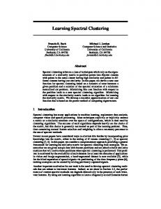
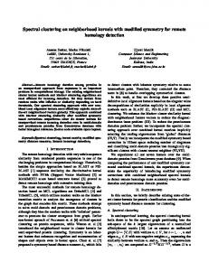
1. Introduction 1.1. Preface The objective of cluster analysis is to divide a given set of data into subsets, such that those subsets represent a certain similarity of the data itself. For example, let us look at the data points shown on the left picture in Figure 1. The human eye instantly recognizes two geometric shapes, two half-moons, and is able to divide the data into two clusters, where points within the same cluster belong to the same half-moon. However, in general, and especially with data from real world problems, it is not possible to just look at the data, so we need to rely on algorithms to do this. Conventional cluster analysis has various kinds of algorithms, one of the most popular being the k-means algorithm. It is fairly easy to understand and often gives satisfying results, but k-means also has many disadvantages. For example, it would fail to cluster the example shown in Figure 1, since it relies only on the pairwise distances between points and fails to detect patterns. This is where spectral clustering comes into play. In spectral clustering methods, we try to transform the given data in a manner, such that conventional algorithms like k-means can easily detect the correct patterns. In order to do that, we utilize eigenvalues and eigenvectors, thus explaining the name spectral clustering. Spectral clustering has become especially popular because it is fairly easy to implement, using only basic linear algebra, and gives fast and accurate results, even for more general sets of data. On the right picture in Figure 1, we can see the resulting clusters calculated by using a spectral clustering algorithm. We can agree that this result matches our intuitive expectations quite well, however, much is yet unknown about why spectral algorithms work as well as they do. In this thesis, mainly based on the work of [Luxburg07], we want to introduce the reader to the basics of spectral clustering and develop an implementation of the presented algorithms. In Section 2, we are going to introduce basic concepts needed for our later work and the terminology behind it. After recalling the meaning of eigenvalue problems, we will take a look at a fairly simple, but effective, clustering algorithms that we will be using to ultimately cluster our data after applying spectral methods. We will then focus on an introduction to graph theory,
6
1.1. Preface
Clustered Data
Data 0.6
0.6
0.4
0.4
0.2
0.2
0
0
−0.2
−0.2
−0.4
−0.4
−0.6
−0.6
−0.8 −0.8
−0.6
−0.4
−0.2
0
0.2
0.4
(a) Unclustered Data
0.6
0.8
−0.8 −0.8
−0.6
−0.4
−0.2
0
0.2
0.4
0.6
0.8
(b) Clustered Data
Figure 1: The first picture shows a sample set of data points in the shape of two half-moons. The second picture shows the clusters found by applying a spectral clustering algorithm.
discussing similarity graphs, describing the similarity of given data sets, graph Laplacians and graph cut problems, which will eventually lead us to the spectral methods being studied in this thesis. The main work will be seen in Section 3 where we will derive different spectral clustering algorithms by approximating the graph cut problems from the preceding section. Furthermore, we are going to discuss a few properties and problems of these methods, but also talk about their advantages and look at applications of spectral clustering. The next part, Section 4, is dedicated to the implementation of the algorithms we just got to know. We will be using MathWorks’ MATLAB as the programming language and platform to get the different algorithms to work and discuss advantages and disadvantages of this implementation. In the last section, we will put the MATLAB program we just developed to work, run it on different types of data sets and take a look at both the quality and the problems of spectral clustering. We will see typical behavior, advantages to more simple algorithms like k-means and boundaries to the abilities of spectral methods.
7
1. Introduction Acknowledgements Thanks to my stochastics professor and advisor for this thesis, Prof. Dr. Ingo Steinwart, for his inspirational and motivating way of teaching and for supervising me throughout the process of writing this thesis. A special thanks goes out to my friend Patricia Concepcion, who, despite being a mathematical layman, made the time for proofreading this work, therefore enabling me to write this thesis in English in the first place. Thanks to all my friends on www.matheboard.de for getting me interested in mathematics, helping me with any questions over the course of my studies and becoming like a second family to me. I apologize for not listing them individually since this would take too much space, and I would likely forget someone. Also thanks to my actual family, especially my parents, for supporting me in every way possible and without whom I would have never made it to the point of writing this.
8
1.2. Honesty Declaration
1.2. Honesty Declaration I hereby declare that the work submitted is my own and that all passages and ideas that are not mine have been fully and properly acknowledged. Furthermore, I declare that this work has not been in parts or wholly published as a submission for another examination procedure and that all copies, both printed and electronic, are the same.
08/09/2012 Date and Signature
9
2. Preparation and Terminology In this section we are going to introduce some concepts that we will be needing for our work on spectral clustering methods. We will take a quick look at eigenvalue problems and then proceed to discuss a basic, non-spectral clustering algorithm that we will use to cluster our data after applying spectral methods. The main part of this section, however, will be on graphs. We are going to introduce the general concept of graphs, talk about the similarity graphs describing the pairwise similarities between data points of a given set of data, define the Graph Laplacians and study some of their properties. Finally, we are going to introduce graph cut problems, representing the graph version of the clustering problem. Solving those graph cut problems, using approximations, will lead us to the spectral algorithms that we are looking for.
2.1. Eigenvalues and Eigenvectors Eigenvalue problems play a major role in several fields of mathematics, but since it is not the objective of this work to introduce to eigenvalues and eigenvectors, we are going to keep the section on them fairly short. Furthermore, we are going to focus on real-valued situations rather than arbitrary vector spaces. Definition 1: Let n ∈ N and A ∈ Rn×n be a real-valued, square matrix. If there is a vector x ∈ Rn×1 \ {0} such that Ax = λ x for some λ ∈ R, we call v an eigenvector to the eigenvalue λ . It can be shown that symmetric matrices have at least one eigenvalue, which is of interest to us since we will be looking at such matrices later on. A relatively straight-forward approach to calculating eigenvalues is looking for zeros of the characteristic polynomial det(A − λ I), where I is the n-by-n identity matrix. Eigenvectors to a certain eigenvalue λ can then be found by solving the linear equation system (A − λ I)x = 0. For large matrices this can be quite expensive work. We will face large matrices containing mostly zeros for several reasons that will be explained when talking about similarity graphs. Such sparse structured matrices can be handled more efficiently by using, for example, the Lanczos algorithm. There
11
2. Preparation and Terminology exist several variations of this algorithm in order to improve the numerical stability. We will not discuss this very complex topic any further here and rather reference to [Golub96] and [Saad11].
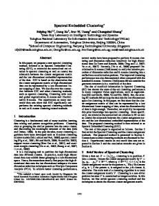
2.2. Basic Clustering Algorithms 2.2.1. k-Means Algorithm There exist many algorithms for cluster analysis, each one having its own benefits and disadvantages. A very common and often-used method is the kmeans algorithm. The idea behind this particular algorithm is rather intuitive, and though it’s very simple, k-means is still an extremely fast algorithm which is one of its biggest advantages. On the other hand, this algorithm is very limited and often doesn’t result in good clustering. It can be shown that finding an optimal clustering with k-means is actually a NP-hard problem1 . In our later work we are, in a way, going to transform the given data such that the classic k-means algorithm will be able to easily cluster the data, thus giving us a much better result than just running k-means. For those reasons, we will now discuss the classic k-means algorithm. k-means is an iterative algorithm that refines the result in every iteration. Before starting the algorithm, one has to choose a number k of clusters to look for. The standard k-means algorithm then consists of the following steps that are being visualized in Figure 2: 1. 2. 3. 4.
Randomly choose k cluster centroids. Assign each datum to the cluster with the closest centroid. Recalculate the centroids for each cluster. Go back to Step 2 until the algorithm terminates.
With this brief description, there are several questions to answer. First of all, since this is an iterative algorithm, we need a suitable exit condition. Usually, we would either set a maximum number of iterations, abort when the new centroids do not differ from the old ones (or at least not too much) or a combination of both. Furthermore, assigning the data points to clusters based on the distance to the centroids, we obviously need a distance function for the 1 See [Mahajan09].
12
2.2. Basic Clustering Algorithms
(a) Choosing initial centroids
(b) Assigning data points to clusters
(c) Updating centroid positions
(d) Refining cluster assignments
Figure 2: Visualization of k-means algorithm.
data. Usually, we would use the Euclidean metric or similar known metrics, although the question of which metric to use depends on the particular data set. Consider, for example, the case of a 500-by-500 pixels picture. We store each pixel as a data point by using the horizontal and vertical position and the RGB channel values, ranging from 0.0 to 1.0, as attributes, giving us a fivedimensional data set. Using an unmodified Euclidean metric would not be a good idea because the pixel position has a much larger range than the color values. This would result in the position of the pixel having a much greater effect on the distance than the color, which in terms of segmenting the picture into areas of the same color will lead to bad results.
13
2. Preparation and Terminology Choosing the initial centroids is a critical step in k-means that can have a huge effect on the result. Therefore, choosing them randomly as mentioned above would not seem like the best idea. Indeed, there exists a variety of variations and improvements to the standard algorithm, in particular k-means++ tries to solve exactly this problem by choosing better initial centroids.
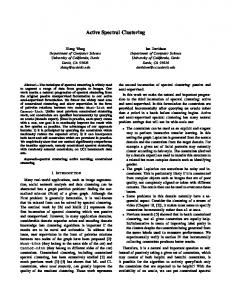
2.3. Graphs Next, we are going to introduce the general concept of graphs and then discuss the special kind of graph we will be needing. Then we will talk about graph Laplacians and graph cut problems that will lead us to the spectral clustering algorithms later on. 2.3.1. Notation Definition 2 (Graph): Let G = (V, E) with a non-empty and finite set V = {v1 , . . . , vn } of vertices and a set E ⊂ V × V of edges between such vertices. Then G is called a (directed) graph. If (vi , v j ) ∈ E, we denote this edge by ei j . Moreover, if E is symmetric, that is ei j ∈ E ⇔ e ji ∈ E for all edges, we call G an undirected graph. The similarity or distance of vertices in a graph could just be described by them being connected by an edge or not. However, this does not really allow for a deep level of information and we would much rather be able to describe these crucial information more freely. This is where the concept of weighted graphs comes into play. Definition 3 (Weighted Graph): Let G0 = (V, E 0 ) be a graph as defined above. 0 We now replace E 0 by E := E 0 × R+ 0 , which lets each edge ei j ∈ E carry a certain value wi j ≥ 0. Then, G := (V, E) is called a weighted graph and wi j is called the weight of the edge connecting vi and v j . Examples for the different types of graphs can be seen in Figure 3. Furthermore, from now on we will only consider undirected graphs. Our next step is to describe graphs with matrices the we will use to study their properties. Definition 4 (Adjacency Matrix): Let G = (V, E) be an undirected graph with weights wi j . If (vi , v j ) ∈ / E, we define wi j := 0. Then the matrix W = (wi j )i, j=1,...,n is called adjacency matrix of G.
14
2.3. Graphs
v2
v5
v2
v5
v3
v1
v1
v3
v4
v4
(a) Directed, unweighted
(b) Undirected, unweighted
v2 2
v5
3
v1 1
5
v3 10
v4 (c) Undirected, weighted
Figure 3: Different types of graphs with V = {v1 , . . . , v5 }.
15
2. Preparation and Terminology Since we were looking at an undirected graph, we have wi j = w ji for all weights which shows that W is symmetrical. Definition 5 (Degree Matrix): Let G be an undirected, weighted graph as above. Then di := ∑nj=1 wi j for some i ∈ {1, . . . , n} is called the degree of the vertex vi ∈ V . Furthermore, D = diag{d1 , . . . , dn } is called the degree matrix of G. Additionally, we will shorten {i | vi ∈ A} for a subset A ⊂ V by i ∈ A and then define W (A, B) :=
∑
wi j
i∈A, j∈B
for two arbitrary sets A, B ⊂ V . Later on, we will be forced to measure the size of a subset A ⊂ V . One way is to simply use the number of vertices in A, which is given by |A|. Another way, however, is to sum over the weights of edges attached to vertices in A, i. e. vol(A) := ∑i∈A di . If we think of graphs that contain components, which are not connected by edges, it makes sense that they will describe clusters we would like to find. In general, we cannot expect the graphs we are going to look at to be exactly structured like that. However, the structure will be similar to this situation. In order to study this in detail, we need to define what exactly we mean by components and their connections. Definition 6 (Connected Components): Let G be a graph as described above and A ⊂ V . We say that A is connected if there exists a path between any two vertices in A that lies completely in A, i. e. all points of this path are in A, too. Furthermore, we call A a connected component if it is connected and there is no connection between A and its complement Ac := V \ A. Definition 7 (Indicator Vector): Let A ⊂ V for a graph as described above. We then define the indicator vector of A by 1A = ( f1 , . . . , fn )0 ∈ Rn with ( 1 if vi ∈ A fi = . 0 otherwise
16
2.3. Graphs 2.3.2. Similarity Graphs After introducing the general concept of graphs, we will now take a look at a special kind of graphs that describe the pairwise similarity of the points in a given dataset. Definition 8 (Similarity Graph): Let D = {x1 , . . . , xn } be a given set of data and assume that we have values si j describing the similarity of xi and x j for all those data. We then construct the graph G = (V, E) by using the data points as vertices and weighting each edge with the corresponding similarity, i. e. wi j := si j . Then, G is called the similarity graph of this dataset. There are two things we need to point out: First of all, we will refer to both the graph itself and its adjacency matrix as similarity graph. Secondly, since for n data points the similarity graph will be a n-by-n matrix and because n is usually a large number, we need to consider technological limits in computer memory. We will therefore alter the shape of such similarity graphs to bycome these obstacles. The goal of this section is to discuss different approaches on how such similarity graphs can be obtained. This leads us to the idea of trying to make the matrix sparse, which means that most entries should be zeros. This allows us to store the matrix more efficiently rather than storing n2 entries individually, e. g. MATLAB uses a procedure called Compressed Sparse Column2 (CSC) to achieve this. There are different ways to construct sparse similarity graphs, and we are now going to discuss the most common types. However, we note first that in many situations, we have distances rather than similarity values between data points. We need to be careful about this since great similarity values are the equivalent of small distances and vice versa. Full Similarity Graph The easiest way to construct a similarity graph is simply connecting all vertices vi and v j with si j 6= 0. Keeping in mind that the similarity graph should model 2 The idea is to have an array containing the non-zero values, another array containing the row indices for those values and a third array containing the indices of the value array where a new column starts.
17
2. Preparation and Terminology local neighborhoods, a standard approach for fully connected graphs would be a Gaussian similarity function � � d(xi , x j )2 , si j := exp − 2σ 2 where σ is a parameter controlling the size of these neighborhoods. The metric d could, for example, be the Euclidean metric. The obvious disadvantage to this type of similarity graphs is that it lacks the sparse structure we desire. This is why this graph type is not recommended for large data sets. k-Nearest Neighbors Similarity Graph A better approach in terms of memory efficiency is the k-nearest neighbors graph type. We connect vi with v j , if v j is among the k nearest neighbors of vi , where k is a fixed number. The simple example in Figure 4, however, shows that this usually results in a directed graph. To convert it into an undirected similarity graph, we can use either one of the following two methods: • Normal k-Nearest Neighbors: We connect the vertices if either one of them is among the k-nearest neighbors of the other one. • Mutual k-Nearest Neighbors: We connect the vertices if vi is among the k-nearest neighbors of v j and v j is among the k-nearest neighbors of vi . For both types we use the similarity3 of vi and v j to weight the edge. Figure 5 shows two k-nearest similarity graphs. v1
v2
v3
Figure 4: The nearest neighbor of v3 is v2 , but the nearest neighbor for v2 is v1 , therefore the 1-nearest neighbor graph would be directed.
3 We can obtain similarity values from distances by applying a similarity function to only the connected vertices.
18
2.3. Graphs
Similarity Graph
Similarity Graph
1.5
1.2
1
0.8
1
0.6 0.5
0.4 0.2
0
0 −0.2
−0.5
−0.4 −0.6
−1 −1.5
−1
−0.5
0
0.5
1
1.5
2
2.5
−0.8 −1.5
(a) One connected component
−1
−0.5
0
0.5
1
1.5
2
2.5
(b) Two connected components
Figure 5: Both pictures show a k-nearest neighbor similarity graph for the situation of two half-moons as seen in Figure 1. In the case of two connected components, the components represent a desirable clustering result. We will further study this behavior later on.
ε-Neighborhood Similarity Graph The last type we look at is the ε-neighborhood graph type. Here, we simply connect vi and v j if d(xi , x j ) < ε for a fixed threshold ε > 0. Because the distances between connected points are numerically similar and at most ε, we consider this graph to be unweighted. 2.3.3. Graph Laplacians Graph Laplacians are matrices representing graphs in a certain way. Spectral graph theory is the study of these matrices because they turn out to be holding many useful information about the graphs. We will study some of these properties in this section so that we can use them later on for our spectral algorithms. As before, G is assumed to be an undirected and weighted graph with adjacency matrix W and degree matrix D. Definition 9: The unnormalized graph Laplacian is defined as L = D −W .
19
2. Preparation and Terminology As mentioned above, despite its simple structure, graph Laplacians have very interesting properties: Proposition 1: Let L be a graph Laplacian as defined above. Then we have the following properties: 1. For every vector ( f1 , . . . , fn )0 = f ∈ Rn we have f 0L f =
1 n wi j ( fi − f j )2 . 2 i,∑ j=1
2. L is symmetric and positive semi-definite. 3. The smallest eigenvalue of L is 0, a corresponding eigenvector is the constant one vector 1. 4. L has n non-negative, real-values eigenvalues 0 = λ1 ≤ λ2 ≤ . . . ≤ λn . Proof. Let us take a look at the statements individually: 1. Using the definition of L and the degrees di , we get f 0 L f = f 0 (D −W ) f = f 0 D f − f 0W f n
n
= ∑ di fi2 − i=1
1 = 2 1 = 2
∑
fi f j wi j
i, j=1
n
∑
n
di fi2 − 2
i=1
∑
i, j=1
n
∑
i, j=1 n
fi f j wi j + ∑
d j f j2
j=1
∑
!
n
n
wi j fi2 − 2
!
n
fi f j wi j +
i, j=1
=
� 1 wi j fi2 − 2 fi f j + f j2 ∑ 2 i, j=1
=
1 n wi j ( fi − f j )2 . 2 i,∑ j=1
∑
wi j f j2
i, j=1
In particular, as a sum over non-negative numbers, this shows f 0 L f ≥ 0 for all f ∈ Rn . 2. W is symmetric because we assume the graph to be undirected. The degree matrix D is obviously symmetric too, therefore L is symmetric.
20
2.3. Graphs The positive semi-definiteness follows from f 0 L f ≥ 0 for all f ∈ Rn , which we have just seen. 3. We want to verify that L1 = 0. By definition of the graph Laplacian, this is equivalent to D1 = W 1. Both D1 and W 1 are n-by-1 vectors containing the row sums of D respectively W . The sum of the i-th row of W is exactly what we defined to be di , which in turn is also the sum of the i-th row of D because D is a diagonal matrix. This shows that both vectors are the same, thus proving L1 = 0. 4. We have shown that L is symmetric and positive-definite. Therefore, all eigenvalues are real-valued and non-negative. An important property for spectral clustering in particular is the following result. Proposition 2: Let G be an undirected, weighted graph. Then the geometric multiplicity k of the eigenvalue 0 of L equals the number of connected components in the graph. The eigenspace of this eigenvalue is spanned by the indicator vectors of those components. Proof. We start by looking at the case of a connected graph, that is k = 1, and then reduce the general case to this one. Let f be an eigenvector with eigenvalue 0, that is L f = 0 and therefore f 0 L f = f 0 0 = 0, then according to Proposition 1 we have 0 = f 0L f =
1 n wi j ( fi − f j )2 . 2 i,∑ j=1
As already mentioned in the proof of the first property in Proposition 1, the sum can only equal zero if all terms wi j ( fi − f j )2 vanish. Since we have wi j > 0 for two connected vertices vi and v j , we can conclude fi = f j . Therefore, f needs to be constant for all vertices in the graph that can be connected and since we assumed the graph to be connected, f has to be constant on the whole graph. Of course, every multiple of an eigenvector is an eigenvector, but since we usually treat them as one, we see that f = 1 is the only eigenvector with eigenvalue 0. It is obvious that this is the indicator vector for the connected component. Now we are going to look at arbitrary k, that is we have k connected components. Obviously, we can change the order of the vertices without changing
21
2. Preparation and Terminology the graph and therefore sorting them by the connected components they belong to, we can achieve that the adjacency matrix W has a block diagonal form. Then, we also get such a form for L1 0 . . . 0 .. 0 L2 . . L= .. .. . . 0 0 . . . 0 Lk Each one of these blocks Li is a graph Laplacian on its own and therefore represents a graph. More precisely, it represents the i-th connected component subgraph of G. Since L is in block diagonal form, its spectrum equals the union of the spectra of Li and we get the corresponding eigenvectors by filling all other entries with zeros. The first step has shown that each Li has the constant vector 1 as an eigenvector with eigenvalue 0. Therefore, the number of eigenvalues 0 of L equals the number of connected components and the corresponding eigenvectors are exactly their indicator vectors. The graph Laplacian we got to know so far is often referred to as the unnormalized graph Laplacian, suggesting that it can be normalized in some sense. In fact, there are many different ways to normalize it, but they usually don’t have names on their own and are just referred to as the normalized graph Laplacian. We are going to introduce two different ways to normalized the graph Laplacian, leading to two different spectral clustering algorithms later on. Definition 10: We define the two normalized graph Laplacians 1
1
Lsym := D− 2 LD− 2 and Lrw := D−1 L. Note that in order for these matrices to be well-defined, we need det D = ∏i di 6= 0, otherwise the inverse matrix would not exist. This is equivalent to di 6= 0 for all i. We can safely assume wii > 0 for all i and recalling the definition of the degrees, we get di ≥ wii > 0. We chose those names for the normalized graph Laplacians, as Lsym is a symmetric matrix and Lrw is related to a random walk. As before, we are going to take a look at a few important properties of both graph Laplacians.
22
2.3. Graphs Proposition 3: Let Lsym and Lrw be defined as above, then we have the following properties: 1. For every vector ( f1 , . . . , fn )0 = f ∈ Rn we have 1 n f Lsym f = ∑ wi j 2 i, j=1 0
fj f √i − p di dj
!2 .
2. λ is an eigenvalue of Lrw with eigenvector u if and only if λ is an eigen1 value of Lsym with eigenvector w = D 2 u. 3. λ is an eigenvalue of Lrw with eigenvector u if and only if λ and u solve the generalized eigenproblem Lu = λ Du. 4. 0 is an eigenvalue of Lrw with the constant one vector 1 as eigenvector. 0 1 is an eigenvalue of Lsym with eigenvector D 2 1. 5. Lsym and Lrw are positive semi-definite and have n non-negative, realvalued eigenvalues 0 = λ1 ≤ . . . ≤ λn . Proof. Once again, we look at the statements individually: 1
1. The matrix D− 2 is a diagonal matrix containing 1 f 0 D− 2
1 D− 2
√1 di
on the i-th diagonal
element. Therefore, and f are just scaled versions of the vectors f 0 and f , where each entry fi has been replaced with √fdi . i Substituting these vectors with g0 and g, we have the same situation as in Proposition 1. 2. Let w be an eigenvector of Lsym to the eigenvalue λ , that is Lsym w = λ w. 1 1 1 Multiplying with D− 2 from the left gives us D− 2 Lsym w = D− 2 λ w. With 1
1
1
1
1
1
D− 2 Lsym = D− 2 D− 2 LD− 2 = D−1 LD− 2 = Lrw D− 2 , 1
1
1
this leads us to Lrw D− 2 w = λ D− 2 w and substituting u = D− 2 w gives us the eigenvalue equation Lrw u = λ u for Lrw . 3. Starting with Lrw u = λ u, we multiply D onto both sides from the left and with DLrw = DD−1 L = L, we get Lu = λ Du.
23
2. Preparation and Terminology 4. From Proposition 1 we know that L1 = 0. Therefore, we get Lrw 1 = D−1 L1 = D−1 0 = 0, i. e. 1 is an eigenvector to eigenvalue 0. The other statement is a direct consequence of 2. 5. Just like in Proposition 1, the statement about Lsym follows from 1 and then 2 shows it for Lrw . As before with the unnormalized graph Laplacian, we can derive a similar result as in 2 for normalized graph Laplacians. Proposition 4: Let G be an undirected, weighted graph. Then the geometric multiplicity k of the eigenvalue 0 of both Lsym and Lrw equals the number of connected components A1 , . . . , Ak in the graph. For Lrw , the eigenspace of 0 is spanned by the indicator vectors 1Ai of those 1 components. For Lsym , the eigenspace of 0 is spanned by the vectors D 2 1Ai . Proof. We can prove this proposition just like Proposition 2 by using the properties from Proposition 3. 2.3.4. Graph Cuts Up to this point we developed some solid theory about graphs and their spectral properties. However, originally we wanted to solve a clustering problem. Representing the data with a graph like we discussed it before, we are now able to rephrase the clustering problem and express it in the language of graphs. That is, we are looking for a partition4 of the graph such that each group represents a collection of data points with high weights to each other while points from different groups have very low weights. Spectral clustering algorithms will then be the result of approximating this problem. Definition 11: Let W be the adjacency matrix of a given similarity graph and k ∈ N. Then, minimizing cut(A1 , . . . , Ak ) :=
1 k ∑ W (Ai , Aci ) 2 i=1
for A1 , . . . , Ak ⊂ V is called the mincut problem. 4 A partition is a set of non-empty, disjoint subgraphs such that their union equals the whole graph.
24
2.3. Graphs However, solving the mincut problem often leads to separating a single vertex from the rest of the graph, which of course is not what we would like to see when clustering data. Therefore, we want to work in the condition of the sets A1 , . . . , Ak being large in some sense. In a previous section, we already introduced two ways to measure the size of such sets. This leads to the following graph cut problems: Definition 12: Given the adjacency matrix W as above, the RatioCut problem consists of minimizing RatioCut(A1 , . . . , Ak ) :=
k cut (Ai , Aci ) 1 k W (Ai , Aci ) =∑ . ∑ |Ai | |Ai | 2 i=1 i=1
Definition 13: Given the adjacency matrix W as above, the Ncut problem (short for normalized cut) consists of minimizing Ncut(A1 , . . . , Ak ) :=
k cut (Ai , Aci ) 1 k W (Ai , Aci ) =∑ . ∑ 2 i=1 vol(Ai ) i=1 vol(Ai )
Both cut problems try to balance the size of the groups Ai , but they are trying to achieve this in different ways: The RatioCut problem takes the number of vertices in each group into account, while the Ncut problem uses the edge weights for this. While solving these problems would give us better results, the downside is that, unlike the original mincut problem, which is easy to solve, they are hard to solve. In fact, it can be shown that they are NP-hard5 . Therefore, instead of solving it exactly, we will rely on approximating the solutions. This will finally lead us to the spectral clustering algorithms.
5 See [Wagner93].
25
3. Spectral Clustering We now have all the tools we need to get started on deriving spectral clustering algorithms. In order to do so, we will approximate the graph cut problems we discussed in the previous section. These approximations are done by a relaxation step, where we switch from a discrete to a continuous problem. We will see that relaxing Ncut and RatioCut leads to different algorithms. We will also summarize the algorithm in a way so that it can be realized on computers since we will be doing that in the next section. Furthermore, we are going to talk about the complexity of spectral clustering algorithms and briefly discuss some of its applications.
3.1. Unnormalized Algorithm In order to make things easier to understand, we will start out with approximating RatioCut in the special case of two clusters. With the second step, we will transfer the idea of that scenario to the general case of arbitrary k. 3.1.1. Derivation for k = 2 We begin with approximating RatioCut for k = 2 and recall that the problem we want to solve is min RatioCut (A, Ac ) .
(1)
A⊂V
First, we introduce the vector f = ( f1 , . . . , fn )0 ∈ Rn that is defined by q c |A | for vi ∈ A q |A| fi = . − |A|c for vi ∈ Ac |A | Proposition 5: Let L be the graph Laplacian of a given graph, A ⊂ V and f as defined above. Then, we have f 0 L f = |V | · RatioCut(A, Ac ).
27
3. Spectral Clustering Proof. Using Proposition 1, we get 1 n wi j ( fi − f j )2 2 i,∑ j=1 s s !2 |Ac | |A| 1 = wi j + |A| |Ac | 2 i∈A,∑ j∈Ac s s !2 |Ac | |A| 1 + wi j − − |A| |Ac | 2 i∈A∑ c , j∈A !� � |Ac | |A| 1 w + w + + 2 = i j i j ∑ |A| |Ac | 2 i∈A,∑ j∈Ac i∈Ac , j∈A � c � |A | |A| = cut(A, Ac ) + +2 |A| |Ac | � � |A| + |Ac | |A| + |Ac | c = cut(A, A ) + |A| |Ac |
f 0L f =
= |V | · RatioCut(A, Ac ). Proposition 6: Let f be defined as above, then 1. f ⊥1 and 2. k f k2 = n. Proof. Simply computing the inner product, we get s s s s n |Ac | |A| |Ac | |A| f 1 = ∑ fi = ∑ −∑ = |A| − |Ac | c| c| |A| |A |A| |A i=1 i∈A i∈Ac = 0, therefore we have f ⊥1. Furthermore, we have n
k f k2 = ∑ fi2 = |A| i=1
28
|Ac | |A| + |Ac | c = |A| + |Ac | = n. |A| |A |
3.1. Unnormalized Algorithm Combining Proposition 5 and Proposition 6, we can rewrite the problem in (1) as ( f defined as above and f ⊥1 0 . (2) min f L f with √ A⊂V kfk = n Since we haven’t actually used any kind of relaxation or approximation so far, but rather just changed the point of view, the problem, of course, is still NP-hard. We are now going to allow the entries of f to take arbitrary values rather than just two particular values, therefore getting rid of the discreteness of the problem. By doing so, we finally get a relaxed version of the problem: ( f ⊥1 0 min f L f with . (3) √ f ∈Rn kfk = n To solve the problem given in (3), we will take a look at the Rayleigh-Ritz Theorem, which, in combination with a more general version of it, will tell us the solution. Theorem 1 (Rayleigh-Ritz 1): Let A ∈ Rm×m be a symmetric matrix, then the smallest and largest eigenvalues are given by � 0 � x Ax m λmin (A) = min | 0 = 6 x ∈ R x0 x respectively � x0 Ax m λmax (A) = max | 0 6= x ∈ R . x0 x �
Proof. See [Horn85]. Ignoring the additional conditions, the solution of (3), according to Theorem 1, would be given by the eigenvector corresponding to the smallest eigenvalue. However, from Proposition 1 we know that this is the constant one vector 1, which obviously cannot solve (3) because it violates the condition f ⊥1. Proposition 7: The solution of (3) is given by the eigenvector to the second smallest eigenvalue of L.
29
3. Spectral Clustering Proof. Proposition 1 showed that L is symmetric, therefore √we can consider the spectral decomposition of L and find n eigenvectors 1 n = v1 , v2 , . . . , vn √ which are orthogonal to each other and have norm n. This guarantees vi ⊥1 √ and kvi k = n for all i ∈ {2, . . . , n}, in other words all of these eigenvectors but v1 meet the conditions in (3). This shows that the solution of (3) is given by some eigenvector of L. A generalized version of the Rayleigh-Ritz Theorem now shows that it is, in fact, the eigenvector corresponding to the second smallest eigenvalue of L. The next step is to undo the relaxation and go back from real values to a discrete indicator vector. In order to do this, we consider the coordinates fi to be points in R and use the 2-means algorithm to obtain two clusters C and Cc . We can then use this clustering by setting ( vi ∈ A if fi ∈ C . vi ∈ Ac if fi ∈ Cc 3.1.2. Derivation for Arbitrary k Now that we discussed the special case k = 2, we go on to studying the case of arbitrary k ∈ N. The general idea is the same, but we will have to make a few technical changes. For a given partition A1 , . . . , Ak ⊂ V we define the indicator vectors h j = (h1, j , . . . , hn, j )0 by q1 if vi ∈ A j |A j | hi j = 0 if vi ∈ / Aj for all i ∈ {1, . . . , n} and j ∈ {1, . . . , k} and define H ∈ Rn×k to be the matrix containing those vectors as columns. Proposition 8: With the notation given as above, we have 1. h0i Lhi =
cut(Ai , Aci ) and |Ai |
2. h0i Lhi = (H 0 LH)ii . Proof. The proof is similar to the proof of Proposition 5.
30
3.1. Unnormalized Algorithm Proposition 9: Let tr(A) denote the trace of a matrix A, that is the sum of the entries on its diagonal. Then we have RatioCut(A1 , . . . , Ak ) = tr(H 0 LH). Proof. Using Proposition 8 twice, we get k
k
i=1
i=1
RatioCut(A1 , . . . , Ak ) = ∑ h0i Lhi = ∑ (H 0 LH)ii = tr(H 0 LH). Proposition 8 and Proposition 9 allow us to rewrite the RatioCut problem to ( H as defined above 0 min tr(H LH) with , (4) A1 ,...,Ak H 0H = I wherein we see H 0 H = I because the columns of H are orthonormal. Allowing the entries of H to take arbitrary values relaxes the problem in a similar way as we have done it for k = 2. This leads us to the relaxed RatioCut problem min tr(H 0 LH) with H 0 H = I.
(5)
H∈Rn×k
At this point, we will introduce another version of the Rayleigh-Ritz Theorem, which, similarly to the special case of k = 2, will help us to find the solution of (5). Theorem 2 (Rayleigh-Ritz 2): Let A ∈ Rm×m be a symmetric matrix with eigenvalues λ1 ≤ . . . ≤ λm and let v1 , . . . , vm be the corresponding orthonormal eigenvectors. Then the solution of the optimization problem min tr(X 0 AX) with X 0 X = I
X∈Rm×n
for some n ∈ {1, . . . , m} is given by the matrix X containing the first n eigenvectors as columns. Proof. See [Horn85]. We can now retrieve a solution for (5) from Theorem 2 and see that it is given by the matrix H containing the first k eigenvectors6 as columns. And also, just like before, using k-means on the rows of H to transform the real-valued problem to a discrete problem will give us the clustering. 6 Here and anytime else we refer to the first k eigenvectors as the eigenvectors corresponding to the k smallest eigenvalues.
31
3. Spectral Clustering 3.1.3. The Algorithm The algorithm we just presented used the unnormalized graph Laplacian L, which is why we refer to this algorithm as the unnormalized spectral clustering algorithm. In simple words, the algorithm is given as in Figure 6. Let S ∈ Rn×n be the similarity matrix for the n points x1 , . . . , xn , where si j describes the similarity between xi and x j . Let k be the desired number of clusters. 1. Construct a similarity graph with adjacency matrix W as discussed before. 2. Compute the unnormalized graph Laplacian L = D −W . 3. Compute the first k eigenvectors u1 , . . . , uk of L. 4. Let U ∈ Rn×k be the matrix containing the vectors u1 , . . . , uk as columns. 5. For i = 1, . . . , n let yi ∈ Rk be the vector corresponding to the i-th row of U. 6. Cluster the points (yi )ni=1 into clusters C1 , . . . ,Ck using the k-means algorithm. 7. Retrieve clusters A1 , . . . , Ak by Ai = { j | y j ∈ Ci }. Figure 6: Unnormalized spectral clustering.
3.2. Normalized Algorithms We have seen that approximating RatioCut leads to an algorithm using the unnormalized graph Laplacian. Similarly, we will now approximate the Ncut problem and we are going to see that this leads to an algorithm involving normalized graph Laplacians.
32
3.2. Normalized Algorithms 3.2.1. Derivation for k = 2 Again, we start out by looking at the special case of k = 2. We define the cluster indicator vector by q vol(Ac ) if vi ∈ A vol(A) q . fi = − vol(A)c if vi ∈ Ac vol(A ) Proposition 10: Let f be the cluster indicator vector as defined above. Then, we have 1. (D f )0 1 = 0 and 2. f 0 D f = vol(V ). Proof. Both equations are shown by simple calculations. We have n
(D f )0 1 = ∑ di fi i=1
s
s vol(Ac ) vol(A) −∑ = ∑ di vol(A) i∈Ac vol(Ac ) i∈A s s vol(Ac ) vol(A) = ∑ di − vol(Ac ) ∑c di vol(A) i∈A i∈A s s vol(Ac ) vol(A) = vol(A) − vol(Ac ) vol(A) vol(Ac ) p p = vol(Ac ) vol(A) − vol(A) vol(Ac ) = 0, proving the first statement. For the second equation, we have n
f 0 D f = ∑ fi2 di i=1
vol(Ac ) vol(A) di + ∑ d c) i vol(A) vol(A i∈A i∈Ac
=∑
= vol(Ac ) + vol(A) = vol(V ).
33
3. Spectral Clustering Proposition 11: In the situation as described above, we have f 0 L f = vol(V ) Ncut(A, Ac ). Proof. Utilizing Proposition 1 we can see that 1 n wi j ( fi − f j )2 2 i,∑ j=1 s s !2 1 vol(Ac ) vol(A) = wi j + 2 i∈A,∑ vol(A) vol(Ac ) j∈Ac s s !2 vol(A) vol(Ac ) 1 wi j − − + 2 i∈A∑ vol(Ac ) vol(A) c , j∈A !� � 1 vol(Ac ) vol(A) = wi j + ∑ wi j + +2 2 i∈A,∑ vol(A) vol(Ac ) j∈Ac i∈Ac , j∈A � � vol(Ac ) vol(A) + + 2 = cut(A, Ac ) vol(A) vol(Ac ) � � vol(Ac ) + vol(A) vol(A) + vol(Ac ) = cut(A, Ac ) + vol(A) vol(Ac )
f 0L f =
= vol(V ) Ncut(A, Ac ). Combining Proposition 10 and Proposition 11, we can rewrite the problem as ( f as defined above and D f ⊥1 0 min f L f with . (6) A f 0 D f = vol(V ) As we did it several times by now, we allow f to take arbitrary values, thus relaxing the problem to ( D f ⊥1 0 . (7) minn f L f with f ∈R f 0 D f = vol(V )
34
3.2. Normalized Algorithms 1
A step that is new to us is to substitute g := D 2 f , which transforms the problem to ( 1 1 1 g⊥D 2 1 0 −2 −2 min g D LD g with . (8) g∈Rn kgk2 = vol(V ) 1
1
We can now see that D− 2 LD− 2 = Lsym , whose first eigenvector, according 1 to Proposition 3, is D 2 1. Since vol(V ) is a constant, we can once again use the Rayleigh-Ritz Theorem to see that the solution g of (8) is given by the second eigenvector of Lsym . By using Proposition 3, we can furthermore see 1 that f = D− 2 g is the second eigenvector of Lrw . From here on, the rest is just like in the case of the unnormalized spectral algorithm: We cluster the coordinates fi ∈ R using the 2-means algorithm in order to restore the discreteness and obtain the clusters. 3.2.2. Derivation for Arbitrary k After taking a look at k = 2, we are now going to relax the Ncut problem for an arbitrary number of clusters. We define the indicator vectors h j = (h1, j , . . . , hn, j )0 by hi, j =
1 vol(A j )
√
if vi ∈ A j
0
if vi ∈ / Aj
(
for all i ∈ {1, . . . , n} and j ∈ {1, . . . , k} and once again set H to be the matrix containing these indicator vectors as columns. Proposition 12: In the described situation, we have 1. H 0 H = I, 2. h0i Dhi = 1 and 3. h0i Lhi =
cut(Ai , Aci ) . vol(Ai )
Proof. All equations can be proven by calculations that are similar to the ones before.
35
3. Spectral Clustering With Proposition 12, we now rewrite the Ncut problem as ( H as defined above 0 min tr(H LH) with A1 ,...,Ak H 0 DH = I
.
(9)
and relax the problem by allowing H to take arbitrary values, but also substi1 tute T = D 2 H, thus giving us � � 1 1 (10) min tr T 0 D− 2 LD− 2 T with T 0 T = I. T ∈Rn×k
Again, we can see that the solution T is given by the matrix containing the 1 first k eigenvectors of Lsym as columns and resubstituting H = D− 2 T shows that H is given by the matrix containing the first k eigenvectors of Lrw as columns. Of course, we now run k-means on the rows of H again to get discrete indicator vectors and obtain the clusters. 3.2.3. The Algorithms Relaxing Ncut as we did above leads to an algorithm using the eigenvectors of Lrw . Therefore, we call this a normalized spectral clustering algorithm that is given as shown in Figure 7. Figure 8 shows a different version of the normalized spectral clustering algorithm, which uses eigenvectors of Lsym rather than Lrw . However, we need to introduce an additional step in which we normalize the rows of the matrix U that contains the eigenvectors as columns. This step can be explained using perturbation theory, i. e. looking at the difference between the ideal case and real scenarios. However, this is beyond the scope of this thesis and will therefore not be explained. For a short discussion on this, we refer to [Luxburg07, Section 7.2].
36
3.2. Normalized Algorithms
Let S ∈ Rn×n be the similarity matrix for the n points x1 , . . . , xn , where si j describes the similarity between xi and x j . Let k be the desired number of clusters. 1. Construct a similarity graph with adjacency matrix W as discussed before. 2. Compute the unnormalized graph Laplacian L = D −W . 3. Compute the first k eigenvectors u1 , . . . , uk of the normalized graph Laplacian Lrw . 4. Let U ∈ Rn×k be the matrix containing the vectors u1 , . . . , uk as columns. 5. For i = 1, . . . , n let yi ∈ Rk be the vector corresponding to the i-th row of U. 6. Cluster the points (yi )ni=1 into clusters C1 , . . . ,Ck using the k-means algorithm. 7. Retrieve clusters A1 , . . . , Ak by Ai = { j | y j ∈ Ci }. Figure 7: Normalized spectral clustering according to Shi and Malik (2000).
37
3. Spectral Clustering
Let S ∈ Rn×n be the similarity matrix for the n points x1 , . . . , xn , where si j describes the similarity between xi and x j . Let k be the desired number of clusters. 1. Construct a similarity graph with adjacency matrix W as discussed before. 2. Compute the unnormalized graph Laplacian L = D −W . 3. Compute the first k eigenvectors u1 , . . . , uk of the normalized graph Laplacian Lsym . 4. Let U ∈ Rn×k be the matrix containing the vectors u1 , . . . , uk as columns. 5. Form the matrix T ∈ Rn×k from U by normalizing the rows, i. e. set ui j T = (ti j )ni, j=1 with ti j = � �1 . 2 ∑k u2jk 6. For i = 1, . . . , n let yi ∈ Rk be the vector corresponding to the i-th row of T . 7. Cluster the points (yi )ni=1 into clusters C1 , . . . ,Ck using the k-means algorithm. 8. Retrieve clusters A1 , . . . , Ak by Ai = { j | y j ∈ Ci }. Figure 8: Unnormalized spectral clustering according to Jordan and Weiss (2002).
38
3.3. Complexity
3.3. Complexity Cluster analysis is being used for a wide variety of applications and the size of the data sets may range from a few dozens or hundreds of data points to up to hundreds of thousands. For this reason, we would naturally be interested in some information on computational complexity of the algorithms. In order to do this, we will take a look at the computational complexity of individual steps of spectral clustering. As before, let n be the number of data points and d be their dimensionality. The very first step is constructing a similarity graph. Assuming that calculating a single similarity si j between two data points xi and x j involves at least one inner product, it costs us O(d) to calculate such a value. Therefore, constructing the whole graph has a time complexity of O(n2 d). Without going into too much detail, we can use a so-called max-heap7 to make it a k-nearest similarity graph. This requires us to restructure the heap constantly and results in an overall complexity of O(n2 log k) to make the already graph sparse. Next, we need to compute the eigenvectors corresponding to the smallest eigenvalues. This is a complex problem and many eigensolvers exist for this sort of task. As mentioned before, a common approach is the Lanczos algorithm8 and without going into details about how this algorithm works, we can derive a time complexity of O(m3 ) + (O(nm) + O(nt)) · O(p(m − k)), wherein m > k is the so-called Arnoldi length that is defined by the user and p is the number of restarted Arnoldi iterations. Just to give an idea about the values, m is usually set to be several times larger than k. For more precise information on how this complexity can be derived, we reference to [Song11]. The last step is running k-means on the eigenvector matrix. Within each iteration, we have to calculate the distances between any point and all the cluster centroids. This yields a time complexity of O(l · nk2 ), where l is the number of iterations for k-means. Overall, we can see that constructing the similarity graph is the most expensive step and considering that we usually want to work with large data sets, O(n2 ) 7 A max-heap is a tree-based data structure wherein the node with the greatest value is always the root node. See [Atkin86] for further information. 8 See [Saad11].
39
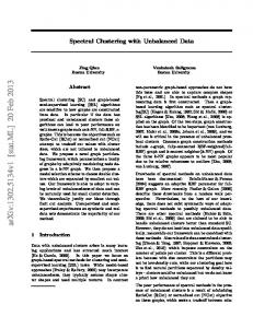
3. Spectral Clustering is a bottleneck. There exist several approaches to deal with this problem, for example by using parallel computing methods (see [Song11]) or relying on approximating algorithms (see [Yan09]). In Figure 9 we show the results of some experiments we ran using our MATLAB program. We created 50 data sets of three Gaussians, each consisting of n = 100, 1 · 200, . . . , 50 · 100 data points, and clustered them into three clusters using a 50-nearest similarity graph. We did this both for two- and threedimensional sets and plotted the computing time against n. We also calculated the average ratio when n is doubled and called this the Avg-value. If the algorithm has a complexity of O(n2 ), we would expect Avg ≈ 4 and indeed, our results match this expectation.
3.4. Comments Probably the most important comment to make on spectral clustering is to warn about its quality. While the methods are relatively efficient and seem to lead to satisfying results, it can be proven that there is no guarantee on them actually being accurate, i. e. the difference between RatioCut(A1 , . . . , Ak ) for the exact solution and RatioCut(B1 , . . . , Bk ) for the solution given by unnormalized spectral clustering can be arbitrarily large. In fact, this behavior can already be observed on relatively easy graphs9 . The reason for the popularity on spectral relaxation approaches is probably less the general quality of results, but rather the fact that it leads to simple problems from linear algebra that can be solved very easily. The next thing to talk about is not only a problem in spectral clustering, but also in many other clustering algorithms. In real-world data, we often do not know how many clusters we are looking for, but the algorithms require this number as an input. If we don’t have information about the data that enable us to give a good guess of this number, we are usually forced to run the algorithms with different parameters and compare the quality10 of the results. In spectral clustering, this is, in fact, not too bad of an approach since the most expensive step is constructing the similarity graph, but we don’t need the number of clusters for this step yet. Therefore, we can simply use the same graph over and over again, thus reducing computing time a lot. 9 See [Luxburg07, Section 5.4] for an example. 10 A few ways to do this are covered in the appendix and will be used in Section 5.
40
3.4. Comments
Time−Complexity of Spectral Clustering 40 Similarity Graph Clustering Algorithm Total t(n) = cn²
35
Time in seconds
30 25 20 15 10 5 0
0
5000 10000 Number of Data Points
15000
(a) 2-Dimensional, Avg = 3.50 Time−Complexity of Spectral Clustering 45 Similarity Graph Clustering Algorithm Total t(n) = cn²
40
Time in seconds
35 30 25 20 15 10 5 0
0
5000 10000 Number of Data Points
15000
(b) 3-Dimensional, Avg = 3.60
Figure 9: Computing time for spectral clustering plotted against the number n of data points.
41
3. Spectral Clustering Another approach would be to compute eigenvalues until we find the first k eigenvalues to be relatively small, while having a big eigengap |λk+1 − λk |. This can easily be justified or at least be made plausible by the theory about graph Laplacians discussed above, especially using Proposition 2. Constructing similarity graphs requires us to know other parameters such as a good number of nearest neighbors or the ε-parameter and their choice might be even more important than the number of clusters itself. There exist several approaches, which should usually be considered a "rule of thumb". A simple one of those is to choose the number k for the k-nearest similarity graph in logarithmic dependency of the number n of data points. More complex approaches use information that can be extracted from the data set very quickly. An example can be found in [Sugar03].
3.5. Applications Cluster analysis is used in a variety of situations, reaching into most sciences like physics, biology and medicine, and it is almost impossible to give a full list of applications. However, we want to take a brief look at some examples. In image segmentation we usually try to divide an image into certain segments or detect edges – a method useful, for example, both in image processing and medicine. Each pixel of a n-by-n pixels image represents a data point. Different attributes could be considered, for example the RGB values or the intensity. Therefore, we have n2 data points to work with, which would result in dealing with n2 -by-n2 matrices. Even for low-resolution images, this forces us to deal with very big datasets. A common approach to solve this problem is applying the clustering algorithms only to small blocks of the image and then merge the resulting segments with methods like a stochastic ensemble consensus. A detailed explanation can be found in [Tung10]. We will cover some examples of image segmentation in Section 5.3. Another possible application is in signal theory. Consider, for example, an audio file containing the voices of two persons talking at the same time. Then, we might want to separate this linear mixture of signals and filter out the individual voices. This yields a very complex problem, involving many more techniques besides cluster analysis. An in-depth discussion can be found in [Bach09].
42
3.5. Applications But the range of applications is even wider. We can use clustering results to predict certain attributes. Possible uses of this is predicting the age of animals based on physical attributes or detecting fake banknotes. Both examples will be covered in Section 5.2.
43
4. Programming 4.1. MATLAB In this section, we are going to show how to implement spectral clustering algorithms. We will be using MathWorks’ MATLAB since it is a powerful tool that allows us to manipulate and work with big matrices in an efficient and yet easy way. We will not go too deep into detail and discuss every possibility but rather focus on the main algorithm. For further information we advise the reader to look into the appended software that contains a lot of comments and documentation. Obviously, at this point, we assume that the reader has an understanding of how spectral clustering algorithms work. Before we start, we want to note a few things: • We assume to have a d-by-n matrix M containing m data points in d dimensions. We set n = size (M, 2); to be the number of data points. • Similarly to mathematical convention, but considering that i also stands for the imaginary unit in MATLAB, we denote loop counters with ii . • For a general improvement in computational efficiency, we will use column rather than row operations on matrices whenever possible. This increases speed due to the way MATLAB stores matrices in the memory. • We will use a routine called distEuclidean (M, N), giving us the Euclidean distances between the column-wise taken points of two d-by-n matrices. Furthermore, we use a function called simGaussian(M, sigma) that converts a distances matrix M into a similarity matrix by applying a Gaussian similarity function with parameter sigma, that is � � s(xi , x j ) = exp −
d(xi ,x j )2 2σ 2
.
4.1.1. Constructing Similarity Graphs The first thing we need to do is to construct a similarity graph W for the given set M of data points. We have discussed several ways on how to construct such a graph that we will now look at.
45
4. Programming Full Similarity Graph The first graph type is a full graph, which is the easiest one to construct. We need to calculate all pairwise distances and then apply a Gaussian similarity function with parameter σ , which can be done as shown in Listing 1. Listing 1: Creating a full similarity graph W = s q u a r e f o r m ( p d i s t (M ’ ) ) ; W = s i m G a u s s i a n (W, sigma ) ;
k-Nearest Similarity Graphs A little more work is required to construct a normal or mutual k-nearest similarity graph. Since the point to constructing such graphs is the sparse structure, we will use MATLAB’s sparse matrix routines. As recommended in the documentation, instead of creating and constantly modifying such a matrix, we rather store the indices and values of non-zero entries in vectors and then create the sparse matrix from them. For this, we first need to preallocate memory for those vectors as shown in Listing 2. Listing 2: Preallocating memory for sparse matrix vectors i n d i = zeros ( 1 , k * n ) ; i n d j = zeros ( 1 , k * n ) ; inds = zeros ( 1 , k * n ) ;
In order to find the k nearest neighbors, we need to loop through all data points, calculate the pairwise distances to all other data points and then sort them by their distance. We can then simply take the first k entries and create the sparse matrix. This is shown in Listing 3. Note that, in theory, we could get rid of this loop and since MATLAB is relatively slow with loops, this would seem like a good way to go. However, it would involve making MATLAB calculate a n-by-n matrix all at once, which will quickly take up too much memory. This, in return, will also make it slower because a standard computer would now use the hard-drive to store data that would be stored in the memory otherwise. Tests when writing this software have shown that even without reaching the memory limit, using a loop is actually faster in this case.
46
4.1. MATLAB Listing 3: Find k nearest neighbors for i i = 1 : n d i s t = d i s t E u c l i d e a n ( repmat (M( : , [ s , O] = s o r t ( d i s t , ’ a s c e n d ’ ) ;
i i ) , 1 , n ) , M) ;
i n d i ( 1 , ( i i −1) * k + 1 : i i * k ) = i i ; i n d j ( 1 , ( i i −1) * k + 1 : i i * k ) = O ( 1 : k ) ; i n d s ( 1 , ( i i −1) * k + 1 : i i * k ) = s ( 1 : k ) ; end W = sparse ( indi , indj , inds , n , n ) ;
However, the matrix W as constructed so far, will represent a directed graph. We can easily construct an undirected graph by doing the following: • For the normal k-nearest graph we execute W = max(W, W’);. • For the mutual k-nearest graph we execute W = min(W, W’);. The graph is currently only containing distances. We need to assign new values to the non-zero entries of W to convert it to a graph containing similarity values. We could just make the graph unweighted by using W = (W ~= 0); , but that is generally not a good idea because even few neighbors can be far away if the corresponding data point does not lie within a dense area of points. We rather call simGaussian(M, sigma), but have to be careful to only apply this to non-zero entries of W . The way this is done is shown in Listing 4. Listing 4: Applying Gaussian similarity function to non-zero entries of W W = spfun (@(W) ( s i m G a u s s i a n (W, sigma ) ) , W) ;
ε-Similarity Graph In case of an ε-graph, we have no idea whatsoever about how many data points will lie within each neighborhood. Therefore, preallocating memory is not possible without relying on guesses. Similar to the k-nearest graphs, we loop through all data points and calculate the pairwise distances between the current datum and all other data points. This gives us the ii -th column of the distance matrix. Epsilon graphs are generally considered to be unweighted since all distances will be very small
47
4. Programming anyway. We then store the indices with distances smaller than epsilon . The corresponding MATLAB code can be seen in 5. Listing 5: Constructing an ε-similarity graph for i i = 1 : n d i s t = d i s t E u c l i d e a n ( repmat (M( : , dist = ( dist < epsilon ) ;
i i ) , 1 , n ) , M) ;
l a s t i n d = size ( indi , 2 ) ; c o u n t = nnz ( d i s t ) ; [ ~ , c o l ] = find ( d i s t ) ; i n d i ( 1 , l a s t i n d +1: l a s t i n d +count ) = i i ; i n d j ( 1 , l a s t i n d +1: l a s t i n d +count ) = c o l ; inds ( 1 , l a s t i n d +1: l a s t i n d +count ) = 1 ; end W = sparse ( indi , indj , inds , n , n ) ;
4.1.2. Performing Spectral Clustering After creating the similarity graph W as seen in the last section, we will now look at how to perform spectral clustering on this graph in MATLAB. We will focus on the normalized version following Shi and Malik. First, we calculate the degree matrix, the unnormalized Laplacian and then the normalized Laplacian as seen in Listing 6. Since we need to invert the degrees, we get rid of possible zeros by setting them to eps11 first. This will have no mentionable effect on the algorithm result. In Listing 7 we compute the eigenvectors corresponding to the k smallest eigenvalues by using MATLAB’s eigenproblem routine eigs (A, k, sigma) for sparse matrices. We need to set sigma to a value close to zero rather than exactly zero in order to find multiple eigenvalues12 , therefore we use eps. Lastly, we perform a standard k-means algorithm on the rows of the matrix U containing the eigenvectors as columns. We use MATLAB’s built-in routine 11 In MATLAB, eps represents the smallest positive number that can be stored using a doubleprecision variable. 12 See MATLAB documentation.
48
4.2. Comments
Listing 6: Degree matrix and Laplacian d e g s = sum (W, 2 ) ; D = s p a r s e ( 1 : s i z e (W, 1 ) , 1 : s i z e (W, 2 ) , d e g s ) ; L = D − W; d e g s ( d e g s == 0 ) = eps ; D = s p d i a g s ( 1 . / degs , 0 , s i z e ( D , 1 ) , s i z e ( D ,
2));
L = D * L;
Listing 7: Computing eigenvectors d i f f = eps ; [U , ~] = e i g s ( L , k , d i f f ) ;
kmeans(X, k) in order to do so. MATLAB will return a n-by-1 matrix containing
the cluster number for each data point. Although we are done now, Listing 8 also shows how to convert this into a n-by-k matrix the k indicator vectors as columns. Listing 8: Performing k-means C = kmeans ( U , k , ’ s t a r t ’ , ’ c l u s t e r ’ , ’ EmptyAction ’ , ’ s i n g l e t o n ’ ) ; C = sparse ( 1 : s i z e (D, 1 ) , C , 1 ) ;
...
4.2. Comments The obvious advantage of using MATLAB to implement spectral clustering methods is that it’s fairly easy since we don’t need to worry about matrix operations. Furthermore, MATLAB’s routines for working with matrices are very efficient, thus allowing the program to be very fast even for big data sets. However, MATLAB’s speed advantage is lost within written scripts since interpreting them is slower than compiled code. Therefore, speed efficiency can probably be improved by using a language like C++.
49
4. Programming But even within MATLAB, many improvements to the presented implementation could be done. Considering current literature like [Rafique12] and many others, a big improvement could be seen when using parallel or distributed computing. Allowing a change in the methods themselves, we could also consider approximate spectral clustering methods as presented in [Yan09].
50
5. Tests and Results In this section, we want to look at several toy examples to see how well spectral clustering works on them. In the second part, we will take a look at real-world problems, where judging the quality of the results is generally much harder. In order to still be able to do this, we make use of silhouette values13 .
5.1. Toy Examples Toy examples help us to have a good control over the data and allow us to know exactly what behavior we would expect from the algorithms and their results. In the vast variety of different clustering algorithms we can see that most algorithms have certain problems, for example with clusters of different density. We would like to test these situations in order to give an overview over quality, advantages, abilities, but also disadvantages and problems of spectral clustering. Gaussians The first example is rather simple and could be viewed as the example that every clustering algorithm should work on. We are talking about three Gaussians, i. e. a data set containing three clusters generated by three different multivariate normal distributions. First, we consider the variances – or, to be more precise, the covariance matrices – to be identical and just vary the locations. Furthermore, we generate 1.000 data points for each Gaussian, thus giving all clusters the same density. This example is shown in Figure 10 and as we can see, the spectral clustering algorithm works absolutely well in this scenario. The next step is to let each Gaussian have a different number of data points, in this case 100, 1.200 and 3.000, and different covariance matrices. This is shown in Figure 11 and again, by choosing the right parameters this is no obstacle to spectral clustering. However, we did have to tweak the parameters a bit to get a satisfying result, while we could almost use any settings for the example in Figure 10. 13 See appendix.
51
5. Tests and Results
Data 3
2.5
2
1.5
1
0.5
0
−0.5
−1 −1.5
−1
−0.5
0
0.5
1
1.5
2
2.5
3
3.5
2.5
3
3.5
(a) Unclustered Data Clustered Data (clustered in 0.629776s) 3
2.5
2
1.5
1
0.5
0
−0.5
−1 −1.5
−1
−0.5
0
0.5
1
1.5
2
(b) Clustered Data
Figure 10: In this first toy example, all three Gaussians consist of 1.000 points each and have the same covariance matrices.
52
5.1. Toy Examples
Data 7
6
5
4
3
2
1
0
−1
−2 −4
−2
0
2
4
6
8
6
8
(a) Unclustered Data Clustered Data (clustered in 0.228569s) 7
6
5
4
3
2
1
0
−1
−2 −4
−2
0
2
4
(b) Clustered Data
Figure 11: All three Gaussians have a different density and are generated using different covariance matrices.
53
5. Tests and Results This shows that spectral clustering works well with this standard toy example. However, datasets distributed like this can, as stated above, be clustered correctly by almost all common clustering algorithms. We therefore rather proceed to go on and look at more interesting toy examples. Half-Moons The half-moons toy example consists of two to the human eye obvious clusters which are in the shape of semi-circles. This is an useful example to test clustering algorithms on, as it will test their ability to separate clusters with geometrically non-trivial shapes that are not completely separated through a higher dimension. In our case, each half-moon consists of roughly 7.500 points. We can easily verify the extremely accurate result by looking at the plot in Figure 12. Chain Link The chain link dataset14 contains data in the shape of two linked rings. It can be used to verify how well algorithms cluster geometrically non-trivial datasets. We can see the unclustered and clustered data in Figure 13, where a 7-nearest similarity graph has been used. The similarity graph is shown in the left picture of Figure 14. As we can see in the right picture of Figure 14, the silhouette is not always a reliable tool for juding the accuracy. While the data has clearly been clustered correctly, we still find a lot of points with negative silhouette values, which causes the average silhouette value to drop drastically. Hepta The Hepta dataset15 contains seven obvious clusters of which one is of higher density and in the center, while the other clusters are positioned around the center with equal distances. As we can see in Figure 15, the similarity graph consists of seven connected components and each one represents one cluster. This means that the eigenvectors of the second eigenvalue are, in fact, already the indicator vectors of the clusters, which makes it a trivial task for k-means to cluster them. Unlike the situation with the chain link dataset, the silhouette 14 See [Ultsch05]. 15 See [Ultsch05].
54
5.1. Toy Examples
Data 0.6
0.4
0.2
0
−0.2
−0.4
−0.6
−0.8 −0.8
−0.6
−0.4
−0.2
0
0.2
0.4
0.6
0.8
0.6
0.8
(a) Unclustered Data Clustered Data (clustered in 1.087722s) 0.6
0.4
0.2
0
−0.2
−0.4
−0.6
−0.8 −0.8
−0.6
−0.4
−0.2
0
0.2
0.4
(b) Clustered Data
Figure 12: Both clusters are in the shape of semi-circles and contain about the same number of points.
55
5. Tests and Results
Data
1 0.5 0 −0.5 −1 1 0.5
1 0.5
0 0
−0.5
−0.5 −1
−1
(a) Unclustered Data Clustered Data (clustered in 0.04s)
1 0.5 0 −0.5 −1 1 0.5
1 0.5
0
0
−0.5
−0.5 −1
−1
(b) Clustered Data
Figure 13: The clusters have geometrically non-trivial shapes since they are linked rings. Spectral clustering is still able to separate the clusters correctly.
56
5.1. Toy Examples
Similarity Graph (created in 0.21s)
1 0.5 0 −0.5 −1 1 0.5
1 0.5
0
0
−0.5
−0.5 −1
−1
(a) Similarity Graph Silhouette (Average: 0.146)
Cluster
1
2
−0.4
−0.2
0
0.2 0.4 0.6 Silhouette Value
0.8
1
(b) Silhouette
Figure 14: The similarity graph consists of two connected components, each representing one of the two clusters. As explained in the text, the geometric shape of the clusters causes the silhouette to indicate bad clustering, although that is obviously not the case.
57
5. Tests and Results value does indicate the high accuracy of the result because the clusters take trivial geometric shapes instead of intersecting each other.
Clustered Data (clustered in 0.03s)
Data
1
1
0.5
0.5
0
0
−0.5
−0.5 −1 1
−1 1 0.5
0.5
1 0.5
0
0
−0.5
−0.5 −1
1 0.5
0
0
−0.5
−0.5 −1
−1
(a) Unclustered Data
−1
(b) Clustered Data Silhouette (Average: 0.882)
Similarity Graph (created in 0.02s) 1 2
0.5
3 Cluster
1
0
4 5
−0.5
6
−1 1 0.5
1 0.5
0
0
−0.5
−0.5 −1
−1
(c) Similarity Graph
7 0
0.2
0.4 0.6 Silhouette Value
0.8
1
(d) Silhouette
Figure 15: The similarity graph consists of seven connected components, each one of which is representing one cluster. The silhouette plot shows the high quality of the result.
5.2. Real-World Datasets After testing spectral clustering algorithms on toy examples, we also want to give an impression of how they can be applied in real-world scenarios. We usually face high-dimensional data sets whose clusters are not easy to spot
58
5.2. Real-World Datasets and verify for the human eye. Judging the quality of results is, in fact, a major issue in cluster analysis. A general idea of machine learning is to have a data set containing observations of some kind and train the algorithms so that it can predict or assign labels to new data points based on our knowledge. In the case of cluster analysis, we would check and see which cluster the new observation would most likely belong to and use that as a prediction. At this point we want to mention that our implementation of the algorithms is not scale invariant. Therefore, all non-fictional datasets have been normalized before clustering, i. e. all dimensions take values on the same range, for example [−1, 1] or [0, 1]. Abalone The Abalone dataset16 contains data from a certain type of sea snails. The attributes in this dataset are sex, length, diameter, height, whole weight, shucked weight, viscera weight, shell weight and finally the number of rings in the shell. These rings can be used to determine the age of a snail, but it is a complicated and time-consuming task to count them. By running a cluster analysis on all attributes except the number of rings, we can obtain a way to predict the age of a snail by determining which of these clusters the other measurements of a snail are the closest to. However, the Abalone dataset is usually considered to be a classification problem rather than a standard clustering example, therefore cluster analysis might not give very accurate results. In Figure 16, we can see the results of spectral clustering, using a 20-nearest similarity graph and looking for 10 clusters. Since the dataset consists of many dimensions, we plot the clusters using star coordinates17 . We can see that it’s virtually impossible to make a statement about the accuracy by just looking at the plot. The silhouette values suggest that most data points have been assigned well, while some seem to have been assigned to a completely wrong cluster. Considering that cluster analysis is not exactly the best choice for this problem, an average silhouette value of 0.468 seems fairly accurate. 16 See [Blake98]. 17 See appendix for an explanation on how star coordinates work.
59
5. Tests and Results Lastly, Figure 16 also shows the average silhouette value in dependency of the number of clusters. We get the best result for three clusters, but this contradicts our goal because only looking for that few clusters makes it impossible to give a useful prediction for the number of rings. This means that even though the natural number of clusters for the Abalone dataset seems to be ten clusters or less, since the values drastically drop for more clusters, we find ourself in the need of looking for more clusters than that. Furthermore, we have already seen that the silhouette value doesn’t neccessarily have to be a reliable measurement for accuracy and we would have to consider other measurements to make a better statement on the quality of the results of spectral clustering on this dataset. Swiss Banknotes The Banknotes dataset18 contains measurements of two hundred Swiss banknotes, one hundred of which being real while the other one hundred are fake banknotes. Running a cluster analysis on this dataset, we can obtain two clusters that hopefully allow us to predict whether a banknote is real or fake based on its measurements. To cluster this dataset, we used a normal 10-nearest neighbors similarity graph and the normalized clustering algorithm according to Shi and Malik. As we can see in the plots in Figure 17, the clustering result on this dataset is extremely accurate. Moreover, since we know which of the samples were fake banknotes, we can check that only two banknotes have been assigned to the wrong cluster. This shows that even a low amount of effort can already result in accurate clusterings which could easily be used for a quick determination, although, of course, banknotes that are predicted to be fake would have to be checked again by more accurate methods. Parkinson’s Disease Lastly, we want to take a look on a more high-dimensional dataset and see how much of an effect the curse of dimensionality19 takes. For that, we look at 18 See [Flury83]. 19 The curse of dimensionality, in machine learning also called Hughes effect, states that increasing the number of dimensions requires exponentially more data to keep the result accurate. This
60
5.2. Real-World Datasets
Clustered Data (clustered in 0.56s) − Star Coordinates 0.4 0.2 0 −0.2 −0.4 −0.6 −0.8 −1 −1.2 −1.4 −1.6 −1
−0.5
0
0.5
1
1.5
(a) Clustered Data 0.6 Silhouette (Average: 0.468) 0.55 1 0.5
2 3 4 Silhouette value
0.45
Cluster
5
6
0.4 0.35 0.3
7 0.25 8 0.2 9
0.15
10
0.1 −0.6 −0.4 −0.2
0 0.2 0.4 Silhouette Value
(b) Silhouette
0.6
0.8
1
0
5
10
15 20 Number of clusters
25
30
(c) Number of Clusters vs. Silhouette value
Figure 16: Abalone Dataset – The clustered data plot utilizes the star coordinates. The silhouette plot shows that most points have good values, but some seem to have been assigned to a completely wrong cluster.
61
5. Tests and Results
Clustered Data (clustered in 0.58s) 1 0.5 0 1 0.5 0 1 0.5 0 1 0.5 0 1 0.5 0 1 0.5 0 0 0.5 10 0.5 10 0.5 10 0.5 10 0.5 10 0.5 1 (a) Clustered Data Silhouette (Average: 0.645)
Cluster
1
2
0
0.2
0.4 0.6 Silhouette Value
0.8
1
(b) Silhouette
Figure 17: Swiss Banknotes Dataset – The first picture shows the plot of all combinations of dimensions, while the second picture tells us that all banknotes have a positive silhouette value.
62
5.2. Real-World Datasets a dataset20 containing measurements of 195 voice recordings of 31 different people, 23 of which with Parkinson’s disease and with 23 attributes per datum. For this dataset, we used a 12-nearest neighbors graph and naturally looked for two clusters: people with and without Parkinsons’s disease. Of course we didn’t take the attribute into account that tells us whether the sample is from a person with Parkinson’s or not, but we used that attribute to verify how well our predictions given by the cluster assignment match the actual status of that person. A histogram plot can be seen in Figure 18. Out of 195 samples, a total of 55 were matched wrong, which is about a little less than a third of the samples (28.2% to be exact). Most of these wrong predictions were false negatives, i. e. we would have predicted that the person is healthy, although they have Parkinson’s disease. The rate for false positives, on the other hand, is satisfactorily low and from probability theory we know that false positive and false negative rates are correlated and can, in general, not be minimized at the same time. Due to the higher false negative rate, our clustering result would most likely server better as a first, quick test. If the test is positive, there is a high chance of the patient actually having Parkinson’s disease. However, if the test is negative, we shouldn’t conclude that the patient probably is healthy, but rather go on with a maybe more complicated test. The easier it is to obtain the measurements needed for a prediction, the more sense this procedure would make. Since it is a prediction based on a voice recording, it is likely that the needed information can be extracted automatically, which could make this an useful test, although in-depth studies would certainly be needed to verify this conjecture and to obtain better clustering results.
becomes a problem especially for creating k-nearest neighbor graphs. However, the effects of this problem are not fully understood yet. 20 See [Little07].
63
5. Tests and Results
Parkinson’s Disease Histogram 70
Number of Samples in %
60
50
40
30
20
10
0
False Negative
Correct
False Positive
Figure 18: Parkinson’s Disease Dataset – The histogram shows the percentage of correct, false positive and false negative predictions.
64
5.3. Image Segmentation
5.3. Image Segmentation After having tested spectral clustering methods both on toy examples and real-world datasets we now want to test another typical application of cluster analysis, which is image segmentation. In Section 3.5, we already explained the basics of image segmentation. As discussed in Section 3.5, we represent each pixel as a datum and use the RGB channels as attributes. After clustering this dataset, the cluster membership of each pixel is represented by coloring that pixel correspondingly, which makes it comfortable to view the result in a visual way. In Section 3.5 we already mentioned that even small pictures result in very large datasets, i. e. a n-by-n pixels picture will result in n2 data points. Furthermore, it quickly becomes apparent that a k-nearest neighbors approach might not be a good choice: Having represented every pixel as a point in three dimensions, there will be many duplicates of this point since color values are usually far from being unique in a picture. Using the k-nearest neighbors graph will therefore cause the similarity graph to consist of a large number of connected components. This can be prevented by choosing k to be close to the number of data points, but the idea of wanting sparse adjacency matrices renders this method useless. Another way to deal with this is using an ε-neighborhood graph instead. This will bycome the problem of having countless connected components, but it would still leave us with relatively full matrices and therefore drastically restrict the size of pictures we can use. For those reasons, we chose a slightly more advanced way. Before constructing the similarity graph, we remove all duplicate data points, while still memorizing how many duplicates were removed and their positions. This both reduces the dataset size, allowing us to use bigger pictures, and bycomes the problem of countless connected components. After running the clustering algorithm, we simply copy the cluster membership of each pixel according to our record of removed duplicates. This method works fairly well, especially on pictures with a limited range of colors. However, in arbitrary pictures, the colors might just vary slightly, making them not completely unique. Therefore, we considered points with approximately the same color as duplicates. In order to do so, we normalized the RGB values to range from 0 to 1, rounded them to two digits and then looked for duplicates. This decreases both computational time and the size of
65
5. Tests and Results the duplicate-free dataset. In fact, one can easily check that the size nˆ of the dataset with removed duplicates is bounded by nˆ ≤ 1013 < 1.1 · 106 . For all pictures, we used black and white if it was only two clusters, otherwise we picked one pixel per cluster and used its original color. We chose to use pictures from the TV show My Little Pony: Friendship is Magic produced by Hasbro Inc. Figure 19a shows a picture of a herd of ponies. Using a 10-nearest neighbors graph, we first cluster for two segments, giving us the black-and-white segmentation we can see in Figure 19b. The raw structure of the picture is visible, but most details are lost and there is no separation between ponies and background. In Figure 19c we clustered for 35 segments and need to take a closer look to spot differences from the original picture.
(a) Original
(b) Segmented (2 Clusters)
(c) Segmented (35 Clusters)
Figure 19: All Ponies – This picture has been segmented with a 10-nearest neighbors graph. In Figure 20a, we see a picture of the pony called Pinkie Pie. Note that the background consists of several colors, which, however, are all darker than the
66
5.3. Image Segmentation pony itself. In Figure 20b, we can see a clear separation from the background. As we increase the number of clusters in Figure 20c and Figure 20d, details become more and more clear.
(a) Original
(b) Segmented (2 Clusters)
(c) Segmented (5 Clusters)
(d) Segmented (25 Clusters)
Figure 20: Pinkie Pie – Picture of a pony smiling and carrying a tuba. Here, too, we used a 10-nearest neighbors graph.
67
6. Conclusion After having seen how spectral clustering methods work, perform and how accurate they are, let us take a moment to recap those results. Section 5.1 showed that spectral methods can accurately separate clusters that are not linearly separable, which many algorithms like k-means would have problems with. Spectral clustering is able to cluster geometrically non-trivial shapes very accurately, which gives it an advantage useful in many of the applications. In Section 5.2, we took a vague look on such applications and saw that even without too much effort, the results can be fairly satisfying. Despite these qualities, spectral methods convince with their simplicity and with how easy they are to understand and implement, using only basic mathematical concepts. In a way, we could look at the spectral methods as an improvement of the k-means algorithm because the basic idea was to transform the data in a way such that k-means can easily separate the clusters. However, this wouldn’t quite do spectral clustering justice since it involves a whole theory on its own. Another advantage to spectral clustering is its ability to try looking for different numbers of clusters without having to restart the whole algorithm because we can use the same similarity graph over and over again. Only in case we want to use a different similarity graph, we are forced to start the algorithm over. In fact, as we have seen in Section 3.3, the computational complexity for creating similarity graphs and therefore for the whole algorithm is a bottleneck, especially if we compare it to extremely fast algorithms like k-means. Other popular algorithms like DBSCAN or its derivative OPTICS show similar advantages, while also having a better complexity. Furthermore, spectral methods require us to work with even more parameters than just the number of clusters and efficient ways to estimate those parameters are yet to be found. However, we should note that many clustering algorithms have to deal with this problem. Summarizing these thoughts, we come to conclude that spectral clustering is one of several good methods, having not entirely unique advantages, but a useful combination of such nevertheless and depending on the situation, choosing spectral clustering can be a good way to go. However, it is probably
69
6. Conclusion a good idea to combine spectral clustering methods with other methods to find estimates for the parameters or to improve the overall efficiency.
70
A. Appendix A.1. Silhouette Judging the quality of a clustering objectively is a non-trivial task, especially in higher dimensions when we’re not able to look at a simple plot anymore. An easy and yet useful way to do this is utilizing the so-called silhouette value of the data. This quantity describes how well the datum fits into the assigned cluster. Let A1 , . . . , Ak be a partition of V = {x1 , . . . , xn } into k clusters and, without loss of generality, let xi ∈ A1 be a datum for some i ∈ {1, . . . , n}. Then, λ1 (x) =
1 n
x − x ∑ i j 1A1 (x j ) describes the average dissimilarity of xi with all j=1 |A1 |−1 other points of the same cluster. Similarly, let λ j (x) denote the average dissimilarity of xi with all points in A j and choose λ ∗ (x) = min j6=1 λ j (x) to be the smallest average dissimilarity to another cluster. Then, we define λ1 (x) ∗ 1 − λ ∗ (x) if λ1 (x) < λ (x) (x) 1 = 0 s(i) = if λ1 (x) = λ ∗ (x) . max{λ1 (x), λ ∗ (x)} λ ∗ (x) λ (x) − 1 otherwise λ ∗ (x) − λ
1
Obviously, we have s(i) ∈ [−1, 1] and we can easily see that s(i) ≈ 1 if xi is well matched and s(i) ≈ −1 if it is badly matched. We can now calculate this value for all data and plot them to have a visual – but also numerical – method to judge the clustering quality. For further explanations we reference to [Rouss87].
A.2. Star Coordinates In this section we want to give a brief explanation on how star coordinates21 work. With d being the number of dimensions, the idea of star coordinates is to divide the Euclidean plane into d sectors representing axes, each one 2πi starting in the origin. Next, we define z0 = e d and look at the finite series z0 , z20 , . . . , zd0 . It is a well-known fact that zd0 = 1. After normalizing the data 21 See [Kandogan01].
71
A. Appendix such that the range of the values in each dimension is [0, 1], we calculate the position pk of the k-th datum (x1 , . . . , xd ) by d
pk = ∑ xi zi0 . i=1
Note that pk is a complex number, which therefore can be represented as a point in R2 . Doing this for all data points, we obtain the star coordinates visualization of the data. This is a very simple way to represent high-dimensional data in the Euclidean plane, but, of course, there are disadvantages. For example, points with completely different values could happen to be represented as approximately the same point in the star coordinates visualization.
A.3. German Summary In der Clusteranalyse versucht man, die Punkte eines vorgegebenen Datensatzes in Teilmengen aufzuteilen, so dass die Punkte innerhalb der selben Gruppe in einem geeigneten Sinn ähnlich und Punkte verschiedener Gruppen weniger ähnlich zueinander sind. Man kennt für diese Problematik viele Algorithmen unterschiedlicher Komplexität und es stellt sich heraus, dass das Spektralclustering, mit dem wir uns in dieser Arbeit beschäftigen, häufig effizient zufriedenstellende Ergebnisse liefert. Wir stellen zunächst einige grundlegende Definitionen und Eigenschaften der Graph-Theorie vor, führen den Begriff des Ähnlichkeitsgraphen ein und diskutieren verschiedene Möglichkeiten, solche Graphen trotz ihrer Größe auch auf Computern handzuhaben. Danach studieren wir Eigenschaften gewisser Matrizen, die solche Graphen beschreiben und werden dabei sehen, dass insbesondere die Eigenwerte und -vektoren dieser Matrizen wertvolle Informationen über die Graphen bereitstellen, die sie beschreiben. Außerdem stellen wir eine äquivalente Formulierung des Clusteringproblems vor, indem wir es auf Graphen übertragen. Der nächste Schritt besteht darin, diese Optimierungsprobleme zu lösen. Da dies im Allgemeinen nicht exakt möglich ist, approximieren wir die Lösungen, indem wir von einem diskreten in ein stetiges Problem übergehen und die Ergebnisse mittels des besonders einfachen k-means-Verfahrens in diskrete Lösungen zurücktransformieren. Dabei sehen wir, dass k-means ein nahezu triviales Problem lösen muss, wodurch die Schwächen dieses Verfahrens
72
A.3. German Summary nicht zu tragen kommen. Im Anschluss studieren wir die Rechenkomplexität der spektralen Clusteringverfahren und stellen einige Anwendungen dieser Methoden skizzenhaft vor. Der nächste Teil beschäftigt sich mit der Implementierung der Spektralclusteringverfahren am Computer. Wir erklären, wie man zu einem vorgegebenen Datensatz einen Ähnlichkeitsgraphen erstellt und dann schließlich auch die vorgestellten Algorithmen durchführt. Im letzten Teil führen wir intensive Tests der entwickelten Software auf verschiedenen Datensätzen durch, testen Qualität und Grenzen der vorgestellten Verfahren und gehen auf Stärken und Schwächen der Algorithmen ein.
73
References [Atkin86]
M. D. Atkinson, J.-R. Sack, N. Santoro and T. Strothotte, Minmax heaps and generalized priority queues, Communications of the ACM Volume 29 Issue 10, pp. 996–1000, October 1986
[Bach09]
F. R. Bach and M. I. Jordan, Spectral clustering for speech separation, in Automatic Speech and Speaker Recognition: Large Margin and Kernel Methods, John Wiley & Sons, Chichester, 2009
[Blake98]
C. Blake, E. Keogh and C. J. Merz, UCI repository of machine learning databases, University of California, Department of Information and Computer Science, Irvine, CA, 1998
[Flury83]
B. Flury and H. Riedwyl, Angewandte multivariate Statistik, Stuttgart, Fischer, 1983
[Golub96]
G. H. Golub, C. F. Van Loan, Matrix computations, JHU Press, 1996
[Horn85]
R. A. Horn and C. R. Johnson, Topics in Matrix Analysis, Cambridge University Press, 1985
[Kandogan01]
E. Kandogan, Visualizing multi-dimensional clusters, trends, and outliers using star coordinates, In the proceedings of ACM SIGKDD’2001, 107-116, 2001
[Little07]
M. A. Little, P. E. McSharry, S. J. Roberts, D. Costello and I. M. Moroz, Exploiting Nonlinear Recurrence and Fractal Scaling Properties for Voice Disorder Detection, BioMedical Engineering OnLine, 2007
[Luxburg07]
Ulrike von Luxburg, A Tutorial on Spectral Clustering, Statistics and Computing 17 (4), 2007
[MacKay03]
D. MacKay, Information Theory, Inference and Learning Algorithms, Cambridge University Press, 2003
[Mahajan09]
M. Mahajan, P. Nimbhorkar and K. R. Varadarajan, The Planar k-Means Problem is NP-Hard, WALCOM, 2009
[Rafique12]
A. Rafique, N. Kapre, G. A. Constantinides, A High Throughput FPGA-Based Implementation of the Lanczos Method for
75
References the Symmetric Extremal Eigenvalue Problem, ARC 2012, LNCS 7199, pp. 239–250, 2012 [Rouss87]
P. J. Rousseeuw, Silhouettes: a Graphical Aid to the Interpretation and Validation of Cluster Analysis, Computational and Applied Mathematics 20, pp. 53–65, 1987
[Saad11]
Y. Saad, Numerical Methods for Large Eigenvalue Problems, Manchester University Press, No. Second Edition, 2011
[ShiMalik00]
J. Shi and J. Malik, Normalized Cuts and Image Segmentation, IEEE Transaction on Pattern Analysis and Machine Intelligence Vol. 22 No. 8, 2000
[Song11]
Y. Song, W.-Y. Chen, H. Bai, C.-J. Lin and E. Y. Chang, Parallel Spectral Clustering, IEEE Transactions on Pattern Analysis and Machine Intelligence, pp. 568–586, Vol. 33, No. 3, March 2011
[Sugar03]
C. A. Sugar and G. M. James, Finding the number of clusters in a data set: An information theoretic approach, Journal of the American Statistical Association 98 (January), pp. 750–763, 2003
[Tung10]
F. Tung, A. Wong and D. A. Clausi, Enabling scalable spectral clustering for image segmentation, Pattern Recognition 43, Elsevier Ltd., 2010
[Ultsch05]
Ultsch A., Clustering with SOM: U*C, In Proc. Workshop on Self-Organizing Maps, pp. 75–82, Paris, France, 2005
[Wagner93]
D. Wagner and F. Wagner, Between mincut and graph bisection, Proceedings of the 18th International Symposium on Mathematical Foundations of Computer Science (MFCS), pp. 744–750, Springer, 1993
[Yan09]
D. Yan, L. Huang and M. I. Jordan, Fast Approximate Spectral Clustering, 15th ACM Conference on Knowledge Discovery and Data Mining (SIGKDD), 2009
76