Spectral Morphology for Feature Extraction from Multi-and Hyper ...

LA-UR-05-1610 Approved for public release; distribution is unlimited.

Title:

Author(s):

Spectral Morphology for Feature Extraction from Multi- and Hyper-spectral Imagery

Neal R. Harvey and Reid B. Porte

Submitted to:

Los Alamos National Laboratory, an affirmative action/equal opportunity employer, is operated by the University of California for the U.S. Department of Energy under contract W-7405-ENG-36. By acceptance of this article, the publisher recognizes that the U.S. Government retains a nonexclusive, royalty-free license to publish or reproduce the published form of this contribution, or to allow others to do so, for U.S. Government purposes. Los Alamos National Laboratory requests that the publisher identify this article as work performed under the auspices of the U.S. Department of Energy. Los Alamos National Laboratory strongly supports academic freedom and a researcher’s right to publish; as an institution, however, the Laboratory does not endorse the viewpoint of a publication or guarantee its technical correctness. Form 836 (8/00)

Spectral Morphology for Feature Extraction from Multi- and Hyper-spectral Imagery Neal R. Harvey*a and Reid B. Porterb a Space

and Remote Sensing Sciences, b Space Data Systems, Los Alamos National Laboratory, Los Alamos, NM 87544, USA ABSTRACT

For accurate and robust analysis of remotely-sensed imagery it is necessary to combine the information from both spectral and spatial domains in a meaningful manner. The two domains are intimately linked: objects in a scene are defined in terms of both their composition and their spatial arrangement, and cannot accurately be described by information from either of these two domains on their own. To date there have been relatively few methods for combining spectral and spatial information concurrently. Most techniques involve separate processing for extracting spatial and spectral information. In this paper we will describe several extensions to traditional morphological operators that can treat spectral and spatial domains concurrently and can be used to extract relationships between these domains in a meaningful way. This includes the investgation and development of suitable vector-ordering metrics and machine-learning-based techniques for optimizing the various parameters of the morphological operators, such as morphological operator, structuring element and vector ordering metric. We demonstrate their application to a range of multi- and hyper-spectral image analysis problems. Keywords: mathematical morphology, multispectral, optimization, image processing, feature extraction

1. INTRODUCTION A great deal of remotely-sensed imagery not only contains information regarding the spatial arrangement of objects in the scene under observation, but also spectral content which can provide information regarding the composition of the objects in the scene. For a complete understanding of the scene (i.e. accurate and robust analysis) it is necessary to be able to combine the information from these two domains in a meaningful manner. The two domains are intimately linked: objects in a scene are defined in terms of both their composition and their spatial arrangement, and cannot accurately be described by information from either of these two domains on their own. However, it is often difficult to explore the data in a manner that respects this closely coupled relationship. Techniques that can effectively consolidate information from these two domains has great utility in any problem that involved the analysis of image data having any sort of spectral content, from simple three-band color imagery to hyper-spectral imagery. Here we describe our investigations into the development and implementation of operators capable of utilizing both spectral and spatial information together. As stated previously, it is obvious that combining both the spectral and the spatial information available in multi- and hyper-spectral imagery is vital for accurate and robust analysis for a multitude of applications. However, to date there have been relatively few methods for combining these two types of information, concurrently, during processing. Most techniques used for the analysis of multi- and hyper-spectral imagery involve separate processing for extracting spatial and spectral information. Even sophisticated systems like LANL’s GENIE,1 while able to combine spatial and spectral information to a certain extent, are not able to do so concurrently. The spatial and spectral processing is done separately and their results combined. Thus, within each domain of the processing (i.e. spectral and spatial), the individual Authors’ emails: [email protected], [email protected]

processes are unable to make use of the information in the other domain, until the processing in each separate domain is complete, at which point their outputs can be combined. By providing techniques whereby the spectral and spatial content of imagery can be combined concurrently, and the operators optimized appropriately, it is possible to fully utilize the spatio-spectral relationships inherent in the data, and thus improve performance in a multitude of image analysis tasks. Within the field of Mathematical Morphology, there have been some interesting developments in the area of concurrent spectro-spatial processing. Some work has been done in proposing operators which extend their application to image data having a spectral dimension. Mathematical morphology is one of the most widely used and most powerful techniques in image processing/analysis. In its most well known form, it provides methods for extracting spatial information from gray-scale and binary imagery. By appropriately extending morphological operators to include spectral information, they lose none of their capabilities to extract useful spatial information, but are now able to incorporate important spectral information at the same time. Thus, they would appear to be ideal for application to the analysis of multi-and hyper-spectral imagery. While some literature exists describing the extension of mathematical morphology to include spectral information, the majority of this has focused on standard 3-color RGB imagery.2–6 Some of the literature has generalized the extension of mathematical morphology to vector-valued imagery. 7, 8 Some particularly interesting work, from our own particular perspective, has been described in the area of utilizing spectral morphology in the area of endmember extraction.9–11 However, little work has been devoted to the use of mathematical morphology in the area of multi- or hyper-spectral image analysis for the purpose of feature extraction. One of the problems in extending mathematical morphology from binary or grey-scale imagery, in which each pixel has a single value, to the case where each pixel is comprised of a vector of values, is that mathematical morphology is based on the principles of order statistics. For single valued pixels, there is an obvious natural ordering. However, for vector-valued pixels, there is no single, obvious ordering methodology. This paper describes our investigations into the development of spatio-spectral mathematical morphology operators, and demonstrate their application to a range of multi- and hyper-spectral image analysis problems. These investigations include the choice of vector-ordering metrics and machine-learning-based techniques for optimizing the various parameters of the morphological operators, such as morphological operator, structuring element and vector ordering metric.

2. MATHEMATICAL MORPHOLOGY AND THE SPECTRAL DIMENSION As mentioned above, mathematical morphology provides some of the most widely used techniques in image processing. Most often, mathematical morphology is used in the processing/analysis of binary and grayscale imagery. For these types of data, each pixel has a single value. However, when we consider images that have a spectral dimension, from the standard 3-color (RGB) imagery, to the data obtained from hyperspectral remote sensing sensors, having hundreds of spectral channels, each pixel now consists of a vector of values, each value in the vector coming from one of the spectral channels. Operators in mathematical morphology, in simple terms, are based on an ordering relation. The two fundamental operations in mathematical morphology; dilation and erosion are, essentially, based on local maximum and minimum operations, respectively. The difficulty in applying mathematical morphology to vector-valued images comes in the definition of this local ordering, to determine the local maximum and minimum. There are no natural means of defining the maximum and minimum values between vectors of more than one dimension. There are several ways that have been proposed to provide partial solutions to this problem. One partial solution is to consider what is known as the marginal ordering. In marginal ordering, ranking is performed within each channel separately. Thus, to order a collection (pixels in a local neighborhood determined by a structuring element) of multi-spectral vectors using marginal ordering, the components in each spectral band are ordered independently of the the components in the other spectral bands. Morphological operations defined using a marginal ordering are often referred to as componentwise operations. The problem with component-wise operations is that, because the individual spectral bands are processed separately, it is possible to alter the spectral composition of the image (i.e. new vectors not present in the original image may be introduced). Another sub-ordering that is often considered is based on what is known as a reduced ordering. In reduced ordering, each multi-valued vector is reduced to a single

value, which is a function of the individual spectral components of the vector and the ordering is performed based on these single values. Perhaps the simplest and most straightforward reduced ordering is to calculate, for each vector, its distance to the origin. Then, based on these distances, the samples in the collection can be ordered. The problem with this ordering is that the distance metric is not injective in general (i.e. two or more distinct vectors may have the same distance measure). Other reduced orderings are based on calculating the cumulative distance between a vector and all the other vectors in the collection. The distance measure in these cases could be any of a number of measures such as Euclidean distance, absolute distance, angular distance, etc. Other variations on these orderings include cumulative distances to the collection mean or centroid. It can be seen that there is no single, straightforward approach to implementing mathematical morphological operations for multi- and hyper-spectral applications. For any particular application, in addition to the standard set of required decisions regarding which set of operators and structuring element to use, there is the decision as to the best choice ordering relation.

3. FEATURE EXTRACTION Our target application for spectral morphology is feature extraction (classification) in spectrally-complex image data sets (i.e. multi- and hyper-spectral imagery). More precisely, we are interested in supervised learning approaches to feature extraction, in which feature extraction algorithms are developed using “ground truth” examples labeled by a human expert. A common approach to multi-/hyper-spectral image feature extraction is to develop classifiers using only the spectral information available in the image. Typical algotrithms include maximum likelihood estimation, Fisher’s linear discriminant, etc. Other approaches have attempted to combine spectral and spatial information.1, 12 However, these approaches tend to not make use of all of the available spectral information and perform their spatial processing in a much-reduced spectral space (typically a single band extracted from the multi- or hyper-spectral image). We investigate using spectral morphology to perform spectro-spatial processing in the full spectral domain. To this end we adopt a somewhat similar “hybrid” approach to that of GENIE, of performing some spatio-spectral processing to the input image and then sending the result to a linear classifier “backend”. The spatio-spectral processing is performed using spectral morphology and the linear classifier is a Fisher linear discriminant. It should be noted that the spectral moprhology operators do not change the spectral dimension of the data. The image output from a spectral morphology operator has the same spectral dimension as the input data. Obviously, for any particular feature extraction problem, the choice of spectral morphological operator and linear classifier need to be optimized for the task at hand.

4. OPTIMIZATION For the spectral morphology operators there are numerous parameters that need to be optimized. These include the sequence of morphological operators, the ordering metric and the structuring element to be used. For the Fisher linear discriminant, the optimization task is mathematically well defined.13 However, for the spectral morphology the optimization task is rather more difficult. Fortunately, numerous techniques have been developed for optimizing the complex parameter set associated with morphological operators. Several of these techniques use Genetic Algorithms in their optimization.14–18 We adopt a Genetic Algorithm (GA) approach to optimizing our spectral morphology operators, taking its inspiration from those described by Harvey et. al., 14 Kraft et al.17 and Hamid et al.18 We form a linear “chromosome” of the parameters to be optimized and use a GA to search for the optimal parameter set. We specify beforehand the overall “envelope” of parameters within which the GA can search.

4.1. Spectral Morphology Filter Parameters As mentioned briefly earlier, in searching for the optimal spectral morphology filter the following parameters have to be considered: • Size and shape of the structuring element. • Choice of the sequence of spectral morphology operators. • Metric for ordering samples

a b

c

d

e

f

a

b

d

b

a

b

c

e

c

b

d

e

f

e

d

b

c

e

c

b

a

b

d

b

a

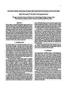
Figure 1. Symmetry of the structuring element allows only a fraction to be coded into the chromosome. The figure on the left shows the part of the structuring element coded into the chromosome, while that on the right shows how this is used to creat the entire, symmetric structuring element. This example is for a 5 × 5 structuring element, but the same general principle holds for any sized structuring element.

4.1.1. Structuring Element We restrict ourselves to flat (Function-Set Processing: FSP)19 structuring elements. We also restrict ourselves to having only 4-way symmetric (i.e. symmetric about horizontal, vertical and two diagonal axes) structuring elements, to provide a degree of rotational invariance. We predefine the overall limits of the extent of the structuring element and we allow the GA to search for any structuring element within that spatial envelope, given the symmetry constraints. The structuring element part of the chromosome is a binary string in which a one or zero represents a position that is either within or outside the structuring element’s region of support, respectively. Fig. 1 illustrates the manner in which only a small segment of a structuring element is required to be included in the chromosome, if the structuring element is to be 4-way symmetric. 4.1.2. Sequence of Spectral Morphology Operators The fundamental morphological operators are dilation and erosion. Compound operators such as closing, opening, close-opening and open-closing can be constructed from sequential application of the fundamental operators. When choosing an appropriate sequence of spectral morphology operators, there are two components to the choice: the length of the sequence and the operators employed in the sequence. We predefine a fixed sequence length and provde three operators which can be applied at each position in the sequence: spectral dilation, spectral erosion and the identity (do nothing) operator. We encode the fixed length sequence of operators with a sequence of integers which decode to dilation, erosion and the identity operator. 4.1.3. Ordering Metric The ordering metric is fixed for the sequence of spectral morphology operators. The ordering metric is applied to the collection of vectors defined by the structuring element. The ordering metric is represented in the chromosome as a single integer, which specifies one of the following ordering metrics: 1. This metric is based on comparing the absolute magnitude of the vectors in the collection (i.e. the vectors are ordered based on their Euclidean distance from the origin). 2. This metric is based on comparing the cumulative Euclidean distance between each vector and all other vectors in the collection. 3. This metric is based on comparing the Euclidean distance between each vector and the centroid of all the vectors in the collection. 4. This metric is based on the marginal ordering (i.e. each spectral band is ordered separately).

5. This metric is based on comparing the cumulative angular distance between each vector and all other vectors in the collection. 6. This metric is based on comparing the angular distance between each vector and the centroid of all the vectors in the collection. 7. This metric is based upon a cumulative “morphological” distance between each vector and all other vectors in the collection. This particular morphological distance is based on the minimum distance between bands, over all the bands. Thus, only vectors with large differences in all or most of their spectral bands will produce large values when compared with this metric. 8. This metric is based upon a “morphological” distance between each vector and the centroid of all the vectors in the collection. This particular morphological distance is also based on the minimum distance between bands. 9. This metric is based upon a slightly different “morphological” distance between each vector and the centroid of all the vectors in the collection. This morphological distance is based on the maximum distance between bands, over all the bands. Thus, vectors with large differences in at least one of their spectral bands will produce large values when compared with this metric. 10. This metric is based upon yet another “morphological” distance between each vector and the centroid of all the vectors in the collection. This morphological distance is based on the count of the number of bands for which the value at that band is greater than that of the centroid.

4.2. Genetic Algorithm The linear chromosome was constructed by concatenating all the segments for the various parameters, as described previously. For our GA implementation, we used the GAlib genetic algorithm package, written by Matthew Wall at the Massachusetts Institute of Technology.20 The criterion (fitness) which we were optimizing in the experiments we conducted was based on minimizing the total classification error. This metric is basically the same as that employed by GENIE. The fitness of a candidate solution is given by the degree of agreement between the final binary output plane and the training data. If we denote the detection rate, (fraction of “true” pixels classified correctly) as Rd and the false alarm rate, (fraction of “false” pixels classified incorrectly) as R f , then the fitness F of a candidate solution is given by F = 500(Rd + (1 − Rf )).

(1)

Thus, a fitness of 1000 indicates a perfect classification result. This fitness score gives equal weighting to type I (true pixel incorrectly labelled as false) and type II (false pixel incorrectly labelled as true) errors. Note a fitness score of 500 can be trivially achieved with a classifier that identifies all pixels as true (or all pixels as false). Thus, a fitness of 1000 indicates a perfect classification result, i.e. no training pixels in any class have been classified incorrectly, and a fitness of 0 indicates an entirely incorrect classification, i.e. no training pixels in any class have been classified correctly. The fitness calculation was made on the final output of the hybrid classifier - i.e. after the data had been processed by the spectral morphology operator, the Fisher linear discriminant and an exhaustive search for the minimum threshold value for the output of the Fisher discriminant.

5. DATA SETS AND EXPERIMENTS 5.1. Data Sets Six data sets were employed, with a broad range of spectral complexity, ranginng from simple 3-band RGB data to 480-band hyper-spectral FTIR imaging spectroscopy data.

RGB: 3-band (RGB) data were provided by the British Ministry of Defence’s Defence Science and Technology Laboratory (DSTL) (http://www.dstl.gov.uk). The original images were taken using a wet-film SLR camera from a helicopter somehwere over England. The digital data was obtained from scanning the film negatives. IKONOS: 4-band multi-spectral (red, blue, green, near infrared), 4-meter spatial resolution data from Space Imaging’s IKONOS earth imaging satellite,21 taken over the town of Los Alamos, NM, USA. Daedalus: 10-band data ranging from 0.42μm (blue) to 2.35 μm (short-wave IR) was collected over the tarmac at Nellis AFB in Nevada, using the Daedalus 1268 multi-spectral scanner (http://www.sensytech.com). These data were provided by DOE Remote Sensing Laboratory, NV, USA. Medical: 29-band histopathology image data. Images were acquired with a prototype of CRI’s 22 Nuance(tm) multispectral imaging system attached to a standard light microscope. Using liquidcrystal tunable filter technology and a 1.3-megapixel scientific-grade monochrome CCD, a spectral image data cube of 29 bands was acquired over the wavelength range 420 to 700 nm at 10-nm intervals. The specimens (generously provided by Dr. George Mutter, Brigham and Women’s Hospital, Boston) were 4-micron-thick sections of formalin-fixed, paraffin-embedded endometrium (both normal and hyperplastic) stained with standard hematoxylin and eosin dyes. AVIRIS: 224-band, Airborne Visible and InfraRed Imaging Spectrometer (AVIRIS)23 data. FTIR: 480-band data obtained using an FTIR imaging spectrometer. The imaging instrument utilizes the Michelson interferometer from a Digilab FTS6000 FTIR spectrometer to modulate the illumination source (150 W Tungsten lamp). The light source illuminates the sample and the reflected light is collected using a 50 mm camera lens and focused onto a CCD array detector (PixelFly 210xs, Cooke Corporation). The FTS6000 is operated in step scan mode at a step rate of 50 Hz. TTL signals from the commercial spectrometer are used to trigger data collection. The camera is composed of 640 x 480 pixels of 9.9 microns x 9.9 microns each. The data used in the experiments described here consisted of 480 bands, having a spectral range from 482.5 nm to 810 nm. The data had also been converted to absorbance. The image is of a sample of a CMYK map, printed on photographic paper.

5.2. Experiments Our experiments involved feature extraction tasks for a broad range of features of interest and using a set of data having a very broad range of complexity. As described above, the data sets we chose for our experiments ranged from 3-channel, standard RGB image data, through to 480-channel hyperspectral FTIR spectroscopy image data. We actually had two sets of data for each data type, one for use in the training of the algorithms, and the other for testing how well the algorithms performed on unseen (out of training sample) data. For each data set, we chose a feature in the data and had a human provide examples and counter-examples of the feature of interest. Thus, we had a two class problem for each data type: the feature of interest and the background of everything else. For each data type, this was done for the same feature in both the training and testing data sets. The following provides a description of the feature of interest in the various data sets used in these experiments.

RGB: Red cars. IKONOS: Roads. Daedalus: F16 aircraft. Medical: Endometrial glands. AVIRIS: Golf courses. FTIR: A particular type of text. As somewhat of an aside, for the medical example (finding glands in endometrial tissue), the clinical importance of these analyses is that the “gland-stroma” ratio reflects the hyperplastic process, and the higher the ratio, the more serious (and likely to progress to endometrial cancer) the lesion is. Currently, this ratio is usually estimated by eye; having a reliable automated tool could make this process less subjective and more reproducible. It should be noted the output of a spectral morphology operator has the same spectral dimension as the input data and therefore, in order to produce a classification it is necessary to feed the spectral morphology output into a suitable classifier. This is a major motivation in adopting the hybrid (spectral morphology followed by linear discriminant) approach described here. Our experiments were designed to investigate whether spatial processing in the spectral domain (i.e. spatio-spectral processing using spectral morphology) provides a benefit over processing using only the spectral information. We therefore compare the performance of our spectral morphology-based classification algorithms to that of applying the plain Fisher linear discriminant to the same data. It should also be noted that the GA’s search space includes the plain Fisher linear discriminant, due to the fact that the identity operator is one of the candidates in the spectral morphology operator gene pool. Thus, if the identity operator is chosen at every position in the sequence of spectral morpholgoy operators, the input data is passed untouched through the sequence of spectral morphology operators and into the Fisher linear discriminant, and the hybrid algorithm essentially becomes the plain Fisher linear discriminant. For our experiments we limited our search space to an operator sequence length of 1 and a maximum structuring element size of 5 × 5. Thus, our GA was permitted to search for any single spectral morphology operator (in addition to the identity) with any 4-way symmetric structuring element configuration within a 5 × 5 envelope. We used a steady-state GA having a population size of 30, for a total of 50 generations, with a crossover rate of 0.9 and a mutation rate of 0.03.

6. RESULTS Table 1 shows the parameters found by the GA for the various feature extraction problems. This information includes the spectral morphology operator, ordering metric and structuring element found for each feature extraction problem. Table 2 shows the performance of the feature extraction algorithms found during training on the various feature extraction problems for the training data sets. The performance is shown for the hybrid spectral morphology + Fisher linear discriminant algorithms and the plain Fisher linear discriminant. The performance is provided in terms of detection rate (DR), false alarm rate (FAR) and score (i.e. fitness as defined in Eq. 1, as a combination of DR and FAR). Table 3 shows the performance of the feature extraction algorithms found during training on the various feature extraction problems for the testing data sets. Again, just as for the training data sets, the performance is shown for the hybrid spectral morphology + Fisher linear discriminant algorithms and the plain Fisher linear discriminant. Figure 2 (a) shows the 56th band of the region extracted from an AVIRIS image used in training the classifiers. Figure 2 (b) shows the class labels for the image shown in Fig. 2 used during training of the classifiers. In this image white indicates pixels labelled as “true”, i.e. the golf course class, gray represents pixels labelled as “false”, i.e. the background class and black indicates pixels that have no labels assigned to them. Figure 2

Table 1: Spectral morphology operators and ordering metrics obtained by GA search for the test problems Data Type

RGB

IKONOS

Daedalus

Medical

AVIRIS

FTIR

Feature

Num. Bands

Red Cars

Roads

3

4

F16 Aircraft

Endometrial Glands

Golf Course

Printed Text

10

29

224

480

Operator

Dilation

Erosion

Erosion

Dilation

Dilation

Dilation

Metric

4

2

8

9

1

4

Structuring Element 1

0

0

0

1

0

0

0

0

0

0

0

0

0

0

0

0

0

0

0

1

0

0

0

1

1

1

1

1

1

1

0

0

0

1

1

0

0

0

1

1

0

0

0

1

1

1

1

1

1

0

1

1

1

0

1

1

1

1

1

1

1

0

1

1

1

1

1

1

1

0

1

1

1

0

1

1

1

1

1

1

1

1

1

1

1

1

0

1

1

1

1

1

1

1

1

1

1

1

1

0

1

1

1

0

1

1

0

1

1

1

0

1

0

1

1

1

0

1

1

0

1

1

1

0

1

1

1

1

1

1

1

1

1

1

1

1

1

1

1

1

1

1

1

1

1

1

1

1

1

Table 2. Performance of feature extraction algorithms on various problems, with a broad variation of spectral complexity. For training data

Data Type RGB IKONOS Daedalus Medical AVIRIS FTIR

Feature Red Cars Roads F16 Aircraft Endometrial Glands Golf Course Printed Text

Num. Bands 3 4 10 29 224 480

Fisher Linear Discriminant Score DR FAR 869.97 81.57 7.58 953.93 96.14 5.35 976.22 97.39 2.15 734.06 81.22 34.41 970.46 96.48 2.39 905.74 93.02 11.87

Spectral Score 922.13 962.00 988.48 826.79 996.42 970.88

Morphology + Fisher DR FAR 87.90 3.48 97.06 4.66 99.67 1.98 83.94 18.59 99.42 0.14 96.73 2.56

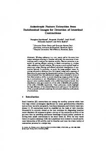
(c) shows the result of applying the hybrid spectral morphology + Fisher linear discriminant classifier to the 224-band AVIRIS image data used in training (corresponding to the region shown in Fig. 2 (a)). Figure 2 (d) shows the result of applying the plain Fisher linear discriminant classifier to the AVIRIS training data. Figure 3 (a) shows the 8th band of the region extracted from a multispectral medical image used for testing the classifiers. Figure 3 (b) shows the class labels for the image shown in Fig. 2 used for determining out-oftraining-sample peformance of the classifiers. In this image white indicates pixels labelled as “true”, i.e. the endometrial gland class, gray represents pixels labelled as “false”, i.e. the background class and black indicates

Table 3. Performance of feature extraction algorithms on various problems, with a broad variation of spectral complexity. For testing data

Data Type RGB IKONOS Daedalus Medical AVIRIS FTIR

Feature Red Cars Roads F16 Aircraft Endometrial Glands Golf Course Printed Text

Num. Bands 3 4 10 29 224 480

Fisher Linear Discriminant Score DR FAR 841.55 83.59 15.28 881.28 86.96 10.71 970.70 97.37 3.23 497.31 1.55 2.08 664.16 100.0 67.17 672.12 99.65 65.23

Spectral Score 912.72 884.00 975.07 881.03 954.74 887.16

(a)

(b)

(c)

(d)

Morphology + Fisher DR FAR 90.69 8.15 86.80 10.00 97.87 2.86 86.14 9.93 100.0 9.05 99.28 21.85

Figure 2. (a) Region of band 56 of AVIRIS data used in training. (b) Region of AVIRIS data showing class labels provided by human expert. White indicates pixels labelled as “true”, in this example being the golf course class, gray represents pixels labelled as “false”, the background class. Black indicates pixels that have no labels assigned to them. (c) Classification result from hybrid spectral morphology + Fisher linear discriminant algorithm applied to the 224-band AVIRIS image used in training. White indicates those pixels labelled as “true”, i.e. golf courses. (d) Classification result from plain Fisher linear discriminant applied to the 224-band AVIRIS image used in training. Again, white indicates those pixels labelled as “true”, i.e. golf courses.

pixels that have no labels assigned to them. Figure 3 (c) shows the result of applying the hybrid spectral morphology + Fisher linear discriminant classifier to the 29-band medical image data used for training. Figure 3 (d) shows the result of applying the plain Fisher linear discriminant classifier to the medical testing data.

7. DISCUSSION The results presented here do seem to indicate that our approach does actually provide something useful. It is interesting to note that, with regard to the ordering metrics, only 1 through 6 had been seen in the literature. However, for two of the results, other metrics were chosen during the optimization. So, this provides an indication that these “new” metrics show promise. It should also be notted that in the experiments conducted here, due to lack of available time to perform the necessary computer runs, the complexity of the spectral morphology search space was seriously reduced (only one operator and a maximum structuring element size of 5×5, together with fairly small GA runs). A significant part of the power of mathematical morphology comes about from its ability to combine fundamental operators into new operators having far greater utility than the simple operators themselves, such as opening, closing and open-closings, etc., being built up from sequences of dilations and erosions. For our experiments we did

(a)

(b)

(c)

(d)

Figure 3. (a) Band 8 of medical data used in testing. (b) Region of medical data showing class labels provided by human expert, used for determining out-of-training-sample peformance of the classification algorithms. White indicates pixels labelled as “true”, in this example being the golf course class, gray represents pixels labelled as “false”, the background class. Black indicates pixels that have no labels assigned to them. (c) Classification result from hybrid spectral morphology + Fisher linear discriminant algorithm applied to the 29-band medical image used for testing. White indicates those pixels labelled as “true”, i.e. endometrial gland. (d) Classification result from plain Fisher linear discriminant applied to the 29-band medical image used in testing. Again, white indicates those pixels labelled as “true”, i.e. endometrial gland.

not allow our search to include these more complex, compound operators, and thus our results are perhaps not quite as good as they could have been. However, given the “simplicity” of the allowable operator search space, the results are certainly interesting. Our optimization technique is set up in such a way that, by increasing the possible search space to include larger and more complex operators, the resulting larger search space still includes the search space for the simpler (and smaller) operators. Thus, if these simpler operators are indeed superior for an application, then the optimization strategy should still be able to select these operators over more complex ones. Obviously, at the same time one must also consider that as one increases the complexity of a search space, there is an increased risk of overfitting. Based on our experiments and our results we believe there are some interesting further experiments to conduct, such as the effect of increasing the optimization search space by allowing increased complexity of

the spectral morphology operators and increasing the size of the GA runs (through increasing population size, number of generations, etc.). It would also be interesting to compare the results of such experiments with other techniques that peform feature extraction using combinations of spectral and spatial information (obvious candidates being GENIE and Afreet).

8. CONCLUSIONS Our experiments have shown that, for a broad of range of problems and data types, when combined with a spectral classifier, spectral morphological operators can be useful in improving classifier performance. We have also described a method by which these spectral morphological operators can be optimized for such classification tasks.

ACKNOWLEDGMENTS We would like to thank Dr. Peter Harvey of the Defence Science and Technology Laboratory, MOD, UK, Dr. Richard Levenson of CRI Inc. of Woburn, MA, Dr. Eric Brauns of the Integrated Spectroscopy Laboratory (ISL) of Los Alamos National Laboratory, and the Department of Energy (DOE) Remote Sensing Laboratory for providing data that was used in this study. Finally we acknowledge funding from the Los Alamos ISR RD Office and from DOE’s DAPS (Deployable Adaptive Processing Systems) project.

REFERENCES 1. N. R. Harvey, J. Theiler, S. P. Brumby, S. Perkins, J. J. Szymanski, J. J. Bloch, R. B. Porter, M. Galassi, and A. C. Young, “Comparison of GENIE and conventional supervised classifiers for multispectral image feature extraction,” IEEE Trans. Geosci. and Remote Sens. 40, pp. 393–404, 2002. 2. L. J. Sartor and A. R. Weeks, “Morphological operators on color images,” J. Electronic Imaging 10(2), pp. 548–559, 2001. 3. F. Ortiz, F. Torres, J. Angulo, and S. Puente, “Comparative study of vectorial morphological operations in different color spaces,” in Proc. SPIE, 4572, pp. 259–268, 2001. 4. H. M. Al-otum, “Morphological operators for color image processing based on Mahalanobis distance measure,” Opt. Eng. 42(9), pp. 2595–2606, 2003. 5. M. Wheeler and M. A. Zmuda, “Processing color and complex data using mathematical morphology,” in Proc. IEEE National Aerospace and Electronics Conf., pp. 618–624, 2000. 6. P. Lambert and J. Chanussot, “Extending mathematical morphology to color image processing,” in Proc. Int. Conf. Color in Graphics and Image Processing, pp. 158–163, 2000. 7. J. Chanussot and P. Lambert, “Total ordering based on space filling curves for multivalued morphology,” in Mathematical Morphology and its Applications to Image and Signal Processing, H. J. A. M. Heijmans and J. B. T. M. Roerdink, eds., pp. 51–58, Kluwer Academic Publishers, 1998. 8. M. L. Comer and E. J. Delp, “Morphological operations for color image processing,” J. Electronic Imaging 8(3), pp. 279–288, 1999. 9. A. Plaza, P. Martinez, A. Gualtieri, and R. M. Perez, “Spatial/spectral identification of endmembers from AVIRIS data using mathematical morphology,” in Summaries of the XJPL Airborne Earth Science Workshop, 2001. 10. A. Plaza, P. Martinez, R. Perez, and J. Plaza, “Spatial/spectral endmember extraction by multidimensional morphological operations,” IEEE Trans. Geosci. and Remote Sens. 40(9), pp. 2025–2041, 2002. 11. A. Plaza, P. Martinez, A. Gualtieri, and R. M. Perez, “Automated identification of endmembers from hyperspectral data using mathematical morphology,” in Proc. SPIE, 4541, pp. 278–286, 2002. 12. S. Perkins, N. R. Harvey, S. P. Brumby, and K. Lacker, “Support vector machines for broad area feature classification in remotely sensed images,” in Proc. SPIE, 4381, pp. 286–295, 2001. 13. C. M. Bishop, Neural Networks for Pattern Recognition, ch. 3, pp. 105–112. Oxford University Press, 1995. 14. N. R. Harvey and S. Marshall, “Use of genetic algorithms in morphological filter design,” Signal Processing: Image Communication 8(1), pp. 55–71, 1996.

15. R. Ehrhardt, “Morphological filter design with genetic algorithms,” in Proc. SPIE, 2330, pp. 2–12, 1994. 16. W. Li, V. Haese-Coat, and J. Ronsin, “Using adaptive genetic algorithms in the design of morphological filters in textural image processing,” in Proc. SPIE, 2662, pp. 24–34, 1996. 17. P. Kraft, N. R. Harvey, and S. Marshall, “Parallel genetic algorithms in the optimization of morphological filters: a general design tool,” J. Electronic Imaging 6(4), pp. 504–516, 1997. 18. M. Hamid, N. R. Harvey, and S. Marshall, “Genetic algorithm optimization of multidimensional grayscale soft morphological filters with applications in film archive restoration,” IEEE Trans. Circuits and Systems for Video Technology 13(5), pp. 406–416, 2003. 19. P. Maragos and R. W. Schafer, “Morphological filters- part I: Their set-theoretic analysis and relations to linear shift-invariant filters,” IEEE Trans. Acoustics, Speech and Signal Processing 35, pp. 1153–1169, August 1987. 20. “GAlib home page.” http://lancet.mit.edu/ga/. 21. “Space Imaging’s IKONOS satellite web page.” http://www.spaceimaging.com/products/ikonos/index.htm. 22. “Cambridge research & instrumentation, inc. home page.” http://www.cri-inc.com. 23. “AVIRIS home page.” http://aviris.jpl.nasa.gov.