spectroscopic techniques Wavelet Transform Based on the Optimal

spectroscopic techniques

Wavelet Transform Based on the Optimal Wavelet Pairs for Tunable Diode Laser Absorption Spectroscopy Signal Processing Jingsong Li,a,* Benli Yu,a Horst Fischerb a Key Laboratory of Opto-Electronic Information Acquisition and Manipulation of Ministry of Education, Anhui University, No. 111 Jiulong Road, Hefei 230039, China b Department of Atmospheric Chemistry, Max Planck Institute for Chemistry, Mainz 55128, Germany

This paper presents a novel methodology-based discrete wavelet transform (DWT) and the choice of the optimal wavelet pairs to adaptively process tunable diode laser absorption spectroscopy (TDLAS) spectra for quantitative analysis, such as molecular spectroscopy and trace gas detection. The proposed methodology aims to construct an optimal calibration model for a TDLAS spectrum, regardless of its background structural characteristics, thus facilitating the application of TDLAS as a powerful tool for analytical chemistry. The performance of the proposed method is verified using analysis of both synthetic and observed signals, characterized with different noise levels and baseline drift. In terms of fitting precision and signal-to-noise ratio, both have been improved significantly using the proposed method. Index Headings: Laser spectroscopy; Tunable diode laser absorption spectroscopy; TDLAS; Wavelet transform; Spectroscopic applications.

INTRODUCTION Tunable diode laser absorption spectroscopy (TDLAS) is a powerful analytical technique for accurately, reliably, and continuously measuring target gas concentrations based on fundamental principles of absorption spectroscopy. Since the first demonstration of highresolution spectroscopy using a lead–tin telluride diode laser by Hinkley and coworkers at the Massachusetts Institute of Technology Lincoln laboratory in 1970,1 TDLAS has been developed for several decades. With significant performance improvements in new diode laser sources,2,3 novel laser spectroscopic techniques,4,5 and advanced signal processing methods,6 TDLAS has gradually matured for various analytical purposes. Apart from concentration, it is also possible to determine the temperature, pressure, velocity, and mass flux of the gas under observation.7,8 Just as its name implies, this Received 3 July 2014; accepted 4 September 2014. * Author to whom correspondence should be sent. E-mail: ljs0625@ 126.com. DOI: 10.1366/14-07629

496

Volume 69, Number 4, 2015

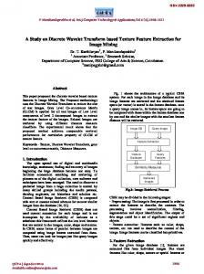
technique uses tunable diode laser sources, which offer small size, lower cost, lower power requirements, and easier tuning, as well as fast response, thus making them useful for spectroscopic applications, such as remote sensing of environmental gases and pollutants in the atmosphere, homeland security,9 industrial exhaust emissions for process control,10 and medical diagnostics such as breath analyzers,11 as well as plasma chemistry.12 Compared with classic chemical and chromatographic measurement techniques, TDLAS shows high sensitivity and selectivity, rapid responsibility, nondestructive, environmentally friendly analysis (i.e., without use of chemicals and without releasing harmful by-products into the environment), multivariate, and remote sensing. Atmospheric trace gases can be monitored with high precision, accuracy, high specificity, and fast time resolution using TDLAS from aircraft, balloons, ships, and mobile van platforms, as well as from fixed sites at remote locations.13–15 The carrier density inside the diode laser controls both the optical emission frequency and the optical emission intensity; thus if a diode laser is directly modulated using injection-current modulation to acquire the molecular absorption profile, as seen in Fig. 1 (negative correlation between detector signal and laser ramp because of negative feedback gain), then the incident laser intensity or power will also be simultaneously modulated with a similar trend. Before being processed to retrieve useful information, the raw spectrum signal must be intensity normalized and wavelength/frequency calibrated (using a Perot–Fabry etalon with a known free spectral range). Intensity normalized spectrum are obtained by dividing the raw spectrum by a baseline (i.e., the intensity that was measured during a same scan without absorbing gas in the probed area). Generally two methods have been used to obtain the baseline: (i) One spectrum synchronously acquired without target species (such as zero air) was used as a baseline with a second channel under the same optical path

0003-7028/15/6904-0496/0 Q 2015 Society for Applied Spectroscopy

APPLIED SPECTROSCOPY

FIG. 1. Typically unprocessed absorption signal, laser ramp, and Perot–Fabry interference signal in TDLAS.

length and laser beam intensity, or subsequently acquired after the sample gas in the same channel. This method is not all that reliable because global transmission may vary with time (e.g., due to pollution of windows under harsh environments) and decrease the duty cycle. Moreover, the introduction of a second channel makes the system more complicated and expensive. (ii) The baseline can be simulated from the absorption spectrum itself. A high-order polynomial function is fitted to the areas of the recorded spectrum without atmospheric absorption features. This method usually gives good results when the baseline is rather smooth and the raw spectrum has a good signal-tonoise ratio (SNR) and good resolution for absorption peaks. Since the segments containing no absorption line are often distinguished using direct visual inspection (DVI), a larger baseline-fitting error could occur for spectra with poor quality, which hampers the accurate determination of absorption line shapes, and in turn influences the final measurement precision and accuracy. In addition, this method is not suitable for processing a large number of spectra with unpredictable backgrounds, when performing time series measurements or spatial mappings in TDLAS. In recent years, wavelet transform (WT) as a powerful tool has been successfully applied to various spectroscopic techniques for signal processing,16 for example, Fourier transform infrared spectroscopy,17 laser-induced breakdown spectroscopy,18 TDLAS,19 and wavelength modulation spectroscopy,20,21 as well as Raman spectroscopy,22 mostly to show its capacity in denoising and the enhancement of SNR. However, as far as we know, there have been no previous studies on the use of wavelets in TDLAS for background removal. In this paper, we propose an adaptive method based upon discrete wavelet transform (DWT) and the choice of an optimal wavelet pair for TDLAS signal processing, involving both signal denoising and background baseline correction. In terms of fitting precision and SNR

FIG. 2. Schematic description of the Mallat algorithm for discrete wavelet transform.

improvement for molecular spectroscopy study and trace gas concentration detection, WT proved to be a powerful tool in terms of noise depression, peak shape preservation, and baseline removal.

THEORY AND METHOD In this section, only some key concepts of wavelet transform are presented. More related details of mathematical treatment may be found in the references provided along each one of the parts within this section. Subsections have been ordered according to the steps for TDLAS signal processing. Wavelet Transform Theory and Algorithm. Wavelet transform in some respects resembles the Fourier transform, in which sine and cosine are the basic analyzing functions. The multi-resolution wavelets are a family of basic functions, well localized in both time and frequency domains and based on the scaling function u(t) and the corresponding mother wavelet w(t). In practice, to realize wavelet transform with a computer, the following scaling function and the mother wavelet is often used: uj;k ðt Þ ¼ 2j=2 uð2j t k Þ

ð1Þ

wj;k ðt Þ ¼ 2j=2 wð2j t k Þ

ð2Þ

with the subscript j denoting the scale and k relating to the translation. Mallat proposed an efficient algorithm to perform the DWT,23 which provides a natural framework for understanding wavelet transform, as depicted in Fig. 2. The decomposition can be accomplished by repeating


497

a linear transformation involving two scaling functiondependent and wavelet function-dependent orthogonal filters, a low-pass filter and a high-pass filter. At each scale, the input signal is decomposed into the highfrequency component called wavelet coefficients or details coefficients (cDj) and the low-frequency component called approximation coefficients (cAj). The approximation coefficients are employed in the next scale to form a new details coefficients (cDjþ1) and approximation coefficients (cAjþ1). By increasing the decomposition level, less information will be included in the approximation coefficients. The so-called lost information between the approximation coefficients of two successive decompositions is encoded into the corresponding detail coefficients. This process can be iterated to the maximum level n, which depends on the signal length of 2n. Subsequently, the standard denoising technique operating with proper thresholding policy is applied to the wavelet coefficients for removing the noises. The denoising procedure requires the estimation of the noise level from the detail coefficients. Finally, the denoised signal can be reconstructed with the new estimated wavelet coefficients using inverse DWT. Assuming that the real TDLAS signal is f(t) and it has been corrupted by additive noise n(t), then one observes that the actual signal is y(t) = f(t) þ n(t). In DWT, the noisy signal can be described as X XX y ðt Þ ¼ aJ;k uJ;k ðt Þ þ dj;k Wj;k ðt Þ ; ðZ 2 RÞ k ¼Z

jJ k ¼Z

ð3Þ where the first and second terms represent the approximation part of the signal and the detailed part of the signal, respectively. In the wavelet multi-resolution analysis, the wavelet coefficients aJ,k and dj,k on adjacent scales are related by the decomposition. On the whole, the wavelet-based signal denoising process can be summarized in the following three steps: (1) Decompose the signal using DWT into n levels (n depending on the signal length of 2n) and obtain the empirical wavelet coefficients at each scale j (j = 1, . . ., n). (2) Threshold of the empirical wavelet coefficients using proper thresholding function, so that the estimated wavelet coefficients are obtained based on the selected threshold. (3) Reconstruct the processed signal from the thresholded wavelet coefficients at the optimal decomposition level using the inverse DWT. Denoising Using Discrete Wavelet Transform. The wavelet threshold denoising method is influenced by several key issues such as the mother wavelet, decomposition level, threshold selection, and thresholding policy.24 To determine the most appropriate wavelet for processing spectral signals, the influence of the type of wavelet on the reconstructed signal should be studied first. There are many mother wavelets available from the wavelet toolbox of commercial software, such as Matlab and Python, for example, Haar, Daubechies 1-20, Symmlet 2-20, Coif 1-5, Bior 1.1-6.8,

498


Rbio 1.1-6.8, Dmey, etc. It is worth mentioning that the purpose of an optimal filter is to recover the denoised signal without degrading the degree of approximation between the real signal and the reconstructed signal. Wavelet-based filtering is a data-dependent process. Improper choice of a mother wavelet can cause distortions and artifacts in the reconstructed signal, such as Haar wavelets (not shown here).20 The level of decomposition will also have a strong influence on the reconstructed signal. The optimal level of decomposition also should be investigated for each wavelet on the simulated signals before applying to the real signal, typically between 5 and 7. To perform the threshold denoising described above, two approaches are commonly applied to signal denoising, namely, hard thresholding or soft thresholding. The hard thresholding operation sets the wavelet coefficients smaller than the threshold to zero and keeps the values of the other wavelet coefficients. The soft thresholding operation consists of setting the wavelet coefficients smaller than the threshold to zero and shrinks the others toward zero. The hard thresholding operation keeps the amplitude constant before and after denoising, but might induce some Gibbs oscillation at the edges due to its discontinuity. The so-called soft thresholding function has the well-known and desirable properties of smoothness and adaptation, which might reduce the signal amplitude due to the constant presence of a bias at the wavelet coefficients higher than the threshold. In view of these issues, another way to achieve a trade-off between hard and soft thresholding is to use a soft-squared thresholding nonlinearity, also named a Stein estimator,25 which has been used on the signal processing in this paper. The denoising efficiency was generally evaluated in statistics by computing the SNR or the root mean square error (RMSE) between the denoised signal and the ideal one. The following equations are the definition of SNR and RMSE. fi is the noise-free signal and si is the noisy signal. 9 8 N X > > > > 2 > > fi > > = < i¼1 ð4Þ SNR ¼ 10 3 log N > > X > 2> > > > ; : ðfi si Þ > i¼1

vffiffiffiffiffiffiffiffiffiffiffiffiffiffiffiffiffiffiffiffiffiffiffiffiffiffiffiffiffiffi u N u1 X RMSE ¼ t ðfi si Þ2 N i¼1

ð5Þ

Baseline Correction Using Discrete Wavelet Transform. Before being processed to retrieve useful information, removing the baseline variations would be beneficial to the quantitation analysis of TDLAS spectra. Unlike noise, which is a high-frequency signal mainly included in the detail coefficients of the DWT, baseline variation is a low-frequency signal, belonging to the components in approximation coefficients that have similar or even larger scales compared with signal. Consequently, the baseline correction could be accomplished by removing these components in approximation coefficients using DWT. Perrin et al.26 proposed a

FIG. 3. Wavelet coefficients at different scales based on DWT.

strategy to achieve simultaneous noise and baseline removal for microchip capillary electrophoresis signal using Haar wavelets. The procedure that was applied to simultaneously remove noise and baseline was simply described as follows: At the optimal decomposition level for denoising, soft thresholding on approximation coefficients was employed for baseline correction, while hard thresholding on detail coefficients was adopted to remove noise. This strategy was exceedingly useful for dealing with baseline variations that have similar scales to signal, as shown in their work. For Raman signals with a different background, Ramos and Ruisańchez22 modified this strategy using a so-called block thresholding strategy on the detail coefficients and a same thresholding on the approximation coefficients at the optimal denoising level, and the Symmlet 8 wavelet was used in their case. But for the baseline with much larger scales than the signal, or with complicated background structures and different peak features, the optimal decomposition level for denoising was not enough for baseline

correction, and thus deeper decomposition will be needed. In spite of this, we sometimes still cannot completely separate the background contribution from the peak contribution in certain situations. Moreover, the choice of the same mother wavelet for both signal denoising and background correction might not be the optimal strategy. At least this is the case for the TDLAS signal demonstrated here. In this work, a higher decomposition level (usually the maximal decomposition level was used) than the optimal decomposition level for denoising was first performed; all detail coefficients were then set to zero. By reconstructing the signal using only the approximation coefficients, a primary background was obtained. The raw signal subtracted from the primary background will be the new input signal and is decomposed and reconstructed again. This process of the signal substitution, decomposition, and reconstruction can be repeated until an accurate background is achieved by calculating the RMSE. The repeated number of itera-


499

FIG. 4. Linear baseline correction and denoising using DWT. (a) Noisy signal with apparent baseline drift; (b) Baseline drift removed signal from (a) and noise-free signal; (c) Raw noise and wavelet-removed noise; (d) Denoised signal from (a); (e) Baseline drift removed signal from (d) and noisefree signal; (f) Raw baseline and wavelet-removed baseline.

tions needed for processing will typically depend on the background and peak features. This can be decided on a case-by-case basis according to the signal being analyzed; typically the iterative algorithm is performed within 10 iterations. Figure 3 presents a typical application of signal decomposition at different scales based on DWT. From this figure, we can see that the low-frequency signal cA10 nearly holds back the pattern of baseline with larger scale. Meanwhile cD1, cD2, and cD3 contain the main white noises of different high frequencies. The details on cD4 include both the noise contribution and the peak contribution. Furthermore, the medium-frequency signal peaks are correspondingly distributed in the details coefficients under higher levels of cD5–cD10, which strongly depend on the choice of mother wavelet.

RESULTS AND DISCUSSION Simulated Data. To test the proposed algorithm, simulated data with the known background and absorption peaks are first applied. The simulated spectra (typically 1024 sampling points) are the sum of linear or curved background, analytical absorption signal, and random noise. The signals were chosen as the representatives mainly for two reasons: (i) The noise was

500


prominent compared with the peaks. It would be reliable to show the denoising effect using DWT. (ii) Peak and baseline conditions were varied in these signals, for example, linear or curved background occurred often in the TDLAS signal; overlapped or independent peaks with similar or divergent height would be convenient to monitor the preservation of peak shape. After many experimental trials with each wavelet family, we found that it is hard to say which wavelet is preferable for denoising, since sometimes the difference of the best SNR obtained between the so-called optimal wavelet and others is really small, as demonstrated in our previous work.18 In general, the wavelet Daubechies 7 (db7) was found to be a good candidate for denoising TDLAS signals, and the optimal decomposition levels are slightly shifted between level 5 and 7 following the variation of the SNR. Unlike denoising, better performances for background correction that were obtained with wavelet bior2.2 and bior3.3 can probably be attributed to their features, which can better reproduce the baseline, which constituted the major part of the signals. Typically, 10 iterations for baseline removal can provide a satisfactory result. Therefore, the best wavelet pairs of db7 and bior2.2 (or bior3.3) are widely adopted for TDLAS signal processing in this work.

FIG. 5. Nonlinear baseline correction and denoising using DWT. (a) Noisy signal with apparent baseline drift; (b) Baseline drift removed signal from (a) and noise-free signal; (c) Raw noise and wavelet-removed noise; (d) Denoised signal from (a); (e) Baseline drift removed signal from (d) and noise-free signal; (f) Raw baseline and wavelet-removed baselines with different iterations.

Figure 4a presents a simulated TDLAS absorption spectroscopy, which was synthesized by adding a linear baseline drift and a proper noise to the absorption signal. This kind of baseline drift occurred often in the TDLAS system due to the inherent modulating characteristic of diode lasers. Even though the background drift has been effectively corrected with one time iteration using the proposed method at the maximal decomposition level of 10 with wavelet bior2.2, five iterations provide highly accurate background information. The correlations between the corrected and original noisefree signal are quite good after the elimination of the uneven baseline background as shown in Fig. 4b. It clearly shows that no primary useful information is lost in the whole processing procedure except the noise (see Fig. 4c) and the background information. Indeed, the whole processing procedure could also be effectively conducted in an alternative way. The noisy signal in Fig. 4a was first denoised using wavelet db7 at optimal decomposition level of 6 as demonstrated in Fig. 4d. The baseline drift was then removed by zeroing all approximation coefficients at the maximum decomposition level of 10 with five iterations (see Fig. 4e and Fig. 4f). Finally, the SNR was enhanced by a factor of over 8.

Figure 5a shows another simulated TDLAS absorption spectroscopy, which was synthesized by adding a big nonlinear baseline drift and a notably high noise to the absorption signal. This kind of baseline drift and poor SNR occurred often in practical applications under harsh environmental conditions, close to the detection limit level or the system. Under these conditions, it is difficult to distinguish the segments containing no absorption line with direct visual inspection; a larger baseline-fitting error will be induced using simple manual operation. As demonstrated here, using the proposed processing algorithm with the wavelet pairs of db7 and bior3.3, the background was effectively corrected while preserving primary useful information, and the SNR was also significantly improved, which is highly useful for subsequent spectral analysis. Analogously, the processing procedure can be realized in reverse order (a ! d ! e). As can be seen here, one time iteration is absolutely deficient for accurate background correction. Considering the poor spectral signal, the final results obtained using the proposed algorithm with 10 iterations are acceptable. Experimental Data. Based on the processing results of the synthetic signals, the proposed algorithm with the optimal wavelet pairs of db7 and bior2.2 (or bior3.3),


501

FIG. 6. Experimentally raw absorption spectra of water between 3788.65 and 3789.05 cm1 at different pressures (upper panel), the lower panel shows the corresponding Transmittance processed with the proposed algorithm.

decomposition level of 6 and 10, was finally applied to the real TDLAS spectral signals for signal denoising and background correction, respectively, for molecular spectroscopy study and trace gas concentration measurement. To perform precise line shape studies, it is necessary to have enough spectral SNR; thus spectroscopic parameters can be retrieved with high precision and accuracy. For this purpose, a series of experimental spectra of line transitions of H2O between 3788.65 cm1 and 3789.05 cm1 under different pressures between 0 and 10 mbar are recorded with water in natural abundance, as shown in Fig. 6. With the proposed algorithm with the wavelet pairs of db7 and bior2.2 for the signal denoising and baseline removal, respectively, the standard Gaussian model (y(x) = y0 þ A/[w(p/2)1/2] exp[2((x xc)/w)2]) is then used to fit the experimental H2O absorption spectra for line intensity determination. To determine absolute line intensity, the H2O absorbance was numerically integrated over the entire spectral contour, the fitted integrated absorbance area A was divided by the product of the H2O concentration and the path length to obtain the line intensity at experimental temperature, then converted to the standard temperature

502


using the lower state energy and the vibrational and rotational partition functions for intercomparison. A detailed description of the multi-peaks fitting procedure used for the analysis of the spectra and the data reduction can be found in related publications.27 For clarity, Fig. 7 shows the application of the proposed algorithm for baseline correction and noise removal on a H2O absorption spectrum with a pressure of 0.93 mbar. For comparison, the processed signal using the DVI method mentioned above and the corresponding Gaussian fit are also provided (middle panel). The fitted parameters are inset in the corresponding panel. It is worth noting that a H2O weak absorption line located at 3788.75613 cm1 with a line intensity of 3.151 3 1025 reported in the latest HITRAN12 database28 can be clearly observed after the application of the wavelet–denoising technique, as shown in Fig. 7 (lower panel). Finally, three absolute line intensities achieved with both methods are summarized in Table 1 and compared with the HITRAN12 database. For each line, the error corresponds to one standard deviation obtained by averaging the different measurements. The discrepancy between both methods and the HITRAN12

FIG. 7. Upper panel, experimental spectrum of H2O (pressure = 0.93 mbar; path length = 12 m; temperature = 293.45 K) and the baseline determined using DWT; Middle panel, baseline drift removed absorption signal using the DVI method and the corresponding Gaussian fit; Lower panel, baseline drift rand noise removed absorption signal using DWT with the wavelet pairs of db7 and bior2.2 and the corresponding Gaussian fit, for clarity, zoom-in data near 3788.76 cm1 illustrate a very weak absorption line.

data are within 61.5%. The overall agreement is satisfactory within experimental measurement uncertainty and considering the weakness of the line intensities measured with water in natural abundance. However, the uncertainty has been significantly improved using the proposed method based on DWT, which indicates the potential errors from artificial factors can be effectively avoided, as the non-absorption baseline segments are completely defined by hand and with experience in the DVI method. For further evaluation of the proposed DWT algorithm and the commonly used DVI method for trace gas

concentration measurements, a series of CO2 spectra near 4845.64 cm1 with a certain mixing ratio (approximately 1%) in air were recorded under different pressures, as shown in Fig. 8. Before fitting the spectra to predict the concentration of the absorbing species, both DVI and DWT are used to process the original signals. The measured TDLAS signals are exceedingly noisy, especially corrupted the optical etalon fringes, and with a big baseline drift (see Fig. 9). Note that the wavelet pairs of db7 and bior3.3 were used here due to the nonlinear background baseline. For clarity, a zoomin data of baseline before and after the use of the

TABLE I. Absolute line intensities for H2O isotopes at 296 K determined with two different processing methods and comparison with HITRAN12 database. S (1023 cm1/(cm2 molecule) Isotope H217O H216O H218O

Position (cm1)

DVI

% Unc.

% Disc.

DWT

% Unc.

% Disc.

HITRAN12

3788.78518 3788.80964 3788.91246

2.089 0.922 4.235

0.38 0.96 0.43

1.36 1.49 0.59

2.091 0.945 4.265

0.15 0.42 0.19

1.46 0.97 0.12

2.061 0.9359 4.260

Notes: the wavenumbers of the line positions (in cm1) are taken from the HITRAN12 database. The reported uncertainty in %Unc. corresponds to one standard deviation obtained by averaging the different measurements. %Disc. is the percentage ratio [(this work HITRAN12)/HITRAN12] 3 100.


503

FIG. 8. Experimentally raw absorption spectra of carbon monoxide near 4845.64 cm1 at different pressures (upper panel); the lower panel shows the corresponding transmittance processed with the proposed algorithm.

proposed algorithm (upper panels) illustrates the detailed comparison. As can be seen, after the application of wavelet filtering, the annoying etalon fringes that often occurred in the TDLAS system have been significantly removed. The calculated SNR in DVI and DWT are 131.3 and 781.8, respectively. Thus, an SNR enhancement factor of approximately 6 is obtained. These results prove that the proposed algorithm in this work is a highly effective signal-processing tool not only for common Gaussian noise but also for optical etalon fringes. Moreover, the background drift was effectively correct while preserving primary useful information, which is good for quantitative analysis. Taking some spectroscopic parameters from the HITRAN12 database and experimental conditions, a Voigt model was used to retrieve CO2 mixing ratios. Finally, the fitted CO2 concentrations in both cases are close to the real values due to the high-concentration samples used. However, the proposed algorithm based on DWT provides a better performance in terms of the fitting errors and processing speed, as shown in Fig. 10.

504


From this figure, the fit precision enhancement factor between 1.5 and 3.5 depending on noisy spectral characteristics was obtained. Indeed, we found that the proposed algorithm shows better performance in both measurement precision and accuracy for spectral signals with poor quality, except the advantage of high processing efficiency.

CONCLUSION In summary, the proposed algorithm for choosing the best wavelet pairs based on DWT was used as a powerful tool for TDLAS signal processing. The performance of the proposed method is verified using analysis of both synthetic and observed signals, characterized with different noise levels and baseline drift. In terms of fitting precision and spectral SNR, both have been improved significantly using the proposed method, which is extremely useful for quantitative analysis. Compared with the commonly used DVI method, the proposed algorithm shows better relative performance

FIG. 9. (a) Experimental spectrum of CO2 (pressure = 140 mbar; path length = 4800 cm; mixing ratio = 1.0%; Temperature = 292.95 K) and wavelet– denoised signal; (b) Baseline drift removed transmittance signals using DVI and DWT, as well as the Voigt fit; (c) DWT removed noise; (d) DWT removed baseline with noise and DVI removed baseline. Parts of the ‘‘baselines’’ are expanded for clarity and statistical noises are also provided in the inset.

and stability. The advantages revealed in this paper exhibited a promising future for DWT’s application to batch processing of TDLAS spectra for molecular spectroscopy study and trace gases detection.

FIG. 10. The fitting error for CO2 concentration measurements in both cases (square, the common DVI method; circle, the proposed algorithm based on DWT) as a function of total sample pressures.

ACKNOWLEDGMENTS This work was supported in part by Anhui University Personnel Recruiting Project of Academic and Technical Leaders under Grant 10117700014, the Natural Science Fund of Anhui Province under Grant 1508085MF118, the National Natural Science Foundation of China under Grant 61440010, and the key Science and Technology Development Program of Anhui Province (project execution starting 2015). 1. E.D. Hinkley. ‘‘High-Resolution Infrared Spectroscopy with a Tunable Diode Laser’’. Appl. Phys. Lett. 1970. 16: 351-354. 2. P. Werle. ‘‘A Review of Recent Advances in Semiconductor Laser Based Gas Monitors’’. Spectrochim. Acta, Part A. 1998. 54(2): 197236. 3. P. Werle, F. Slemr, K. Maurer, R. Kormann, R. Mucke, B. Janker. ‘‘Near- and Mid-infrared Laser-Optical Sensors for Gas Analysis’’. Opt. Las. Eng. 2002. 37(2-3): 101-114. 4. G. Berden, R. Peeters, G. Meijer. ‘‘Cavity Ring-Down Spectroscopy: Experimental Schemes and Applications’’. Int. Rev. Phys. Chem. 2000. 19(4): 565-607. 5. J.S. Li, W. Chen, B. Yu. ‘‘Recent Progress on Infrared Photoacoustic Spectroscopy Techniques’’. Appl. Spectrosc. Rev. 2011. 46(6): 440471. 6. P. Werle, P. Mazzinghi, F. D’Amato, M. De Rosa, K. Maurer, F. Slemr. ‘‘Signal Processing and Calibration Procedures for in Situ Diode-Laser Absorption Spectroscopy’’. Spectrochim. Acta, Part A. 2004. 60(8-9): 1685-1705. 7. L.C. Philippe, R.K. Hanson. ‘‘Laser Diode Wavelength-Modulation Spectroscopy for Simultaneous Measurement of Temperature, Pressure, and Velocity in Shock-Heated Oxygen Flows’’. Appl. Opt. 1993. 32(30): 6090-6103.


505

8. M.S. Zahniser, D.D. Nelson, J.B. McManus, P.L. Kebabian, D. Lloyd. ‘‘Measurement of Trace Gas Fluxes Using Tunable Diode Laser Spectroscopy’’. Philos. Trans. R. Soc., A. 1995. 351(1696): 371-382. 9. M.W. Sigrist. ‘‘High Resolution Infrared Laser Spectroscopy and Gas Sensing Applications’’. In: M. Quack, F. Merkt, editors. Handbook of High-Resolution Spectroscopy. Chichester, UK: John Wiley and Sons Ltd., 2011. 10. M. Lackner. ‘‘Tunable Diode Laser Absorption Spectroscopy (TDLAS) in the Process Industries—A Review’’. Rev. Chem. Eng. 2007. 23(2): 65-147. 11. T.H. Risby, S.F. Solga. ‘‘Current Status of Clinical Breath Analysis’’. Appl. Phys. B. 2006. 85(2-3): 421-426. 12. J. Ro¨pcke, G. Lombardi, A. Rousseau, P.B. Davies. ‘‘Application of Mid-Infrared Tuneable Diode Laser Absorption Spectroscopy to Plasma Diagnostics: A Review’’. Plasma Sources Sci. Technol. 2006. 15(4): S148-S168. 13. A. Fried, B. Henry, B. Wert, S. Sewell, J.R. Drummond. ‘‘Laboratory, Ground-Based and Airborne Tunable Diode Laser Systems Performance Characteristics and Applications in Atmospheric Studies’’. Appl. Phys. B. 1998. 67(3): 317-330. 14. J.S. Li, W. Chen, H. Fischer. ‘‘Quantum Cascade Laser Spectrometry Techniques: A New Trend in Atmospheric Chemistry’’. Appl. Spectrosc. Rev. 2013. 48(7): 523-559. 15. L. Zhang, G. Tian, J.S. Li, B. Yu. ‘‘Current Laser Spectroscopy Techniques—Selected Applications Involving Quantum Cascade Laser’’. Appl. Spectrosc. 2014. 68(10): 1095-1107. 16. J.S. Li, B. Yu, W. Zhao, W. Chen. ‘‘A Review of Signal Enhancement and Noise Reduction Techniques for Tunable Diode Laser Absorption Spectroscopy’’. Appl. Spectrosc. Rev. 2014. 49(8): 666691. 17. B.K. Alsberg, A.M. Woodward, M.K. Winson, J. Rowland, D.B. Kell. ‘‘Wavelet Denoising of Infrared Spectra’’. Analyst. 1997. 122: 645652. 18. B. Zhang, L. Sun, H. Yu, Y. Xin, Z. Cong. ‘‘Wavelet Denoising Method for Laser-Induced Breakdown Spectroscopy’’. J. Anal. At. Spectrom. 2013. 28: 1884-1893. 19. I. Mappe-Fogaing, L. Joly, G. Durry, N. Dumelie´, T. Decarpenterie, J. Cousin, B. Parvitte, V. Zeńinari. ‘‘Wavelet Denoising for Infrared Laser Spectroscopy and Gas Detection’’. Appl. Spectrosc. 2012. 66(6): 700-710.

506


20. J.S. Li, U. Parchatka, H. Fischer. ‘‘Applications of Wavelet Transform to Quantum Cascade Laser Spectrometer for Atmospheric Trace Gas Measurements’’. Appl. Phys. B. 2012. 108(4): 951-963. 21. C.T. Zheng, W. Ye, J. Huang, T. Cao, M. Lv, J.M. Dang, Y.D. Wang. ‘‘Performance Improvement of a Near-Infrared CH4 Detection Device Using Wavelet-Denoising-Assisted Wavelength Modulation Technique’’. Sens. Actuators, B. 2014. 190: 249-258. 22. P.M. Ramos, I. Ruisańchez. ‘‘Noise and Background Removal in Raman Spectra of Ancient Pigments Using Wavelet Transform’’. J. Raman Spectrosc. 2005. 36(9): 848-856. 23. S.G. Mallat. ‘‘A Theory for Multiresolution Signal Decomposition: The Wavelet Representation’’. IEEE Pattern Analysis and Machine Intelligence. 1989. 11(7): 674-393. 24. L. Pasti, B. Walczak, D.L. Massart, P. Reschiglian. ‘‘Optimization of Signal Denoising in Discrete Wavelet Transform’’. Chemom. Intell. Lab. Syst. 1999. 48(1): 21-34. 25. D.L. Donoho, I.M. Johnstone. ‘‘Adapting to Unknown Smoothness via Wavelet Shrinkage’’. J. Am. Stat. Assoc. 1995. 90: 1200-1224. 26. C. Perrin, B. Walczak, D.L. Massart. ‘‘The Use of Wavelets for Signal Denoising in Capillary Electrophoresis’’. Anal. Chem. 2001. 73(20): 4903-4917. 27. J.S. Li, L. Joly, J. Cousin, B. Parvitte, B. Bonno, V. Zeninari, G. Durry. ‘‘Diode Laser Spectroscopy of Two Acetylene Isotopologues (12C2H2, 13C12CH2) in the 1.533 lm Region for the Phobos-Grunt Space Mission’’. Spectrochim. Acta, Part A. 2009. 74(5): 1204-1208. 28. L.S. Rothman, I.E. Gordon, Y. Babikov, A. Barbe, D. Chris Benner, P.F. Bernath, M. Birk, L. Bizzocchi, V. Boudon, L.R. Brown, A. Campargue, K. Chance, E.A. Cohen, L.H. Coudert, V.M. Devi, B.J. Drouin, A. Fayt, J.-M. Flaud, R.R. Gamache, J.J. Harrison, J.-M. Hartmann, C. Hill, J.T. Hodges, D. Jacquemart, A. Jolly, J. Lamouroux, R.J. Le Roy, G. Li, D.A. Long, O.M. Lyulin, C.J. Mackie, S.T. Massie, S. Mikhailenko, H.S.P. Mu¨ller, O.V. Naumenko, A.V. Nikitin, J. Orphal, V. Perevalov, A. Perrin, E.R. Polovtseva, C. Richard, M.A.H. Smith, E. Starikova, K. Sung, S. Tashkun, J. Tennyson, G.C. Toon, V.G. Tyuterev, G. Wagner. ‘‘The HITRAN 2012 Molecular Spectroscopic Database’’. J. Quant Spectrosc. Radiat. Transfer. 2013. 130: 4-50.