SPICE: Simulated Pore Interactive Computing Environment Shantenu Jha
Peter Coveney
Matt Harvey
Centre for Computational Science, University College London, 20 Gordon Street, London, WC1H0AJ, United Kingdom
Centre for Computational Science, University College London, 20 Gordon Street, London, WC1H0AJ, United Kingdom
Centre for Computational Science, University College London, 20 Gordon Street, London, WC1H0AJ, United Kingdom
[email protected]
[email protected]
[email protected]
ABSTRACT SPICE aims to understand the vital process of translocation of biomolecules across protein pores by computing the free energy profile of the translocating biomolecule along the vertical axis of the pore. Without significant advances at the algorithmic, computing and analysis levels, understanding problems of this size and complexity will remain beyond the scope of computational science for the foreseeable future. A novel algorithmic advance is provided by a combination of Steered Molecular Dynamics and Jarzynski’s Equation (SMD-JE); Grid computing provides the required new computing paradigm as well as facilitating the adoption of new analytical approaches. SPICE uses sophisticated grid infrastructure to couple distributed high performance simulations, visualization and instruments used in the analysis to the same framework. We describe how we utilize the resources of a federated trans-Atlantic Grid to use SMD-JE to enhance our understanding of the translocation phenomenon in ways that have not been possible until now.
1.
INTRODUCTION
The transport of biomolecules like DNA, RNA and polypeptides across protein membrane channels is of primary significance in a variety of areas. For example, gene expression in eukaryotic cells relies on the passage of mRNA through protein complexes connecting the cytoplasm with the cell nucleus. Although there has been a flurry of recent activity, both theoretical and experimental [1, 2] aimed at understanding this crucial process, many aspects remain unclear. SPICE aims to understand the vital process of translocation of biomolecules across protein pores in ways that have not been possible until now by using sophisticated grid infrastructure to effectively utilise the computational resources of a federated trans-Atlantic Grid and to facilitate novel analysis techniques. The details of the interaction of a pore with a translocating biomolecule within the confined geometries are critical in
Permission to make digital or hard copies of all or part of this work for personal or classroom use is granted without fee provided that copies are not made or distributed for profit or commercial advantage and that copies bear this notice and the full citation on the first page. To copy otherwise, to republish, to post on servers or to redistribute to lists, requires prior specific permission and/or a fee. SC| 05 November 12-18, 2005, Seattle, Washington, USA Copyright 2005 ACM 1-59593-061-2/05/0011 ...$5.00.
determining macromolecular transport across a membrane. The interaction details can be captured best by fully atomistic simulations. The first fully atomistic simulations of the hemolysin pore have appeared very recently [3]. They address however, only static properties - structural and electrostatic - and have not attempted to address the dynamic properties of the translocating DNA. The lack of more attempts at atomistic simulations of the translocation process is due in part to the fact that the computational requirements for simulations of systems of this size for the required timescales have hitherto not been possible. For example, the time scale for DNA translocation is of the order of tens of microseconds. Simulating such long timescales for large system sizes (275,000 atoms and upwards) is not possible with standard molecular dynamics approaches. Relying only on Moore’s law (simple speed doubling every 18 months) we are still a couple of decades away from a time when such simulations may become routine.
2.
NOVEL ALGORITHMS AND COMPUTING PARADIGM
To enhance our understanding there is a need now to adopt new algorithmic approaches in conjunction with new computing paradigms, as without significant advances at the algorithmic, computing and analysis levels, understanding problems of this nature will remain beyond the scope of computational biologists. In this context, a novel algorithmic advance is provided by a combination of Steered Molecular Dynamics (SMD) and Jarzynski’s Equation [4]; Grid computing provides the required new computing paradigm as well as facilitating the adoption of new analytical approaches. The application of an external force in a SMD simulation increases the timescale that can be simulated up to and beyond microseconds, whilst Jarzynski’s Equation provides a means of computing the equilibrium free-energy profile (FEP) in the presence of non-equilibrium forces. Thus, SMD simulations provide a natural setting to use Jarzynski’s equality, and hence the combined approach is referred to as the SMD-JE approach [5]. The PMF (Φ) is defined as the free energy profile (FEP) along a well defined reaction coordinate. By computing the PMF for the translocating biomolecule along the vertical axis of the protein pore, significant insight into the translocation process can be obtained. Rather than a single detailed, long running simulation over physical timescales of a few microseconds (the typical time to solution for which will
(a)
(b)
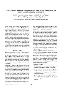
Figure 1: Snapshot of a single stranded DNA beginning its translocation through the alpha-hemolysin protein pore which is embedded in a lipid membrane bilyaer. Water molecules are not shown. Fig. 1b is a cartoon representation showing the seven fold symmetry of the hemolysin protein and the beta-barrel pore. be months to years on one large supercomputer), SMD-JE permits a decomposition of the problem into a large number of simulations over a coarse grained physical timescale with limited loss of detail. Multiple SMD-JE non-equilibrium simulations of several million time-steps (the equivalent of several nanosecond equilibrium simulations) can be used to study processes at the microsecond timescale. In order to realistically benefit from this approach, however, it is critical to find the values of the parameters that provide an “optimal PMF”. These parameters are the pulling velocity (v) and spring constant (κ) of the pulling atom to the SMD atoms. A rigorous analytic relationship between the combined statistical and systematic fluctuations of the PMF and the values of v and κ does not exist, thus, there is a need to determine the parameter values which will minimize systematic and statistical errors. It is the scientific aim of our Challenge entry to determine the values of the spring constant (κ) and pulling velocity (v) which when used to compute the PMF of DNA translocating along the axis of the pore provide an optimal PMF, viz., a balance between systematic and statistical errors for a given computational cost.
Grid computing: A suitable computing paradigm When formulated as an SMD-JE problem there is an intrinsic ability to decompose an otherwise very substantial problem into smaller problems of shorter duration. We use the capabilities developed by the RealityGrid project [6, 7, 8] to make the SMD-JE approach amenable to an efficient solution on the Grid, by using the ability provided by the Grid to easily launch, monitor and steer a large number of
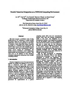
parallel simulations. The RealityGrid steering framework the architecture of which is outlined in Fig. 2a - has also enabled us to easily introduce new analysis and intuition building approaches; in particular, here we make use of haptic devices within the framework for the first time as if they were just additional computing resources. We use the infrastructure consisting of a distributed set of supercomputers - on both the UK National Grid Service as well as the US TeraGrid - for simulations, plus a dedicated visualization resource (SGI Prism) at UCL. The visualization engine is connected to the HPC resources in the UK and to the TeraGrid resources via Starlight in Chicago using a dedicated optically switched network called UK Light [9], which ensures a dedicated low latency, high speed network connection between the simulation and visualization. The haptic is connected to the SGI Prism through multi-Gigabit LAN. The resources used and shown in Fig. 2b are grid enabled in the sense of using Globus toolkit version 2 (GT2). The ability to distribute over a federated grid enables greater resource utilization as well as a single uniform interface. Hiding the heterogeneity of different resources is a major convenience for the scientist who doesn’t now have to worry about site-specific issues.
3.
SIMULATION METHOD AND ANALYSIS
The first stage is to use “static” visualization (visualizations not coupled to running simulations) to understand the structural features of the pore. However, the need to understand the functional consequences of structure, as well
(a)
(b)
Figure 2: Schematic architecture of an archetypal RealityGrid steering configuration is represented in Fig. 2a . The components communicate by exchanging messages through intermediate grid services. The dotted arrows indicate the visualizer sending messages directly to the simulation, which is used extensively here. Fig. 2b shows the network diagram highlighting the distributed infrastructure used. The double headed arrows indicate the point-to-point connections on the optically switched network - UKLight. The haptic is co-located with the visualization resource (SGI Prism). as the desire for information on forces and dynamic responses, requires the coupling of simulations to the visualizations. These are referred to as interactive molecular dynamics (IMD). Given the size of the model, in order that the simulation can compute forces quick enough so as to provide the scientist with any sense of interactivity typically requires performing simulations on 256 processors. These initial simulations along with real-time interactive tools are used to develop a qualitative understanding of the forces and the DNA’s response to forces. This qualitative understanding helps in choosing the initial range of parameters over which we will try to find the optimal value. IMD simulations are then extended to include haptic devices to get an estimate of force values as well as to determine suitable constraints to place. Checkpoint and cloning of simulations features provided by the RealityGrid infrastructure can also be used for verification and validation tests without perturbing the original simulation and for exploring a particular confirguration in greater detail. In interactive mode, the user sends data back to the simulation running on a remote supercomputer, via the visualizer, so that the simulation can compute the changes introduced by the user. When using 256 processors (or more) of an expensive high-end supercomputer it is not acceptable that the simulation be stalled (or even slowed down) due to unreliable communication between the simulation and the visualization - a general purpose network is not acceptable. Thus advanced (optically switched) networks that ensure schedulable capacity for high rate/high volume communications, and well bounded quality of service in terms of packet latency, jitter and packet loss are critical in such interactive scenarios. Once we have gathered sufficient insight from the interactive phase, we proceed to the batch phase. We used the grid infrastructure in Fig. 2b, to perform to completion 72
parallel MD simulations in under a week with each individual simulation running on 128 or 256 processors (depending upon the machine used). This required approximately 75,000 CPU hours: it is unlikely that such computations would be possible in under a week without a grid infrastructure in place. Our approach thus advances high performance computing into a new domain by using the same grid middleware to integrate high-performance computing, visualization and instrumentation within the same framework. This facilitates the solution of a problem that would otherwise probably not be possible. We now present some results to substantiate this claim.
4.
RESULTS
Before we present the results, it is important to understand the individual dependence of the PMF on the variable parameters. This emphasises the subtle interplay between statistical and systematic errors and the fact that there is no analytical method that provides a direct means to determine the best parameters to use to compute the PMF.
4.1
Choice of the sub-trajectory length
We are interested in the PMF along the entire axis of the approximately cylindrical pore. In general, the further the center of mass (COM) of the SMD atoms from its initial position, the greater the statistical and systematic errors; hence when the PMF is required over a long trajectory, it is advantageous to break up a single long trajectory into smaller trajectories. Once again there is no information upfront on the optimal length of a sub-trajectory. As the parameter values used in the computation of the final PMF need to be the same for all sub-trajectories, we choose a sub-trajectory of length 10˚ A close to the centre of the pore. In addition to helping lower the computational requirement,
Single Samples at κ= 10pN/Å
80 60 40 20 0 −20 −40 −60 −80 −100
30 20 Φ (Kcal/mol)
Φ (Kcal/mol)
Single Samples at v=12.5 Å/ns
κ=1000 κ=100 κ=10 0
1
2
10 0 −10
v=12.5 v=25 v=50 v=100
−20 −30 3
4
5
6
7
8
9
10
2
displacement of COM (Å)
3
4
5 6 7 8 displacement of COM (Å)
(a)
9
10
(b)
Figure 3: Fig. 3(a) shows the fluctuations of the PMF for individual trajectories with the same pulling velocity but different values of κ. The fluctuation in the PMF between trajectories with different κ values is significantly larger than the fluctuations in the PMF between different trajectories of the same values of κ. Fig. 3(b) shows how the PMF fluctuates when the pulling velocity is varied. It is not obvious how (and when) the PMF values change with pulling velocity. this has the advantage of being most likely to be free of boundary effects and is probably the most representative sub-trajectory.
4.2
Choice of the force constant
The proper choice of the force constant (κ) of the spring is important. Intuitively the force constant is a measure of how strongly the SMD atoms are coupled to the “fictitious” pulling atom. It needs to be large enough that the SMD atoms respect the constraints of the pulling atom, but at the same time it must not be too large or else the the PMF will become too noisy. This can be seen very clearly in Fig. 3(a), where the fluctuations for κ = 1000pN/˚ A. are extremely large, but far less for κ = 10 pN/˚ A. However, for κ =10pN/˚ A the SMD atoms are almost un-coupled to the pulling atoms which results in a large variation in the space sampled and resulting PMFs for the different v values. as can be seen in Fig. 4(a).
4.3
Choice of the pulling velocity
Given that the initial and final coordinates are well defined, the larger v, the smaller the computational time required for a single simulation. Thus the number of samples that can be simulated for a fixed computational cost is greater for larger v. It would seem to be beneficial to always opt for a larger number of samples, so as to reduce the statistical fluctuations. This proves to be incorrect, however, for too large a velocity produces “irreversible work” which results in deviations from the equilibrium PMF (the putatively correct PMF). As Fig. 3b shows, too large a velocity can be a major source of systematic error, as the quicker the DNA is pulled through the pore in the simulations, the less time it has to “sample correctly” the possible configurations. In the extreme limit of adiabatic translocation the PMF generated will be accurate. In general the slower the
v, the more accurate the sampling; however this can’t be quantified easily, and a doubling of v could result either in an unchanged PMF or possibly a highly inaccurate PMF. It is important to normalize the statistical error for the difference in computational requirements. Thus in the computational time that one sample at a v of 12.5˚ A/ns can be generated, eight samples at a v of 100˚ A/ns can be generated. Thus, the statistical √ error of a set of samples of the former should be set to be 8 of the latter. The statistical error bars in Fig. 4 have been normalized to account for different computational costs. The signal to noise ratio for κ =1000pN/˚ A is the lowest of all κ values, as seen in Fig. 4c. The statistical fluctuations are sufficiently large to swamp out any distinction between the PMFs at different velocities, thus rendering κ =1000pN/˚ A unsuitable. Although the PMFs computed using κ =10pN/˚ A have the least statistical noise, this simulation is most susceptible to systematic errors, i.e., the deviation from the close to equilibrium PMF (here that of v=12.5˚ A/ns) is larger and takes place sooner. To appreciate this, notice the PMFs for 12.5 and 25˚ A/ns for both κ = 10 and 100pN/˚ A. For κ =100pN/˚ A, they continue to overlap while for κ =10 they acquire different values once the COM has been displaced more than 6˚ A from the starting point. Also, given that the increase in statistical noise is marginal in choosing κ =100 over κ =10, κ =100 is the better choice. For κ = 100 there is no perceptible difference between the normalized statistical errors between v =12.5 and v =25˚ A/ns, hence based upon our analysis, it is best to use κ =100pN/˚ A and v=12.5˚ A/ns to compute the PMF.
5.
DISCUSSION
We discuss two potential drawbacks of our approach: Firstly, it does not provide any assurance that we have found the “globally optimal” parameters. The optimal values that
Φ (Kcal/mol)
κ = 10 pN/Å 60 40 20 0 −20 −40 −60 −80 −100 −120 −140
v = 12.5 v= 25 v = 50 v = 100 1
2
3
4 5 6 7 8 displacement of COM (Å)
9
10
9
10
9
10
9
10
(a)
Φ (Kcal/mol)
κ = 100 pN/Å 60 40 20 0 −20 −40 −60 −80 −100 −120 −140 −160
v = 12.5 v = 25 v = 50 v = 100 0
1
2
3 4 5 6 7 8 displacement of COM (Å)
(b)
κ = 1000pN/Å 50
Φ (Kcal/mol)
0 −50 −100 v = 12.5 v= 25 v = 50 v = 100
−150 −200 0
1
2
3 4 5 6 7 8 displacement of COM (Å)
(c)
v = 12.5 Å/ns 40 20 Φ (Kcal/mol)
0 −20 −40 −60 −80
κ = 10 κ = 100 κ = 1000
−100 −120 0
1
2
3 4 5 6 7 8 displacement of COM (Å)
(d) Figure 4: Plots showing the calculation of the optimal parameters (κ, v) based upon set statistical and systematic errors.
we’ve determined are a function of the set over which we’ve searched - which in turn is partially determined by insight gained during the real-time visualization and interactive phase of our analysis. More extensive priming may result in a different set of optimized parameters. These priming simulations are computationally expensive as well; thus there is a tradeoff between dedicating more resource to finding parameters that are potentially closer to the global optimum, and consuming less resources obtaining parameters close enough to the globally optimal parameters. Secondly, our approach does not determine what the optimal length of a sub-trajectory should be. Actually our results may depend on the choice of length of the sub-trajectory. Given the PMFs of κ =10pN/˚ A up to a COM displacement of 6˚ A, it is possible that if sub-trajectories were 6˚ A, κ =10pN/˚ A may have been a better choice. Although our simulations so far have been performed to explore parameter space, there is some qualitative insight that is already available from the plots of the PMFs in Fig. 4. The negative values of the PMF indicate that the free energy is lower further into the pore than near the outside, which explains why, once DNA enters the pore, it typically is able to translocate all the way through. There are indications that there are energetic barriers that have to be overcome, before it becomes energetically favourable for the DNA to translocate further into the pore. Recall that our starting point was already quite some distance into the pore; if our starting point had been nearer the mouth of the pore the barrier would in all probability be higher. However, to get detailed understanding of the physical processes responsible for entry into and translocation through the pore, a far more accurate, less noisy and extended PMF would be required. It is worth noting that the grid computing infrastructure used here for computing free energies by SMD-JE can be easily extended to compute free energies using different approaches (e.g thermodynamic integration [8]). This opens up our approach to many different problems in computational biology, e.g., drug design, cell signalling, where the computation of free energy is critical. Equally important, exactly the same approach used here can be adopted to attempt larger and even more challenging problems in computational biology, as there is no theoretical limit to how well our approach scales; the only constraint is the availability of computational resources. Our application produces at least 1Gigabyte of data for every nanosecond simulated. Thus in this first phase of SPICE, we have generated and analysed 50GB of data. Approximately a further Terabyte of data will be generated and analysed in the computation of the extended and accurate PMF. With our enhanced scientific understanding and tested infrastructure, we will now proceed to compute - utilizing over 250,000 CPU hours on the same distributed set of high end resources - a complete and accurate translocation free energy profile using the set of values of the parameters determined here. This will be an achievement without precedent for a system of this size and complexity. We would consider it a privilege to present these results for the first time at the HPC Analytics session at SC05.
Acknowledgments This work has been possible thanks to the assistance of many people in the RealityGrid project. In particular we’d like to mention Stephen Pickles, Andrew Porter and Rob Haines
(SVE group at the University of Manchester) for their work on the software infrastructure. This work makes extensive use of the resources of the US TeraGrid. We thank Sergiu Sanielevici (Pittsburgh Supercomputing Center) and other members of the TeraGrid team for coordinating access to the TeraGrid resources. Finally we thank Nicola Pezzi and Peter Clarke for facilitating our use of UKLight.
6.
ADDITIONAL AUTHORS
Robin Pinning, Manchester Computing, Kilburn Building, The University of Manchester, Oxford Road, Manchester M13 9PL, United Kingdom. email:
[email protected].
7.
REFERENCES
[1] D. K. Lubensky and D. R. Nelson. Phys. Rev E, 31917 (65), 1999; Ralf Metzler and Joseph Klafter. Biophysical Journal, 2776 (85), 2003; Stefan Howorka and Hagan Bayley, Biophysical Journal, 3202 (83), 2002. [2] A. Meller et al, Phys. Rev. Lett., 3435 (86) 2003; A. F. Sauer-Budge et al. Phys. Rev. Lett. 90(23), 238101, 2003. [3] Aleksij Aksimentiev et al., Biophysical Journal, 88, pp3745-3761, 2005. [4] C. Jarzynski. Phys. Rev. Lett. 2690 (78) 1997; C. Jarzynski. Phys. Rev. E 041622 (65) 2002. [5] Sanghyun Park et al. Journal of Chemical Physics, 3559, 119 (6), 2003. [6] The RealityGrid Project http://www.realitygrid.org. [7] S. Pickles et al. The RealityGrid Computational Steering API Version 1.1 http://www.sve.man.ac.uk/Research/AtoZ/RealityGrid/Steering/ReG steering api.pdf. [8] P. Fowler, S. Jha & P. V. Coveney, Phil. Trans. Royal Soc. London A, pp 1999-2016, vol 363, No 1833, 2005. [9] http://www.uklight.ac.uk.