SPIKY: a graphical user interface for monitoring spike train ... - ISC

J Neurophysiol 113: 3432–3445, 2015. First published March 5, 2015; doi:10.1152/jn.00848.2014.

Innovative Methodology

SPIKY: a graphical user interface for monitoring spike train synchrony Thomas Kreuz, Mario Mulansky, and Nebojsa Bozanic Institute for Complex Systems, National Research Council, Sesto Fiorentino, Italy Submitted 28 October 2014; accepted in final form 27 February 2015

Kreuz T, Mulansky M, Bozanic N. SPIKY: a graphical user interface for monitoring spike train synchrony. J Neurophysiol 113: 3432–3445, 2015. First published March 5, 2015; doi:10.1152/jn.00848.2014.—Techniques for recording large-scale neuronal spiking activity are developing very fast. This leads to an increasing demand for algorithms capable of analyzing large amounts of experimental spike train data. One of the most crucial and demanding tasks is the identification of similarity patterns with a very high temporal resolution and across different spatial scales. To address this task, in recent years three time-resolved measures of spike train synchrony have been proposed, the ISIdistance, the SPIKE-distance, and event synchronization. The Matlab source codes for calculating and visualizing these measures have been made publicly available. However, due to the many different possible representations of the results the use of these codes is rather complicated and their application requires some basic knowledge of Matlab. Thus it became desirable to provide a more user-friendly and interactive interface. Here we address this need and present SPIKY, a graphical user interface that facilitates the application of time-resolved measures of spike train synchrony to both simulated and real data. SPIKY includes implementations of the ISI-distance, the SPIKE-distance, and the SPIKE-synchronization (an improved and simplified extension of event synchronization) that have been optimized with respect to computation speed and memory demand. It also comprises a spike train generator and an event detector that makes it capable of analyzing continuous data. Finally, the SPIKY package includes additional complementary programs aimed at the analysis of large numbers of datasets and the estimation of significance levels. clustering; data analysis; clustering; SPIKE-distance; synchronization

measures of the degree of synchrony between spike trains that yield low values for very similar and high values for very dissimilar spike trains. They are applied in two major scenarios: simultaneous and successive recordings. The first scenario is the simultaneous recording of a neuronal population, typically in a spatial multichannel setup. If different neurons emit spikes at the same time, these spikes are truly “synchronous” (Greek: “occurring at the same time”). Synchronization between individual neurons has been proven to be of high prevalence in many different neuronal circuits (Tiesinga et al. 2008; Shlens et al. 2008). As of now, many open questions remain regarding the spatial scale and the nature of interactions (pairwise or higher order, see Nirenberg and Victor 2007) as well as their functional significance for neuronal coding and information processing (Kumar et al. 2010). In the second scenario the neuronal spiking response is recorded in different time intervals. To allow a meaningful comparison there has to be a temporal reference point that is typically set by some kind of trigger (e.g., the onset of an external stimulation). There are two prominent applications for

SPIKE TRAIN DISTANCES ARE

Address for reprint requests and other correspondence: T. Kreuz, Institute for Complex Systems, CNR, Via Madonna del Piano 10, 50119 Sesto Fiorentino, Italy (e-mail: [email protected]). 3432

this successive trials scenario. Repeated presentation of the same stimulus addresses the reliability of individual neurons (Mainen and Sejnowski 1995), while different stimuli are used to investigate neuronal coding and to find the features of the response that provide the optimal discrimination (e.g., Victor 2005; for a more general introduction to neural coding cf. Quian Quiroga and Panzeri 2013). These two applications are related since for a good clustering performance one needs both a pronounced discrimination between stimuli (high interstimulus spike train distances) and a high reliability for the same stimulus (low intrastimulus spike train distances). Electrophysiology and other modern recording techniques are developing fast. For both simultaneous population and successive trial recordings they often provide more data than available methods of spike train analysis can handle. There is a lack of algorithms able to identify multiple spike train patterns across different spatial scales and with a high temporal resolution. This is noticeable in both scenarios. In epilepsy, the analysis of the varying similarity patterns of simultaneously recorded ensembles of neurons can lead to a better understanding of the mechanisms of seizure generation, propagation, and termination (Truccolo et al. 2011; Bower et al. 2012). Similarly, the analysis of neuronal responses to successive presentations of time-dependent stimuli will help to understand the relevance of synchronous firing in neural coding (Miller and Wilson 2008). Moreover, in population recordings it would be even more advantageous to be able to monitor spike train synchrony in real time. This would be a necessary condition for a prospective epileptic seizure prediction algorithm (Mormann et al. 2007), but it could also be very useful for the rapid online decoding needed to control prosthetics (Hochberg et al. 2006; Sanchez 2008). In recent years, two such time-resolved measures have been proposed: the ISI-distance (Kreuz et al. 2007) and the SPIKEdistance (Kreuz et al. 2013); both rely on instantaneous estimates of spike train dissimilarity, which makes it possible to track changes in instantaneous clustering, i.e., time-localized patterns of (dis)similarity among multiple spike trains. Additionally, both measures are parameter free and timescale independent. Furthermore, the SPIKE-distance also comes in a causal variant (Kreuz et al. 2013) that is defined such that the instantaneous values of dissimilarity are derived from past information only so that time-resolved spike train synchrony can be estimated in real time. Both measures have already been widely used in various contexts (e.g., for the most recent measure, the SPIKE-distance: Papoutsi et al. 2013; DiPoppa and Gutkin 2013; Sacré and Sepulchre 2014). Another timescale independent and time-resolved method is event synchronization (Quian Quiroga et al. 2002), a sophisticated coincidence detector that quantifies the level of synchrony from the number of quasisimultaneous appearances of spikes. Origi-

0022-3077/15 Copyright © 2015 the American Physiological Society

www.jn.org

Innovative Methodology SPIKY

nally, it was proposed and used in a bivariate context only. In this article it is adapted to the time-resolved SPIKY-framework and extended to the multivariate case. Since this involves substantial changes of the original event synchronization, to avoid confusion we term the new, modified measure SPIKEsynchronization. With all of these measures spike trains can be analyzed on different spatial and temporal scales, accordingly there are several levels of information extraction (Kreuz 2012). In the most detailed representation one instantaneous value is obtained for each pair of spike trains. The most condensed representation successive temporal and spatial averaging leads to one single distance value that describes the overall level of synchrony for a group of spike trains over a given time interval. In between these two extremes are spatial averages (dissimilarity profiles) and temporal averages (pairwise dissimilarity matrices). This variety of representations makes a straightforward implementation of the measures in one simple program/function unfeasible. Other important goals are high computational speed, efficient memory management, and applicability to large datasets. What is needed is an intuitive and interactive tool for analyzing spike train data that is able to overcome all of these challenges. Here we address this need and present the graphical user interface SPIKY. Given a set of real or simulated spike train data (importable from many different formats), SPIKY calculates the measures of choice and allows the user to switch between many different visualizations such as measure profiles, pairwise dissimilarity matrices, or hierarchical cluster trees. SPIKY also includes the possibility of generating movies that are very useful to track the varying patterns of (dis)similarity. SPIKY has been optimized with respect to both computation speed (by using MEX-files, i.e. C-based Matlab executables) and memory demand (by taking advantage of the piecewise linear nature of the dissimilarity profiles). Finally, the SPIKY-package includes two complementary programs. The first program SPIKY_loop is meant to be used for the analysis of a large number of datasets. The second program SPIKY_loop_surro is designed to evaluate the statistical significance of the results obtained for the original dataset by comparing them against the results of spike train surrogates generated from that dataset. The remainder of this article is organized as follows. In MEASURES AND IMPLEMENTATION we present the different measures available in SPIKY and provide some details about their implementation. These measures include the ISI-distance and the SPIKE-distance as well as the latter’s real-time variant, and, introduced here, its forward variant (The ISI- and the SPIKE-Distance). For the SPIKE-distance we propose a correction of the edge-effect (spurious decrease to zero due to auxiliary spikes). In SPIKE-Synchronization, we introduce SPIKE-synchronization, the modified and extended variant of event synchronization. Some improvements realized in the new implementation of the measures are presented in Comparison with Other Implementations. In that section we also compare the performance of this new implementation with the one of previously published source codes. In LEVELS OF INFORMATION EXTRACTION, an overview of the different ways to extract information is given. SPIKY, our graphical user interface for monitoring spike train synchrony, is presented in SPIKY. In Access to SPIKY and

3433

How to Get Started, we explain how to get access to the GUI and its documentation. Subsequently, in Structure and Workflow of SPIKY, we introduce the structure and the workflow of SPIKY, in particular we show how to input spike train data, how to change the layout of the figures and how to export results. The two complementary programs SPIKY_loop and SPIKY_loop_surro are introduced in GUI vs. Loop and Spike Train Surrogates and Significance, respectively. Finally, in the DISCUSSION, we summarize the methods and the program and present an outlook on future developments. MEASURES AND IMPLEMENTATION

SPIKY implements four time-resolved measures, one is multivariate and three are bivariate. The multivariate measure, included for comparison, is the standard peristimulus time histogram (PSTH), which measures the overall firing rate. In this section we give an overview over the three bivariate measures; for more detailed illustrations please refer to the original publications. The ISI-distance (Kreuz et al. 2007), the SPIKE-distance (Kreuz et al. 2013), and the here newly proposed SPIKE-synchronization (based on event synchronization; Quian Quiroga et al. 2002) share several properties; however, there are also a few conceptual differences between the ISI- and the SPIKE-distance on the one hand and SPIKEsynchronization on the other hand. All three measures rely on instantaneous values that are normalized between zero and one. The same holds true for the respective temporal averages, the distance values DI and DS and the SPIKE-synchronization SC. However, while the two distances are measures of dissimilarity that yield the value zero for identical spike trains, SPIKE-synchronization is a measure of similarity with high values denoting similar spike trains. While all three measures are time resolved, the ISI-distance and the SPIKE-distance even have a continuous domain since there exists a unique definition of an instantaneous value [I(t) and S(t), respectively] for every single time instant. The resulting dissimilarity profiles are either piecewise constant (ISIdistance) or piecewise linear (SPIKE-distance). SPIKE-synchronization is time resolved as well; however, its domain is discrete since instantaneous values C(tk) are only defined at the times of the spikes. Incidentally, the same distinction holds true regarding the range of values that can be obtained for the measures: it is continuous for the two distances and discrete for SPIKE-synchronization. All three measures can also be applied to more than two spike trains (spike train number N ⬎ 2). For the ISI- and the SPIKE-distance this extension is simply the average over all bivariate distances. Extending SPIKE-synchronization is even more straightforward. Essentially, the same spike-based definition holds for both the bivariate and the multivariate case. The ISI- and the SPIKE-Distance The first step in the calculation of the ISI- and the SPIKEdistance is to transform the sequences of discrete spike times (2) {t(1) i }, i ⫽ 1, . . ., M1 and {tj }, j ⫽ 1, . . ., M2 (with Mn denoting the number of spikes for spike train n with n ⫽ 1, 2) into dissimilarity profiles I(t) and S(t), respectively. Averaging over time yields the respective distance value. The multivariate extension is obtained as the average over all bivariate distances. Since this average over all pairs of spike

J Neurophysiol • doi:10.1152/jn.00848.2014 • www.jn.org

Innovative Methodology 3434

SPIKY

trains commutes with the average over time, it is possible to achieve the same kind of time-resolved visualization as in the bivariate case by first calculating the instantaneous average Sa(t) (here for the SPIKE-distance) over all pairwise instantaneous values Smn(t), S a共 t 兲 ⫽

N⫺1

2

N

兺 n⫽m⫹1 兺 Smn共t兲 . N共N ⫺ 1兲 m⫽1

(1)

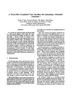
The dissimilarity profiles of both measures are based on three piecewise constant quantities (see Fig. 1A). These are the time of the preceding spike tp共n兲共t兲 ⫽ max共ti共n兲ⱍt共i n兲 ⱕ t兲 t1共n兲 ⱕ t ⱕ t共Mn兲 ,

(2)

n

the time of the following spike tF共n兲共t兲 ⫽ min(ti共n兲|ti共n兲 ⬎ t) t共1 n兲 ⱕ t ⱕ t共Mn兲 ,

(3)

n

as well as the interspike interval (n) xISI 共t兲 ⫽ tF共n兲共t兲 ⫺ tP共n兲共t兲 .

(4)

spike train auxiliary leading spikes at time t ⫽ 0 and auxiliary trailing spikes at time t ⫽ T (but also see The SPIKE-distance). The ISI-distance. The ISI-distance, proposed as a bivariate measure in Kreuz et al. (2007) and extended to the multispike train case in Kreuz et al. (2009), was the first spike train distance directly defined as the temporal average of an instantaneous dissimilarity profile. This profile is calculated as the absolute value of the instantaneous ratio between the interspike (1) (2) intervals xISI and xISI (see Fig. 1A) according to: I共t兲 ⫽

(1) tF

x(1)

ISI

Spike trains (2)

xISI

2 t(2)

t(2)

t

P

F

B (1)

tP

(1)

x(1)

(1)

1

tF

xF

P

(1)

(1)

Δ tP

Spike trains

Δ t(2) P

Δ tF x(2) P

2 (2) P

(2) F

t

t

C 1

t(1)

t(1)

i−1

i

t(1)

i+1

(1) Jij = 0 ti−1

i+1

i

τij

Spike trains

t(1)

t(1)

t(2) j

τij

t(2) j+1

t(2) j−1

t(2) j

T

i

兰

T

0

dtI共t兲 .

(6)

ⱍ

ⱍ兲

(7)

and analogously for tF(1), tP(2), and tF(2) (see Fig. 1B). Subsequently, for each spike train separately, a locally weighted average is employed such that the differences for the closer spike dominate; for each spike train n ⫽ 1, 2 the weighting factors are the intervals to the previous and to the following spikes: xP(n)共t兲 ⫽ t ⫺ tP(n)共t兲

(8)

xF(n)共t兲 ⫽ tF(n)共t兲 ⫺ t.

(9)

and

2 t(2) j−1

1

⌬tP(1)共t兲 ⫽ min共 tP(1)共t兲 ⫺ t(2) i

F

t

Jij = 1

DI ⫽

Δ t(2) F

x(2)

(5)

The SPIKE-distance. The SPIKE-distance (see Kreuz et al. 2011 for the original proposal, and Kreuz et al. 2013 and Kreuz 2012 for the definite version presented here) is the centerpiece of SPIKY. In contrast to the ISI-distance, it considers the exact timing of the spikes. The dissimilarity profile is calculated in two steps: first for each spike a spike time difference is calculated and then for each time instant the relevant spike time differences are selected, weighted, and normalized. Here “relevant” means local; each time instant is surrounded by four corner spikes: the preceding spike from the first spike train tP(1), the following spike from the first spike train tF(1), the preceding spike from the second spike train tP(2), and, finally, the following spike from the second spike train tF(2). To each of these corner spikes one assigns the distance to the nearest spike in the other spike train, for example, for the previous spike of the first spike train:

A 1

(2) 共t兲 ⫺ xISI 共t兲ⱍ (1) (2) max共xISI共t兲, xISI共t兲兲 (1) ISI

Since the ISI-values only change at the times of spikes, the dissimilarity profile is piecewise constant (with discontinuities at the spikes). The ISI-ratio equals zero for identical interspike intervals in the two spike trains and approaches one in intervals in which one spike train is much faster than the other. The ISI-distance is defined as the temporal average of this absolute ISI-ratio:

The ambiguity regarding the definition of the very first and the very last interspike interval is resolved by placing for each

(1) tP

ⱍx

t(2) j+1

Time [arbitrary unit] Fig. 1. A: ISI-distance. Illustration of the local quantities used to define the dissimilarity profile I(t) for an arbitrary time instant t. B: SPIKE-distance. Illustration of the additional local quantities needed for the calculation of the dissimilarity profile S(t). C: SPIKE-synchronization. Illustration of the adaptive coincidence detection (which was originally proposed for event synchronization). While in the first half the middle spikes t(1) and t(2) are coincident, j i the middle spikes in the second half are not.

The local weighting for the spike time differences of the first spike train reads: S 1共 t 兲 ⫽

⌬tP(1)共t兲xF(1)共t兲 ⫹ ⌬tF(1)共t兲xP(1)共t兲 (1) xISI 共t兲

,

(10)

and analogously S2(t) is obtained for the second spike train. Averaging over the two spike train contributions and normalizing by the mean interspike interval yields:

J Neurophysiol • doi:10.1152/jn.00848.2014 • www.jn.org

Innovative Methodology SPIKY

S ⬙共 t 兲 ⫽

S 1共 t 兲 ⫹ S 2共 t 兲 (n) 2具xISI

共t兲 典n

.

(11)

This quantity sums the spike time differences for each spike train weighted according to the relative distance of the corner spike from the time instant under investigation. This way relative distances within each spike train are taken care of, while relative distances between spike trains are not. To get these ratios straight and to account for differences in firing rate, in a last step the two contributions from the two spike trains are locally weighted by their instantaneous interspike intervals. This leads to the definition of the dissimilarity profile: S共t兲 ⫽

(2) (1) S1共t兲xISI 共t兲 ⫹ S2共t兲xISI 共t兲 (n) 2具xISI

共t兲

典2n

.

(12)

Again, the overall distance value is defined as the temporal average of the dissimilarity profile: DS ⫽

兰 T 1

T

0

dtS共t兲 .

(13)

Since the dissimilarity profile S(t) is obtained from a linear interpolation of piecewise constant quantities, it is piecewise linear (with potential discontinuities at the spikes). Both the dissimilarity profile S(t) and the SPIKE-distance DS are bounded in the interval [0, 1]. The distance value DS ⫽ 0 is obtained for identical spike trains only. Due to the finite recording time there is an ambiguity regarding the definitions of the initial distance to the preceding spike, the final distance to the following spike, as well as the very first and the very last interspike intervals. In previous implementations of the SPIKE-distance this ambiguity was resolved by adding to each spike train an auxiliary leading spike at time t ⫽ 0 and an auxiliary trailing spike at time t ⫽ T. This led to spurious synchrony at the edges whereby construction of the dissimilarity profile reached the zero value. Here we partly correct this edge effect by incorporating all the information that is available. We describe the correction only for the beginning of the recording; an analogous procedure is applied at the end of the recording. We count the auxiliary spikes as normal spikes that can be nearest neighbors to other spikes. However, instead of calculating their spike time distance (which is always zero) we use the spike time difference of the first real spike. For the first interspike interval we know that it is at least the distance to the first spike t1 ⫺ t0 ⫽ t1, but it could be longer. Therefore, to take the local firing rate into consideration we set xISI共0兲 ⫽ max共t1, t2 ⫺ t1兲 .

(14)

where we use the length of the first known interspike interval t2 ⫺ t1 as a lower limit. In case t1 is smaller than t2 ⫺ t1 we get at least a crude estimate of how much longer the first interspike interval could have been. Real-time SPIKE-distance. In contrast to the dissimilarity profile S(t) of the regular SPIKE-distance, the dissimilarity profile Sr(t) of the real-time SPIKE-distance can be calculated online because it relies on past information only. From the perspective of an online measure, the information provided by the following spikes, both their position and the length of the interspike interval, is not yet available. Like the profile of the

3435

regular SPIKE-distance, this causal variant is also based on local spike time differences but now only two corner spikes are available, and the spikes of comparison are restricted to past spikes, e.g., for the preceding spike of the first spike train:

ⱍ

⌬tP共1兲共t兲 ⫽ min 共 tP共1兲共t兲 ⫺ t共i 2兲 i:tiⱕt

ⱍ兲 .

(15)

Since there are no following spikes available, there is no local weighting. There is no interspike interval either, so the normalization is achieved by dividing the average corner spike difference by twice the average time interval to the preceding spikes (Eq. 8). This yields a causal indicator of local spike train dissimilarity: Sr(t) ⫽

⌬tP共1兲共t兲 ⫹ ⌬tP共2兲共t兲 4具xP共n兲共t兲 典n

.

(16)

Forward SPIKE-distance. The dissimilarity profile Sf(t) of the forward SPIKE-distance is “inverse” to the profile of the real-time SPIKE-distance. Instead of relying on past information only it relies on forward information only. It can be used in triggered temporal averaging to evaluate the (causal) effect of certain spikes or of specific stimuli features on future spiking. Again, for each time instant there are just two corner spikes and the potential nearest spikes in the other spike train are future spikes only. Thus the spike time difference for the following spike of the first spike train reads:

ⱍ

⌬tF共1兲共t兲 ⫽ min 共 tF共1兲共t兲 ⫺ t共i 2兲 i:tiⱖt

ⱍ兲

(17)

and accordingly for the following spike of the second spike train. In analogy to Eq. 16, an indicator of local spike train dissimilarity is obtained as follows: S f (t) ⫽

⌬tF共1兲共t兲 ⫹ ⌬tF共2兲共t兲 4具xF共n兲共t兲 典n

.

(18)

SPIKE-Synchronization SPIKE-synchronization quantifies the degree of synchrony from the relative number of quasisimultaneous appearances of spikes. Since it builds on the same bivariate and adaptive coincidence detection that was used for event synchronization (Quian Quiroga et al. 2002; see also Kreuz et al. 2007), SPIKE-synchronization is parameter and scale free as well. Coincidence detection typically uses a coincidence window ␶(1,2) , which denotes the time lag below which two spikes from ij two different spike trains, t(1) and t(2) i j , are considered to be coincident. For both event synchronization and SPIKE-synchronization this coincidence window is adapted to the local spike rates (see Fig. 1C): (1) (1) (1) (1) (2) (2) (2) ␶共ij1,2兲 ⫽ min兵ti⫹1 ⫺ t(1) i , ti ⫺ ti⫺1, t j⫹1 ⫺ t j , t j ⫺ t j⫺1其 ⁄ 2. (19)

The coincidence criterion can be quantified by means of a coincidence indicator C共i 1兲 ⫽

再

(2) (1,2) 1 if min j(|t(1) i ⫺ t j |) ⬍ ␶ij

0 otherwise

(20)

[and analogously for C(2) j ] that assigns to each spike either a one or a zero depending on whether it is part of a coincidence or not. The minimum function in Eq. 20 takes already into

J Neurophysiol • doi:10.1152/jn.00848.2014 • www.jn.org

Innovative Methodology 3436

SPIKY

account that a spike can at most be coincident with one spike (the nearest one) in the other spike train. This is a consequence of the adaptive definition of ␶(1,2) in Eq. 19 and the “⬍” in Eq. ij 20 (which has been changed from the “ⱕ” used in the original definition of event synchronization). In case a spike is right in the middle between two spikes from the other spike train there is no ambiguity any more since there is no coincidence. This way we have defined a coincidence indicator for each individual spike of the two spike trains. To obtain one combined similarity profile we pool the spikes of the two spike trains as well as their coincidence indicators by introducing one overall spike index k. In case there exist exact matches (pairs of perfectly coincident spikes) k counts over both spikes. This yields one unified set of coincidence indicators Ck in which according to Eqs. 19 and 20 each coincidence leads to a pair of consecutive ones. From this discrete set of coincidence indicators Ck the SPIKE-synchronization profile C(tk) is obtained via C(tk) ⫽ C(k). Finally, SPIKE-synchronization is defined as the average value of this profile SC ⫽

1

M

兺 C 共 t k兲 M k⫽1

(21)

with M ⫽ M1 ⫹ M2 denoting the total number of spikes in the pooled spike train. The interpretation is very intuitive: SC quantifies the fraction of all spikes in the two spike trains that are coincident. It is zero for spike trains without any coincidences and reaches one if and only if the two spike trains consist only of pairs of coincident spikes. The extension to the case of more than two spike trains (N ⬎ 2) is straightforward. First, bivariate coincidence detection is performed for each pair of spike trains (n, m). Generalizing Eq. 20 gives the coincidence indicators C共i n,m兲 ⫽

再

(m) (n,m) 1 if min j(|t(n) i ⫺ t j |) ⬍ ␶ij

0 otherwise

(22)

where ␶(n,m) is defined as in Eq. 19, but for arbitrary spike trains ij n and m. Subsequently, for each spike of every spike train a normalized coincidence counter C共i n兲 ⫽

1

兺 C共i n,m兲 .

N ⫺ 1 m⫽n

(23)

is obtained by averaging over all N ⫺ 1 bivariate coincidence indicators involving the spike train n. As in the bivariate case, pooling leads to just one set of normalized coincidence counters Ck each of which can obtain any one out of this finite set of values: 0, 1/(N ⫺ 1), . . ., (N ⫺ 1)/ (N ⫺ 1) ⫽ 1. Again, the multivariate SPIKE-synchronization profile C(tk) is obtained via C(tk) ⫽ C(k) and its average value yields the multivariate SPIKE-synchronization SC ⫽

1

M

兺 C 共 t k兲 M k⫽1

(24)

where M ⫽ 冱N n Mn again denotes the overall number of spikes. Note that Eq. 24 is completely analogous to Eq. 21. Moreover, setting n ⫽ 1, m ⫽ 2, and N ⫽ 2 in Eqs. 22 and 23 retrieves Eq. 20. Therefore, the bivariate equations are just a special case of the more general multivariate formulation.

Accordingly, the interpretation of SPIKE synchronization as the overall fraction of coincident spikes is general and holds for both bivariate and multivariate datasets. SPIKE-synchronization is zero if and only if the spike trains do not contain any coincidences and reaches one if and only if each spike in every spike train has one matching spike in all the other spike trains. Examples for both of these extreme cases can be found in Fig. 2, B and D. In contrast to I(t) and S(t), the time-resolved SPIKE-synchronization C(tk) is a measure of similarity. The PSTH is oriented the same way so it makes sense to compare these two measures (Fig. 2). The SPIKE-synchronization profile C(tk) is only defined at the times of the spikes, but a better visualization can be achieved by connecting the individual dots. For larger spike train datasets (here example in Fig. 2A) it also makes sense to smooth the profile with a moving average of appropriate order. Figure 2A demonstrates the similarities and dissimilarities between the PSTH and SPIKE-synchronization on a rather general example. Figure 2, B–D, shows that SPIKEsynchronization, in contrast to the PSTH, is a true measure of spike train synchrony (see also Kreuz 2011). Since the PSTH is invariant to shuffling spikes among the spike trains, it yields the same value regardless of how spikes are distributed among the different spike trains. Comparison with Other Implementations The very first all-in-one implementation of the ISI- and the SPIKE-distance was published online at the time of the publication of Kreuz et al. (2013).1 In between this first and our current release, several other source codes written in various languages and for different platforms have been made available. The most prominent examples are the Python-Implementation of the SPIKE-distance courtesy of Jeremy Fix and available on his homepage and the C⫹⫹-Implementation of both ISI- and SPIKE-distance courtesy of Razvan Florian and hosted on GitHub.2,3 The SPIKE-distance was also implemented in the commercially distributed HRLAnalysis software suite (Thibeault et al. 2014) designed for the analysis of large-scale spiking neural data. Note that all of these implementations are restricted to the dissimilarity profile and its temporal average (the overall dissimilarity). In contrast, SPIKY also allows the user to interactively access all the other different ways to extract information that will be introduced in LEVELS OF INFORMATION EXTRACTION. All of these codes for calculating the ISI- and the SPIKEdistance rely on equidistantly sampled dissimilarity profiles, and the same holds true for codes of event synchronization. Typically, the precision is set to the sampling interval of the neuronal recording. Since the dissimilarity profiles have to be calculated and stored for each pair of spike trains, one obtains, for each measure, a matrix of order “number of time instants” ⫻ “number of spike train pairs” [i.e., #(ts) ⫻ N(N ⫺1)/2]. For small sampling intervals and large numbers of spike trains this leads to memory problems. In SPIKY we use an optimized and more memory-efficient way of storing the results. We make use of the fact that the 1

This section concerns only the ISI- and the SPIKE-distance. Since SPIKEsynchronization is a new proposal there are no other implementations. 2 http://jeremy.fix.free.fr/Softwares/spike.html. 3 https://github.com/modulus-metric/spike-train-metrics.

J Neurophysiol • doi:10.1152/jn.00848.2014 • www.jn.org

Innovative Methodology SPIKY

3437

A Spike trains PSTH 0.1 0

C 0.5 0 0

B

500

1000

1500

2000

2500

3000

3500

4000

Spike trains PSTH 0.2 0

C 0.5

C

0

Spike trains PSTH 0.2 0

C 0.5

D

0

Spike trains

Fig. 2. Comparison of peristimulus time histogram (PSTH) and SPIKE-synchronization. For the latter we added a dashed similarity profile that serves as a visual aid only. A: multivariate example with 50 spike trains. In the first half within the noisy background there are 4 regularly spaced spiking events with increasing jitter. The second half consists of 10 spiking events with decreasing jitter but now without any noisy background. In the noisy first half PSTH and the smoothed SPIKE-synchronization exhibit very similar profiles. The fact that the firing events become more distinct in the second half is indicated by the smoothed SPIKE-synchronization as a gradual increase to synchronization. In the PSTH the peaks become more and more narrow. B–D: by construction the pooled spike train of these examples is identical consisting of 10 evenly spaced bursts. The only difference is the distribution of the spikes among the individual spike trains, which varies from low via intermediate to high synchrony. Whereas the PSTH is the same for all three examples, SPIKE-synchronization correctly indicates the increase in synchrony (note that in B SPIKEsynchronization attains the value zero and in D the value one over the whole time interval, see arrows). B: synfire chain of bursts. C: random distribution of spikes among spike trains. D: high reliability. Each spike train contains 1 spike per firing event.

PSTH 0.2 0

C 0.5 0 0

200

400

600

800

1000

Time dissimilarity profile I(t) of the ISI-distance is piecewise constant and the dissimilarity profile S(t) of the SPIKE-distance is piecewise linear. Each constant/linear interval runs from one spike of the pooled spike train to the next. Thus, for each such interval (and for each pair of spike trains), we have to store only one value for the ISI-dissimilarity and two values for the SPIKE-dissimilarity, one at the beginning and one at the end of the interval (see Fig. 3). The memory gain is proportional to the number of sample points per interspike interval in the pooled spike train and is typically much larger than one. The dissimilarity profiles exhibit instantaneous jumps at the times of the spikes since this is where the lengths of the interspike intervals and the identity of the previous and the following spikes change abruptly or where a new coincidence is counted. For sampled dissimilarity profiles one has to “cut the corners” of these instantaneous jumps. This leads

to an estimation error that increases with the sampling interval. In contrast, within the new implementation each spike marks both the end of the previous and the beginning of the next interval and it becomes possible to store two dissimilarity values for these points. This way the integration from one spike of the pooled spike train to the next can be performed over the full interval. Thus, besides being far more memory efficient, the new implementation also computes the exact distance values without any spurious dependence on the sampling interval. The third effect of the new implementation is a considerable speed-up. To show this (and to provide relative computational costs for the different measures) we here calculate the speed gain achieved by going from the old equidistantly sampled implementation to the new minimally sampled implementation of the ISI- and the SPIKE-distance.

J Neurophysiol • doi:10.1152/jn.00848.2014 • www.jn.org

Innovative Methodology 3438

SPIKY

Spike trains

Pooled Ia 0.4

0 a

S

0.2

0 0

100

200

300

400

500

600

700

800

900

1000

Time Fig. 3. Illustration of the memory efficient storage of the dissimilarity profile for both the ISI- and the SPIKE-distance.

As benchmark we use the comprehensive performance comparison carried out by Rusu and Florian (2014). In this test the authors compared the performance of their newly proposed modulus-metric with the performance of previously proposed spike train distances including the ISI- and the SPIKE-distance. Like them we used two random spike trains with different numbers of spikes. However, since we were also interested in applications to larger datasets, we extended the maximum number of spikes from 500 to 10,000 spikes. The firing rate is kept constant; hence, the duration of the trial increases with the number of spikes. For a fair comparison we implemented all algorithms in C⫹⫹ and ran them on an Intel i7-4700MQ CPU @ 2.4 GHz. All speed gains were averaged over 10,000 trials (Fig. 4). In a first step we replicated the results of Rusu and Florian (2014), who had calculated the ISI- and SPIKE-distances using dissimilarity profiles that were equidistantly sampled with a fixed time step of dt ⫽ 1 ms. Rerunning the same algorithms on our computer, we could reproduce their results (for ⬍500 spikes) within the same order of magnitude. Subsequently, we measured the running times using minimally sampled dissimilarity profiles and found that for both the ISI- and the SPIKEdistance the new implementation was considerably faster than the old implementation. As expected, the speed gain depends critically on the sampling rate used for the old implementation and is particularly large for densely sampled data (Fig. 4). Apart from minimal sampling, SPIKY includes another improvement that strongly increases the overall performance. The source codes published along with Kreuz et al. (2013) were entirely written in Matlab. In contrast, the new SPIKYimplementation uses C-based Matlab executables (MEX)-files for the most time-consuming parts and this leads to another enormous performance boost (typically by a factor between 3 and 30). LEVELS OF INFORMATION EXTRACTION

The ISI- and the SPIKE-distance combine a variety of properties that make them well suited for the application to real data. In particular, they are conceptually simple, computationally efficient, and easy to visualize in a time-resolved manner. By taking into account only the preceding and the following

spike in each spike train, these distances rely on local information only. They are also time-scale adaptive since the information used is not contained within a window of fixed size but rather within a time frame whose size depends on the local rate of each spike train. Moreover, the sensitivity to spike timing and the instantaneous reliability achieved by the SPIKE-distance open up many new possibilities in multineuron spike train analysis (Kreuz et al. 2013). These build on the fact that there are several ways to extract information all of which we describe in the following. As an illustration we use the detailed analysis of an artificially generated spike train dataset with the SPIKEdistance (for the raster plot see Fig. 5A, top). Since the profile of SPIKE-synchronization is only defined at the times of the spikes and not at any instantaneous instants, for this measure only a few of these levels apply, as we will explain in more detail below. Full Matrix and Cross Sections The starting point is the most detailed representation in which one instantaneous value is obtained for each pair of spike trains (see Eq. 12). This representation could be viewed as a movie of a symmetric pairwise dissimilarity matrix in which each frame corresponds to one time instant (an example can be found in the Supplemental Material of Kreuz et al. 2013). For a movie of finite length the time axis necessarily has to be sampled but in principle this most detailed representation consists of an infinite number of values. However, since all dissimilarity profiles are piecewise linear there is a lot of redundancy. One step towards a more compact and memory-efficient representation is to store all pairwise dissimilarity profiles in a matrix of size “number of interspike intervals in the pooled spike train” ⫻ “number of spike train pairs” (⫻2 for the SPIKE-distance, see Comparison with Other Implementations). From this two-dimensional matrix it is possible to extract both kinds of cross sections. By selecting a pair of spike trains, one obtains the bivariate dissimilarity profile S(t) for this pair of spike trains. Selecting a time instant ts (and using linear interpolation for time instants in between spikes) yields an instantaneous matrix of pairwise spike train dissimilarities Smn(ts) (see Fig. 5B). This matrix can be used to divide the spike trains into instantaneous clusters, that is, groups of spike trains with low intragroup and high intergroup dissimilarity. For SPIKE-synchronization it is possible to select pairwise dissimilarity profiles but instantaneous matrices are not defined. Spatial and Temporal Averaging Another way to reduce the information of the dissimilarity matrix is averaging. There are two possibilities that commute: the spatial average over spike train pairs and the temporal average. Since the spatial average over spike train pairs can be done locally, it yields a dissimilarity profile for the whole population. Examples for averages over four different spike train groups as well as over all spike trains are shown in Fig. 5A, bottom. Temporal averaging over certain intervals on the other hand leads to a bivariate distance matrix (see Fig. 5, C and D, for examples of noncontinuous and continuous intervals). In real data, these temporal intervals could be chosen to

J Neurophysiol • doi:10.1152/jn.00848.2014 • www.jn.org

Innovative Methodology SPIKY

B

400

800

300

600

Speed gain

Speed gain

A

3439

200 100

Fig. 4. Speed gain achieved by the new (minimally sampled) implementation of ISI-distance (A) and SPIKE-distance (B) with respect to the old (equidistantly sampled) implementation in dependence on the number of spikes and on the time step used by the old implementation.

400 200

0 0.01

0 0.01

10000

10000

Ti

0.1

m

e

1000 100

st

ep

1 10

Nu

mb

e

f ro

ke spi

Ti

s

0.1

m

e

1000 100

st

ep

1 10

correspond to different external conditions such as normal vs. pathological, asleep vs. awake, target vs. nontarget stimulus, or presence/absence of a certain channel blocker. A combination of temporal and spatial averaging can be seen in Fig. 5F. This dissimilarity matrix is obtained from the

Nu

mb

e

fs ro

pik

es

overall temporal average shown in Fig. 5D by (spatially) averaging over the 16 submatrices and thus depicts the pairwise spike train group dissimilarity (4 ⫻ 4 instead of 20 ⫻ 20). Figure 5G shows the respective dendrogram. In applications to real data, these groups could be different neuronal populations

1

A

2 3

4

G1 G2 G3 G4 0.4

0.192

Sa

0 0

200

400

600

800

1000

1200

1400

1600

1800

2000

Time

1

Spike trains

B

2

C

3

D

4

E

1

5 10

0.5

15 20 5

10

15

20

5

Spike train groups

Spike trains

F

10

15

20

Spike trains

10

15

20

5

Spike trains

G

G1

5

H

10

15

20

0

Spike trains

I

G2 G3 G4 G1

G2

G3

G4

Spike train groups

1

2

3

4

Spike train groups

Spike trains

Spike trains

J Neurophysiol • doi:10.1152/jn.00848.2014 • www.jn.org

Fig. 5. The different levels of information extraction for the SPIKE-distance. A, top: spike raster plot of 20 artificially generated spike trains divided in 4 spike train groups of 5 spike trains each. The clustering behavior changes every 500 ms. A, bottom: dissimilarity profiles of the SPIKE-distance for the 4 spike train groups (thin color-coded lines) and for all spike trains (thick black line). The overall dissimilarity is defined as the temporal average of the dissimilarity profile of all spike trains (0.192 in this case) and is marked by a dashed horizontal line. The green lines and symbols on top of the raster plot mark temporal instants and intervals results of that are detailed in the subplots at the bottom. B–E: matrices of pairwise instantaneous dissimilarity values for a single time instant (B, mark 1), for 2 selective averages (over nonconsecutive intervals in C, mark 2, and over the whole interval in D, mark 3), and for a triggered average (E, mark 4). F and G: for the overall average (mark 3) we also show the matrices of overall pairwise instantaneous dissimilarity values for the 4 spike train groups (F) and the corresponding dendrogram (G). H and I: dendrogram of spike train matrices in D and E. Note that in contrast to the overall average (mark 3 shown in H) the triggered average (mark 4 shown in I) captures the local similarity between 5 of the spike trains.

Innovative Methodology 3440

SPIKY

or responses to different stimuli, depending on whether the spike trains were recorded simultaneously or successively. Finally, successive application of spatial average over all spike train pairs and temporal average over the whole interval results in just one distance value that describes the overall level of dissimilarity for the entire dataset. In Fig. 5A this value is stated in the bottom top right. Both spatial and temporal averaging are well-defined for SPIKE-synchronization and so is the overall value. Triggered Averaging The fact that there are no limits to the temporal resolution allows further analyses such as internally or externally triggered temporal averaging. Here, the matrices are averaged over certain trigger time instants only. The idea is to check whether this triggered temporal average is significantly different from the global average since this would indicate that something peculiar is happening at these trigger instants. The trigger times can either be obtained from external influences (such as the occurrence of certain features in a stimulus) or from internal conditions (such as the spike times of a certain spike train). External triggering is a standard tool to address questions of neural coding, for example, it can be used to evaluate the influence of localized stimulus features on the reliability of neurons under repeated stimulation. In multineuron data, internal triggering might help to uncover the connectivity in neural networks or to detect converging or diverging patterns of firing propagation. An example is shown in Fig. 5E. Here, neurons 2, 9, 14, and 19 follow the 7th neuron during the 2nd and the 4th 500-ms subinterval. This can be revealed by triggering on the spike times of neuron 7 during these subintervals. The difference between the dissimilarity matrix of the full interval in Fig. 5D and the triggered dissimilarity matrix of Fig. 5E can be best seen by comparing the respective dendrograms in Fig. 5, H and I. Since instantaneous values are not defined, triggered averaging does not make any sense for SPIKE-synchronization. SPIKY

SPIKY is a graphical user interface for monitoring synchrony between artificially simulated or experimentally recorded neuronal spike trains. It contains implementations of the ISI-distance, the SPIKE-distance, and SPIKE-synchronization. Moreover, SPIKY includes the forward variant of the SPIKE-distance as well as a “simulation” of the real-time SPIKE-distance. The latter calculates the values the real-time version would give but instead of going forward in real time it just calculates all values in parallel (see also Outlook). The source codes are written in Matlab (MathWorks, Natick, MA) with the most time-consuming loops coded in MEX-files.4 Consequently, SPIKY is not stand-alone but requires Matlab to run. The following sections give a broad overview of the features of SPIKY. For a more detailed description of the specific procedures that realize these features please refer to the documentation and the web pages listed below. 4 In our case these are subroutines written in C. However, as some users may not have access to a suitable C compiler, SPIKY contains the (slower) pure Matlab code as well.

Access to SPIKY and How to Get Started SPIKY is distributed under the BSD license [Copyright (c) 2014, Thomas Kreuz, Nebojsa Bozanic. All rights reserved]. A zip-package containing all the necessary files can be accessed for free on the download page.5 This package also contains a folder with documentation (such as a FAQ-file and an introduction to all individual elements of SPIKY and all individual files of the SPIKY-package). Further information and many demonstrations (both images and movies) can be found on the download page and on the SPIKY Facebook page.6 Both of these pages are used to announce updates and distribute the latest information about new features. They also provide an opportunity to give feedback and ask questions. Moreover, the Facebook page includes various screen recordings with voiceover in which the user is guided step by step through some of the most important features of SPIKY. All of these movies can also be viewed on the SPIKY YouTube channel.7 After downloading SPIKY the user has to first extract the zip-package, which leaves all files in one folder named “SPIKY.” If the system has a suitable MEX-compiler installed, the MEX-files can be compiled from within this folder by running the m-file “SPIKY_compile_MEX.” The program is started with the m-file “SPIKY.” When SPIKY is running, the user has the option to select to view short hints (“tooltips”) when hovering above individual elements of the graphical user interface. An overview of all the information contained in the hints can be found in the documentation file “SPIKY-Elements.” Furthermore, at each step the suggested element for the next user action is highlighted by a bold font. To get the user started quickly, SPIKY provides a few example datasets from previous publications. The most useful example is the “Clustering” dataset, which has already been used in several figures as well as in the Supplemental Movie of Kreuz et al. (2013). The best way to get acquainted with SPIKY is to advance from panel to panel by pressing the highlighted button. When the end is reached the user can reset and run the same example again while changing some parameters to see the consequences. Note that it is not necessary to set all the parameters each time when SPIKY is started. Rather, it is possible to use the file “SPIKY_f_user_interface” to set and modify the spike train data as well as the parameters (again, the dataset “Clustering” provides an example). Structure and Workflow of SPIKY Overall, SPIKY has a rather linear workflow; however, it is much more interactive than previous implementations of the measures and there are many potential shortcuts and loops along the way. As can be seen in the SPIKY-flowchart in Fig. 6, the general flow is clearly directed from the input of spike train data to the output of results. Therefore, the first step the user has to do is to give SPIKY spike train data (i.e., sequences of spike times) to work with. There are four possible ways to do this: one can make use of predefined examples, load data from a file or from the Matlab workspace, detect discrete events from continuous data, or employ the spike train generator (see Input for more details on the SPIKY input). 5 6 7

http://www.fi.isc.cnr.it/users/thomas.kreuz/Source-Code/SPIKY.html. https://www.facebook.com/SPIKYgui. https://www.youtube.com/user/SPIKYgui1.

J Neurophysiol • doi:10.1152/jn.00848.2014 • www.jn.org

Innovative Methodology SPIKY Event detector

Load data

MODIFY DATA

GET DATA

Update

Spike train generator

Use Matlab code

SELECT MEASURES

Reset

Print

Save to file

GET RESULTS Movie

SP KY SELECT TIME INSTANTS/AVERAGES

Export variables

Calculate

Plot MODIFY PLOTS

SELECT PLOTS Plot

Fig. 6. SPIKY-logo (center) and flowchart describing the workflow of SPIKY from the input of spike train data to the output of results. A typical SPIKYsession begins at the top with “Get data” and then goes clockwise and ends on the left with “Get results.” For clarity we omitted 2 possible actions that can be performed from multiple positions on the workflow circle: From any point it is possible to reset to the very beginning (“reset” leads to the symbol ), and from any later point it is possible to jump back before the measure calculation (“reset with the same data” leads to the symbol p).

Once the full dataset is available, modification is still possible. The user can restrict the analysis to a specific subset, e.g., select a smaller time window and/or a subset of spike trains. It is also possible to impose some external structure on the raster plot (spike trains vs. time). For that, SPIKY allows the definition of two types of time markers (e.g., thick/thin markers for specific events such as seizure onset/offset in epilepsy, trigger onset/offset during stimulation etc.) and two types of spike

A

Separators2

Separators1

Spike train group separators

3441

train separators (e.g., a thick separator for neurons from the left vs. neurons from the right hemisphere and a thin separator for different regions within the two halves). The user can also define spike train groups. Depending on the setup these could be spike trains recorded in different brain regions or upon presentation of different stimuli. Figure 7 shows an example of a raster plot with annotations marking all these different elements. After updating all of these data parameters, the next step is to select the measures to be calculated. Options include the PSTH as well as all measures described in detail in MEASURES AND IMPLEMENTATION. In the same step the user can select successive frames for a temporal analysis of spike train patterns. These can be individual time instants for cross sections, temporal intervals for selective averages, and sequences of time instants for triggered averages (see LEVELS OF INFORMATION EXTRACTION). Now the actual calculation of the measures takes place. For reasonably sized datasets this should take at most a few seconds. Very large datasets (typically datasets containing hundreds of spike trains and/or hundred thousands of spikes) are divided in smaller subintervals and the calculation will be performed in a loop that might take longer. It is from this point on that SPIKY becomes truly interactive. Now the user can switch between different representations of the results (such as dissimilarity profiles, dissimilarity matrices, and dendrograms). Different matrices and dendrograms can be compared in the same figure or they can be viewed in sequence. The presentation can be restricted to smaller time windows and/or subsets of spike trains, and temporal and spatial averaging (for example moving average and average over spike train groups) can be performed. Spike trains or spike train groups can also be sorted according to the number of spikes (either within the whole spike train or within a certain interval) or according to the spike latency with respect to a specific time

Markers1

Markers2

G1 10 G2 20 G3 30 G4 40

Spike trains

B

0 500 1000 Spike train groups (color−coded)

1500

2000 Time [ms]

Sr

S 10

2500

< S >G

3500

20

20

30

30 10 20 30 Spike trains

Spike trains

40

10 20 30 Spike trains

Spike trains

40

4000

< Sr >G

G1

G1

G2

G2

G3

G3

0.4

10

G4

C

3000

0.2

G4 G1 G2 G3 G4 Spike trains

G1 G2 G3 G4 Spike trains

1 4 2 3 Spike train groups

2 3 1 4 Spike train groups

0

J Neurophysiol • doi:10.1152/jn.00848.2014 • www.jn.org

Fig. 7. Annotated screenshot from a movie. A: artificially generated spike trains. B: dissimilarity matrices obtained by averaging over 2 separate time intervals for both the regular and the real-time SPIKE-distance as well as their averages over subgroups of spike trains (denoted by ⬍ · ⬎G). C: corresponding dendrograms.

Innovative Methodology 3442

SPIKY

instant. The order can even depend on the result of the clustering analysis, i.e., spike trains belonging to the same cluster will appear next to each other. Furthermore, it is possible to add further figure elements such as spike number histograms, overall averages, or dissimilarity profiles for individual spike train groups. At this stage the user can also retrospectively change the appearance of all the individual elements of the figure (see Figure layout for more details). Finally, SPIKY allows the user to extract both data and results to the Matlab workspace for further analysis, and it is also possible to save individual figures as postscript file or a sequence of figures as an “avi”-movie (see Output for more details on the SPIKY output). Input. There are four different ways to input spike train data into SPIKY. The first option is to select one of the predefined examples that are generated using Matlab-code. Initially these are the examples used in Kreuz et al. (2013) but one can also define new examples. The second option is to load spike train data either from the Matlab workspace or from a file. Two different file formats are accepted, “.mat” and “.txt” (ASCII) files. For the mat-files SPIKY currently allows three different kinds of input formats (further formats can be added on demand): 1) Cell arrays (ca) with just the spike times. This is the preferred format used by SPIKY since it is most memory efficient. The two other formats will internally be converted into this format; 2) Rectangular matrices with each row being a spike train and zero padding (zp) in case of nonidentical spike numbers; and 3) Matrices representing time bins where each zero/one (01) indicates the absence/presence of a spike. In case of a mat-file or of the workspace, SPIKY looks for a variable called “spikes”; if it cannot find it, the user has the chance to select the variable name (or field name) that contains the spikes via an input mask that provides a hierarchical structure tree of all the variables and fields contained in the mat-file or in the workspace. In the text format spike times should be written as a matrix with each row being one spike train. The SPIKY-package contains one example file for all four formats (“testdata ca.mat,” “testdata zp.mat,” “testdata 01.mat,” and “testdata. txt”). The third option is to use the event detector to detect discrete events in continuous data. There are many different possibilities of defining an event. A variety of standard events (such as local maxima and minima and threshold crossings) with a number of parameters are already included. The fourth option is to create new spike train data via the spike train generator. After setting some defining variables (number of spike trains, start and end time, and sampling interval) the user can build spike trains from predefined spike train patterns (such as periodic, splay, uniform, or Poisson) and/or by manually adding, shifting, and deleting individual spikes or groups of spikes. Figure layout. SPIKY is designed so that it can directly generate figures suitable for publication. The user is given control over the appearance of every individual element (e.g., fonts, lines, etc.) in each type of figure. There are two ways to determine essential properties such as color, font size, or line width. It is possible to change elements in the active figure

while the program is already running. Context menus let the user edit the properties of individual elements or of all elements of a certain type. Conveniently, one can also use the file “SPIKY_f_user_interface” to define the standard values for all the parameters that describe the principal layout of the figure. If a figure contains more than one subplot (besides the subplot containing the spike rasterplot and/or the dissimilarity profiles, these are typically subplots with dissimilarity matrices and dendrograms), it is possible to change their position and size. One can edit all position variables together or change the x-position, the y-position, the width, and the height individually. In case there are several dissimilarity matrices/dendrograms this can be done either for an individual matrix/dendrogram or for all of them at once. Output. From within SPIKY it is possible to extract the spike trains and the results of the analysis (measure profiles, matrices, dendrograms) to the Matlab workspace for further processing. Results will be stored in variables such as “SPIKY_spikes,” “SPIKY_profile_X_1,” “SPIKY_profile_Y_1,” “SPIKY_profilename_1,” “SPIKY_matrix_1,” and “SPIKY_matrix_name_1”. In addition, the results obtained during an analysis will automatically be stored in the output structure “SPIKY_results,” which will have one field for each measure selected. Depending on the parameter selection within SPIKY, for each measure the structure can contain the following subfields that correspond to the different representations identified in LEVELS OF INFORMATION EXTRACTION: 1) SPIKY_results.⬍Measure⬎.name: name of selected measure. 2) SPIKY_results.⬍Measure⬎.overall: level of distance/ synchronization over all spike trains and the whole interval. This is just one value, obtained by averaging over both spike trains and time. 3) SPIKY_results.⬍Measure⬎.matrix: pairwise distance/ synchronization matrices, obtained by averaging over time. 4) SPIKY_results.⬍Measure⬎.time: time-values of overall (dis)similarity profile. 5) SPIKY_results.⬍Measure⬎.profile: overall (dis)similarity profile obtained by averaging over spike train pairs. Note that the dissimilarity profiles are not equidistantly sampled. Rather they are stored as memory efficiently as possible, which means just one value for each interval of the pooled spike train for the ISI- and two values for the SPIKE-distance. Since this format can be more difficult to process, SPIKY includes three functions: “SPIKY_f_selective averaging” for computing the selective average over time intervals, “SPIKY_f_triggered averaging” for calculating the triggered average over time instants, and “SPIKY_f_average_pi” for averaging over many dissimilarity profiles. Furthermore, for the ISIdistance the function “SPIKY_f_pico” can be used to obtain the average value as well as the x- and y-vectors for plotting. Besides the standard way to work with Matlab-figures SPIKY also offers the opportunity to save each figure as a postscript file. Finally, it is possible to save a sequence of figures as an “avi”-movie. GUI vs. Loop SPIKY was mainly designed to facilitate the detailed analysis of one dataset. It enables the user to switch between different representations (see LEVELS OF INFORMATION EXTRAC-

J Neurophysiol • doi:10.1152/jn.00848.2014 • www.jn.org

Innovative Methodology SPIKY TION)

and to zoom in on both spatial and temporal features of interest. However, SPIKY is less convenient for the analysis of many different datasets when, e.g., the statistics of a certain quantity such as an average over a specific time interval should be evaluated over all available datasets (e.g., over all trials of a stimulus setup or for recordings of all subjects, etc.) in some kind of loop. For these purposes the SPIKY-package contains a program called SPIKY_loop, which is complementary to SPIKY. It is not a graphical user interface but it should be simple enough (and plenty of examples are provided) to allow everyone to run the same kind of analysis for many different datasets and to evaluate and compare their “SPIKY_results.” SPIKY_loop provides the full functionality of SPIKY and gives access to time instants and selective and triggered averages as well as averages over spike train groups. Therefore, by combining these two programs it is possible to first use SPIKY for a rather exploratory but detailed analysis of a limited number of individual datasets and then use SPIKY_loop and its output structure “SPIKY_loop_results” to verify whether any effect discovered on the example dataset is consistently present within all of the datasets. Both SPIKY and SPIKY_loop require the storage of matrices of the order “number of interspike intervals in the pooled spike train” ⫻ “number of spike train pairs.” For very large datasets with many spike trains and/or spikes this can lead to memory problems. We addressed this issue by making the calculation sequential, i.e., by cutting the recording interval into smaller segments, and performing the averaging over all pairs of spike trains for each segment separately. In the end the dissimilarity profiles for the different segments (already averaged over pairs of spike trains) are concatenated, and its temporal average yields the distance value for the whole recording interval. During this sequential calculation SPIKY uses a waitbar (which displays the percent completed) to continuously inform the user about the progress. This way, by trading memory against speed, running more loops with smaller matrices takes longer, SPIKY is able to deal with datasets containing more than one hundred spike trains and overall more than one million spikes. Spike Train Surrogates and Significance

A very important issue that has not yet been addressed is statistical significance. Given a certain value of the SPIKEdistance how can one judge whether it reflects a significant decrease or increase in spike train synchrony and does not just lie within the range of values obtained for random fluctuations? One answer to this question is the use of spike train surrogates (Kass et al. 2005; Grün 2009; Louis et al. 2010). The idea is to compare the results for the original dataset with the results obtained for spike train surrogates generated from that dataset. If the value obtained for the original lies outside the range of values for the surrogates, this value can be assumed to be significant to a level defined by the number of surrogates, used (e.g., ␣ ⫽ 0.05 for 19 surrogates or ␣ ⫽ 0.001 for 999 surrogates). The SPIKY-package contains a program “Spiky_loop_ surro,” which was designed to evaluate significance. So far it includes four different types of spike train surrogates. They differ in the properties that are preserved and maintain either the individual spike numbers (obtained by shuffling the

3443

spikes), the individual interspike interval distribution (obtained by shuffling the interspike intervals), the pooled spike train (obtained by shuffling spikes among the spike trains), or the PSTH. In the last case the spike train surrogates are obtained by means of inverse transform sampling, i.e., by resampling from the PSTH using its cumulative distribution function (Ross 1997). Other ways to calculate rate functions (e.g., based on kernels with different bandwidths) will be added in future releases. DISCUSSION

Summary In this article we presented SPIKY, a graphical user interface which facilitates the application of methods of spike train analysis to both simulated and real datasets. Apart from the standard PSTH, SPIKY contains three parameter-free and time-resolved measures (see LEVELS OF INFORMATION EXTRACTION). These measures are complementary to each other since each one addresses a different specific aspect of spike train similarity. While the ISI-distance quantifies local dissimilarities based on covariances of the neurons firing rate profiles, both the SPIKE-distance and SPIKE-synchronization capture the relative timing of local spikes.8 However, whereas the SPIKE-distance weights and normalizes the differences between nearest neighbor spikes, SPIKE-synchronization acts as a binary coincidence detector, i.e., there is a cutoff at the (adaptive) time lag relative to which two neighboring spikes are either considered coincident or not and all detailed information both within or outside this coincidence window is discarded. All of these measures yield instantaneous values for each pair of spike trains, and thus there are many different possible representations of the results (see LEVELS OF INFORMATION EXTRACTION). Often the most informative representation might depend on the amount and type of spike train data and SPIKY can be used to reveal it via some explorative and interactive analysis. SPIKY also allows to alter a given dataset before or after the actual analysis, e.g., to interactively select subintervals or spike train subsets, to define time markers and spike train separators, and to divide the dataset into different spike train groups. In addition to the main GUI designed for the detailed analysis of one dataset, the SPIKY-package also includes two complementary programs. While SPIKY_loop aims at the grand average analysis of large numbers of datasets, SPIKY_ loop_surro allows the estimation of significance levels. In all of these programs we use MEX-files, i.e., C-based Matlab executables for the more time-consuming parts and we exploit the piecewise linearity of the dissimilarity profiles, thereby guaranteeing high computation speed and memory efficiency. Outlook One of the measures included in SPIKY is the real-time SPIKE-distance. The present algorithm calculates its instanta8 One should be aware that all of these measures are based on some explicit notion of localness and simultaneousness and thus they all can be fooled by phase lags, no matter whether these are caused by internal delay loops in one spike train or by a common driver that forces the two time series with different delays. Therefore, any such phase lags should be removed by suitably shifting the time series in a preprocessing step.

J Neurophysiol • doi:10.1152/jn.00848.2014 • www.jn.org

Innovative Methodology 3444

SPIKY

neous dissimilarity values by making use of past information only, but it does so in a speed-optimized and parallelized manner that would not be compatible with an actual real-time implementation. However, such a real-time implementation should actually be simpler and computationally (speed and memory) less problematic even for large numbers of neurons since the only information that would have to be stored at each time instant are the time stamps of the latest spikes of each spike train and their nearest neighbors in the other spike trains. SPIKY was primarily designed to analyze neuronal spike trains. However, in principle it is also applicable to any other kind of discrete data that comes in the form of sequences of time stamps (such as times of bouncing basketballs or timecoded social interactions in a psychological test). Furthermore, in Kreuz et al. (2013) the SPIKE-distance was already applied not only to discrete data but also to an example of continuous data (EEG). To clear the way for such applications SPIKY includes an event detector that allows to bridge the gap between continuous data and our methods for discrete data. We chose to write SPIKY in Matlab due to its popularity in the neuroscience community, ease of use, and the engaging visualization capabilities of its GUI design. Because of its high level parallelization, Matlab provides a powerful tool for processing vectorized data, but it also includes a well-developed MEX-interface for integrating C functions for performance enhancements. C functions do not only lead to an increase in performance, they can also easily be incorporated into other programming platforms. Indeed, we have already ported all four measures (the PSTH, the ISI-distance, the SPIKE-distance, and SPIKE-synchronization) as well as some of the additional SPIKY-functionality to Python as part of the PySpike module, an open-source project hosted on Github.9 As in SPIKY, in PySpike the computation intensive functions are implemented as C backends. Another potential direction would be the extension of the methods used here from the quantification of synchrony within one population of two or more neurons to the quantification of synchrony between two (or more) neuronal populations. Similar extensions have been done for two other spike train distances (Aronov 2003; Houghton and Sen 2008), but both of these methods depend on not one but two parameters. Therefore, one particular challenge for a potential extension of our methods would be to make them parameter-free while maintaining their high temporal resolution. There are still many open questions regarding neuronal synchrony. Among these questions are its role in dynamical diseases like epilepsy and its relevance for neural coding. While a thorough discussion of these issues is beyond the scope of this article, we argue that SPIKY will be a very useful tool for investigation. If epileptic seizures and/or time-dependent stimulations lead to changes in spike train synchrony or spike train clustering, SPIKY should be able to detect them. ACKNOWLEDGMENTS T. Kreuz thanks Marcus Kaiser and his group for hosting him at the University of Newcastle, UK. N. Bozanic thanks John van Opstal and his group for hosting him at the Radboud University, Nijmegen, The Netherlands as well as Joshua D. Berke and his group for hosting him at the University of Michigan, Ann Arbor, MI. We thank Ralph Andrzejak, David Angulo Garcia, 9

https://github.com/mariomulansky/PySpike.

Francesco Battaglia, Roman Bauer, Joshua D. Berke, Paolo Bonifazi, Emily Caporello, Daniel Chicharro, Michael Farries, Tim Gentner, Bon-Mi Gu, Arif Hamid, Conor Houghton, Marcus Kaiser, Jutta Kretzberg, Tatjana Loncar Turukalo, Stefano Luccioli, Jason MacLean, Gorana Mijatovic, Ali Mohebi, Florian Mormann, Leon Paz, Jeffrey Pettibone, Friederice Pirschel, Andreea Sburlea, Peter Taylor, Richard Tomsett, Alessandro Torcini, Jonathan Victor, and Yujiang Wang for useful discussions. We also thank Thomas Alderson, Mayte Bonilla Quintana, Hamid Charkhkar, Didier Desaintjan, Mario DiPoppa, Andres Espinal Jiménez, Mahboubeh Etemadi, Gabriel Chew Guojun, Taekyung Kang, Marion Najac, Oren, Robert Rein, Rodrigo Salazar, Andreea Sburlea, Michael Schaub, Eitan Schechtman, Jannetta Steyn, Matthew Williams, Yunguo Yu, Maja Zorovic for user feedback and Black Square, Conor Houghton, Eugenio Piasini, Matthew Phillips, and Sid Visser for advice. Finally, we thank Daniel Chicharro, Conor Houghton, and Andreea Sburlea for carefully reading the manuscript.

GRANTS T. Kreuz acknowledges the Italian Ministry of Foreign Affairs regarding the activity of the Joint Italian-Israeli Laboratory on Neuroscience and N. Bozanic acknowledges the Serbian Ministry of Youth and Sports. T. Kreuz, M. Mulansky, and N. Bozanic acknowledge funding support from the European Commission through the Marie Curie Initial Training Network “Neural Engineering Transformative Technologies (NETT)” Project 289146, and T. Kreuz was also supported through the European Joint Doctorate “Complex Oscillatory Systems: Modeling and Analysis (COSMOS)” Project 642563.

DISCLOSURES No conflicts of interest, financial or otherwise, are declared by the author(s).

AUTHOR CONTRIBUTIONS Author contributions: T.K., M.M., and N.B. conception and design of research; T.K., M.M., and N.B. performed experiments; T.K., M.M., and N.B. analyzed data; T.K., M.M., and N.B. interpreted results of experiments; T.K., M.M., and N.B. prepared figures; T.K., M.M., and N.B. drafted manuscript; T.K., M.M., and N.B. edited and revised manuscript; T.K., M.M., and N.B. approved final version of manuscript.

REFERENCES Aronov D, Reich DS, Mechler F, Victor JD. Neural coding of spatial phase in V1 of the macaque monkey. J Neurophysiol 89: 3304 –3302, 2003. Bower MR, Stead M, Meyer FB, Marsh WR, Worrell GA. Spatiotemporal neuronal correlates of seizure generation in focal epilepsy. Epilepsia 53: 807– 816, 2012. DiPoppa M, Gutkin BS. Correlations in background activity control persistent state stability and allow execution of working memory tasks. Front Comp Neurosci 7: 139, 2013. Grün S. Data-driven significance estimation for precise spike correlation. J Neurophysiol 101: 1126 –1140, 2009. Hochberg LR, Serruya MD, Friehs GM, Mukand JA, Saleh M, Caplan AH, Branner A, Chen D, Penn RD, Donoghue JP. Neuronal ensemble control of prosthetic devices by a human with tetraplegia. Nature 442: 164 –171, 2006. Houghton C, Sen K. A new multineuron spike train metric. Neural Comput 20: 1495–1511, 2008. Kass RS, Ventura V, Brown EN. Statistical issues in the analysis of neuronal data. J Neurophysiol 94: 8 –25, 2005. Kreuz T, Haas JS, Morelli A, Abarbanel HD, Politi A. Measuring spike train synchrony. J Neurosci Methods 165: 151–161, 2007. Kreuz T, Chicharro D, Andrzejak RG, Haas JS, Abarbanel HD. Measuring multiple spike train synchrony. J Neurosci Methods 183: 287–299, 2009. Kreuz T, Chicharro D, Greschner M, Andrzejak RG. Time-resolved and time-scale adaptive measures of spike train synchrony. J Neurosci Methods 195: 92–106, 2011. Kreuz T. Measures of spike train synchrony. Scholarpedia 6: 11934, 2011. Kreuz T. SPIKE-distance. Scholarpedia 7: 30652, 2012. Kreuz T, Chicharro D, Houghton C, Andrzejak RG, Mormann F. Monitoring spike train synchrony. J Neurophysiol 109: 1457, 2013.

J Neurophysiol • doi:10.1152/jn.00848.2014 • www.jn.org

Innovative Methodology SPIKY Kumar A, Rotter S, Aertsen A. Spiking activity propagation in neuronal networks: reconciling different perspectives on neural coding. Nat Rev Neurosci 11: 615– 627, 2010. Louis S, Gerstein GL, Grün S, Diesmann M. Surrogate spike train generation through dithering in operational time. Front Comp Neurosci 4: 127, 2010. Mainen Z, Sejnowski TJ. Reliability of spike timing in neocortical neurons. Science 268: 1503–1506, 1995. Miller EK, Wilson MA. All my circuits: using multiple electrodes to understand functioning neural networks. Neuron 60: 483– 488, 2008. Mormann F, Andrzejak RG, Elger CE, Lehnertz K. Seizure prediction: the long and winding road. Brain 130: 314 –333, 2007. Nirenberg S, Victor JD. Analyzing the activity of large populations of neurons: how tractable is the problem? Curr Opin Neurobiol 17: 397– 400, 2007. Papoutsi A, Sidiropoulou K, Cutsuridis V, Poirazi P. Induction and modulation of persistent activity in a layer v pfc microcircuit model. Front Neural Circuits 7: 161, 2013. Quian Quiroga R, Kreuz T, Grassberger P. Event synchronization: a simple and fast method to measure synchronicity and time delay patterns. Phys Rev E Stat Nonlin Soft Matter Phys 66: 041904, 2002.

3445

Quian Quiroga R, Panzeri S (Editors). Principles of Neural Coding. Boca Raton, FL: CRC Taylor and Francis, 2013. Ross SM. Introduction to Probability Models (6th ed.). New York: Academic, 1997. Rusu CV, Florian RV. A new class of metrics for spike trains. Neural Comput 26: 306 –348, 2014. Sacré P, Sepulchre R. Sensitivity analysis of oscillator models in the space of phase-response curves: oscillators as open systems. IEEE Control Systems 34: 5074, 2014. Sanchez JC, Principe JC, Nishida T, Bashirullah R, Harris JG, Fortes JA. Technology and signal processing for brain-machine interfaces. IEEE Signal Process 25: 29 – 40, 2008. Shlens J, Rieke F, Chichilnisky EJ. Synchronized firing in the retina. Curr Opin Neurobiol 18: 396 – 402, 2008. Thibeault CM, O’Brien MJ, Srinivasa N. Analyzing large-scale spiking neural data with HRLAnalysis. Front Neuroinform 8: 17, 2014. Tiesinga PH, Fellous JM, Sejnowski TJ. Regulation of spike timing in visual cortical circuits. Nat Rev Neurosci 9: 97–107, 2008. Truccolo W, Donoghue JP, Hochberg LR, Eskandar EN, Madsen JR, Anderson WS, Brown EN, Halgren E, Cash SS. Single-neuron dynamics in human focal epilepsy. Nat Neurosci 14: 635– 641, 2011. Victor JD. Spike train metrics. Curr Opin Neurobiol 15: 585–592, 2005.

J Neurophysiol • doi:10.1152/jn.00848.2014 • www.jn.org