Author manuscript, published in "Graphical Models 65, 1-3 (2003) 149-167" DOI : 10.1016/S1524-0703(03)00009-2
Split and Merge Algorithms Defined on Topological Maps for 3D Image Segmentation Guillaume Damiand a,∗, Patrick Resch b a IRCOM-SIC,
bˆ at SP2MI, BP 30179, 86962 Futuroscope Chasseneuil Cedex, France
b LIRMM,
161 rue Ada, 34392 Montpellier Cedex 5, France
hal-00211741, version 1 - 21 Jan 2008
Abstract Split-and-merge algorithms define a class of image segmentation methods. Topological maps are a mathematical model that represents image subdivisions in 2D and 3D. This paper discusses a split-and-merge method for 3D image data based on the topological map model. This model allows representations of states of segmentations and of merge and split operations. Indeed, it can be used as data structure for dynamic changes of segmentation. The paper details such an algorithmic approach and analyzes its time complexity. A general introduction into combinatorial and topological maps is given to support the understanding of the proposed algorithms. Key words: topological maps, split-and-merge, image segmentation, image processing
1
Introduction
The region segmentation was studied in many different works in 2 dimensions. It consists in making a partition of an image into connected sets of pixels which verify an homogeneity criterion, and which are called regions. A classical approach to region segmentation is the split-and-merge method and all its variants. The top-down approach [22,25] consists in taking big regions and cutting them into smaller and smaller regions. The bottom-up approach [7,16] is the opposite one. It begins with many small regions that are progressively ∗ Corresponding author. Email addresses:
[email protected] (Guillaume Damiand),
[email protected] (Patrick Resch).
Article published in Graphical Models-65(1-3)-pp. 149-167 - May 2003
merged into bigger and bigger regions. At last the mixed approach [18,26] consists in combining the two previous ones.
hal-00211741, version 1 - 21 Jan 2008
These approaches require a “good” model of images representation. Many works in 2 dimensions [4,8,9,15] have shown that topological maps constitute an efficient framework for these segmentation algorithms. Moreover, thanks to that model we can also define several post-processing algorithms that access or modify the result of this segmentation. Recently, topological maps have been extended in dimension 3 [3,6]. Indeed, more and more domains need to deal with 3D images, such as medical imagery, geology, or industry. Topological maps are a very efficient model of 3D images representation, both to represent images partition and to make it evolve through merging and splitting operations. This lets us consider the definition of efficient 3D segmentation algorithms which is a difficult problem. Indeed, there are complexity constraints, in memory space as well as in execution time, that are much more important than in 2D, due to the bigger amount of data in a 3D image. In this paper, we present the two operations of merge and split on the 3D topological maps. With these operations, split-and-merge region segmentation algorithms can be written. Topological maps induce a generic definition of these operations since they work on any configurations. Moreover, they allow the definition of local operations since we visit the map element by element, only looking at the direct neighborhood of the current element. These two properties make these algorithms simpler to understand and more efficient in complexity. We first present in section 2 the combinatorial maps and the topological maps that are combinatorial maps verifying specific properties. Then we present our two algorithms: merge in section 3 and split in section 4. In section 5, we present a computer software for cerebral tumor diagnosis which is based on topological maps. At last, we conclude and present some perspectives in section 6.
2
Topological Maps Presentation
Topological maps are an extension of combinatorial maps in order to represent discrete images. We first recall some notions around combinatorial maps that are helpful to the understanding of this paper. This is just a short presentation; a more detailed description can be found in [2,6,13]. 2
2.1 Combinatorial Maps Combinatorial maps are a mathematical model of representation of space subdivisions in any dimension. They were first introduced by [12] as a planar graph representation model, and extended by [23] in dimension n to represent orientable or not-orientable quasi-manifold. They are a boundary representation model (B-Rep) because they represent objects by their borders. Combinatorial maps encode space subdivisions and all the incidency relations. They are made of abstract elements, called darts, on which are defined applications, called βi . We are giving here the 3D combinatorial map definition that we can find for example in [24].
hal-00211741, version 1 - 21 Jan 2008
Definition 1 (3D combinatorial maps) A 3-dimensional combinatorial map, (or 3-map) is an 4-tuple M = (D, β1 , β2 , β3 ) where: (1) (2) (3) (4)
D is a finite set of darts; β1 is a permutation 1 on D; β2 and β3 are involutions 2 on D; β1 ◦ β3 is an involution.
In this definition, there is an application βi for each dimension of space (except for dimension 0) that puts in relation two i-dimensional cells. When two darts are linked with βi , we say that they are βi -sewn, and we call i-sewing (resp. i-unsewing) the operation that puts in relation two darts for βi (resp. that removes an existing βi -relation). We can see in Figure 1 an example of a 2D combinatorial map (we chose to present here a 2D example in order to simplify the map representation; there are 3D combinatorial maps examples in the following of this paper). This map can be explicitly defined by giving the set of darts and the two applications β1 and β2 . Dart
1
2
3
4
5
6
7
8
9
10
11
β1
2
3
4
1
6
7
8
5
10
11
9
β2
1
2
3
6
5
4
9
8
7
10
11
We can verify on this explicit definition that β1 is a permutation and β2 is an involution. We can also remark that some darts are invariant for β2 (for example darts numbered 1, 2 and 3). This case occurs when for a dart, it does not exist another dart incident to the same edge but not to the same 1
A permutation on a set S is a one to one mapping from S onto S. An involution f on a set S is a one to one mapping from S onto S such that f = f −1 .
2
3
1
2
2
3
4
1
5
7
11
8
hal-00211741, version 1 - 21 Jan 2008
a. A 2D object.
b. Corresponding map.
10 7 9
5
9
3
6
10
6
4
8
11
c. Simplified representation.
Fig. 1. A 2D object and the corresponding combinatorial map represented by two different ways. A 2-map is a 3-tuple M = (D, β1 , β2 ) where β1 is a permutation and β2 an involution. b. Darts are represented by numbered segments, the β1 relation by light grey arrows and the β2 relation by black arrows. β1 puts in relation a dart and the next dart of the same face, and β2 puts in relation two darts incident to the same edge but not to the same face. c. A simplified representation of the same map. Darts are represented by black arrows and βi applications are not drawn explicitly but can be easily deduced by the darts positions: two darts in relation by β1 are drawn consecutively and two darts in relation by β2 are drawn parallel and close to each other.
face. These darts are said 2-free (and we speak about i-free dart for a dart d such that βi (d) = d. When it is necessary to represent loops, this definition is modified and a i-free dart is then a dart d such that βi (d) = NULL). In combinatorial maps, space cells are implicitly represented by orbits. Intuitively, an orbit can be seen as the set of darts that can be reached by a traversal starting from d and using only the given permutations (or any permutation that can be obtained from the given permutations by composition and inverse). For example, in 2 dimensions, the edge incident to a dart d is < β2 > (d) and the face incident to d is < β1 > (d). If we look at the combinatorial map presented in Figure 1, the edge incident to the dart numbered 1 is < β2 > (1) = {1}, the edge incident to the dart numbered 4 is < β2 > (4) = {4, 6} and the face incident to the dart numbered 6 is < β1 > (6) = {6, 7, 5, 8}. Combinatorial maps encode only objects topology, and not their geometry. But it is very easy to add some geometry elements to some (even all) cells of the combinatorial map. We speak about embedding for the geometry associated with a combinatorial map. The simplest embedding of a combinatorial map, and also the most used, consists in linking each vertex of the map with the coordinates of an Euclidean space point. But there are many different way to embed a map, and the choice of one of these methods depends on the application. The distinction between topology and embedding allows the differentiation of operations. Indeed, some operations only deal with the topological model, others only with the geometrical one, and some with both of them. 4
2.2 Topological Maps
hal-00211741, version 1 - 21 Jan 2008
Topological maps are an extension of combinatorial maps in order to represent 3D images. Indeed, in the combinatorial maps framework, different maps may represent the same object. This could be a problem for some image processings, for example to perform image analysis by using isomorphism algorithms. Topological maps solve this problem by adding some properties that ensure the uniqueness of the representation. A topological map represents a 3D labelled image. This is a 3D image where each voxel has a label (which can be for example the voxels colors). A region is a set of 4-adjacent voxels having same labels. A boundary face is a maximal connected surface between two neighboring regions. We consider here the image as a space subdivision [1,19,20] and call voxels the 3-cells, surfels the 2cells, linels the 1-cells and pointels the 0-cells. Two adjacent regions can share several boundary faces. We give here the general definition of a 3D topological map: Definition 2 (3D topological map) Let I be a 3D image. The topological map corresponding to I is the combinatorial map M = (D, β1 , β2 , β3 ) so that: (1) M represents the space subdivision given by I; (2) M is embedded so that the geometry of M represents the intervoxel contours of I; (3) M is added with an inclusion tree on the regions of I; (4) each face of M corresponds to a boundary face of I; (5) each face of M is homeomorphic to a topological disk; (6) M is minimal. A map that verifies the previous properties with a smaller number of darts does not exist. Now we are going to explain more precisely all the different parts of this definition. Topological map is an extension of combinatorial map to represent an image (Definition 2, part 1). It is added with an inclusion tree (part 3) which represents the volumes inclusions. Each node corresponds to a region of the image, and its sons correspond to included regions. The root of the tree is R0 , the infinite region which surrounds the image. Each dart d of the map knows its belonging region (noted region(d)) and each region Ri of the tree knows one dart of the map that belongs to the region (noted dart(Ri )). We develop below part 2 of the definition concerning the embedding of the map, after having presented the other parts of the definition. The most important parts of Definition 2 relate to the three additional properties that a topological map has to verify. First, each face of a topological map corresponds to a boundary face of the image (Definition 2, part 4). Each boundary face is represented in the topological map by a face (called some5
a. A 3D object.
b. Problem of face disconnection.
c. Solution: keep each face homeomorphic to a topological disk.
hal-00211741, version 1 - 21 Jan 2008
Fig. 2. The problem of face disconnection and our solution: keep each face homeomorphic to a topological disk.
times topological face in order to avoid confusion with the embedding). This point of the definition fixes the number of faces of a topological map for a given image. Second, each face of a topological map has to be homeomorphic to a topological disk (Definition 2, part 5). This property solves the face disconnection problem that occurs for boundary faces that are not homeomorphic to a topological disk, like the upper face of the paving (in light grey) presented in Figure 2.a. This face has two distinct borders and the corresponding map (shown in Figure 2.b) is made of two different connected components. We have lost the topological information that allows to place the two connected components relating to each other. To solve this problem, a solution consists in keeping each face homeomorphic to a topological disk. We obtain the map shown in Figure 2.c which is composed by a unique connected component. For that, we need to add edges which cut faces that are not topological disks. These additional edges do not represent the border of a boundary face and because of that are called fictive edges (in opposition, we call real edge an edge that is not a fictive edge). We can see a fictive edge in thick black on the map shown in Figure 2.c. This solution was already used to solve the same problem in other models, for example in dual graph [21]. A fictive edge is a one degree edge (that is adjacent twice to the same face). We need to distinguish the two kinds of edges because they do not have the same role (real edges represent borders of boundary faces and fictive edges keep faces connected). This distinction leads to different processings during algorithms on topological maps, as we will see in the following parts. The last property that a topological map has to verify is: a topological map has to be minimal (Definition 2, part 6). As the number of faces is fixed, for a given image, by part 4 of the definition, we can only modify here the number of edges (that is linked by the Euler formula to the number of vertices). A map is minimal if it does not contain any degree two vertex. Indeed, when we 6
a. A 3D subdivion.
b. The same subdivion where degree two vertices were removed.
c. The minimal subdivision: we need to shift the fictive edge.
hal-00211741, version 1 - 21 Jan 2008
Fig. 3. The two operations used to obtain a minimal representation: edges merging to remove degree two vertices and shift fictive edges to release degree two vertices.
have this kind of vertex, we can merge the two edges incident to this vertex without losing any information as we can see in Figure 3. Figure 3.a shows a subdivision that represents the object already used in Figure 2. All degree two vertices (drawn in black) can be removed by the edge merging operation. We can verify in Figure 3.b that we actually represent the same object (to simplify the drawing we have only represented edges and vertices of the map and not all the darts). But the obtained subdivision is not minimal, because of the fictive edge (the black edge in the figure): the black vertex in Figure 3.b is then not a degree 2 vertex. But the fictive edge only keeps the upper face connected, and its position is not significant. If we shift this edge, the black vertex becomes a degree two vertex and can be removed. We thus obtain the subdivision shown in Figure 3.c that is the minimal subdivision (for the fixed faces given in Figure 3.a). These two operations are the basic ones used to define a simplification algorithm which takes a map in input and simplifies it in order to obtain the minimal representation (see [13] for the detail of this algorithm). With all these properties, we can prove that topological map is minimal and stable for translation, rotation and scaling (two equivalent images up to these operations are represented by two isomorphic topological maps). Moreover, with fictive edges, we can represent all the different kinds of surfaces and correctly capture their topology. We can see in Figure 4.a an example of a 3D image composed with three regions (R1 , R2 and R3 ) plus the infinite region R0 , in Figure 4.b its boundary faces, and in Figure 4.c the corresponding topological map. We can verify that all boundary faces are actually represented in the topological map. As each boundary face of this image is homeomorphic to a topological disk, there is no fictive edge in the topological map. All edges are real edges and represent a border of a boundary face. Note that in Figure 4.c, we do not represent all the darts of the topological map. Indeed, each boundary face is represented in the 7
R0 R2
R1
R3
a. A 3D image
b. Its boundary faces.
c. Topological map.
Fig. 4. A 3D image, its boundary faces and the corresponding topological map. R0 R2
hal-00211741, version 1 - 21 Jan 2008
R1
a. An image.
b. Boundary face between R1 and R2 .
c. Corresponding topological map.
Fig. 5. An image example where a boundary face is not homeomorphic to a disk.
map by two half-faces that are identical and β3 -sewn each other. These two half-faces represent the same boundary face which is seen according to the two regions around this boundary (as we can see in Figure 4.c for the boundary face between R1 and R2 ). In order to simplify the drawing, we do not represent the second half-face for the three boundary faces with R0 . But even if these half-faces are not drawn, they are of course present in the topological map. We can see in Figure 5 an example where a boundary face (between R1 and R2 ) is not homeomorphic to a disk. Figure 5.c shows the topological map restricted to that boundary face: two fictive edges (in grey) have been added to make the topological face homeomorphic to a disk. As we have already seen above, these fictive edges have no fixed position. For that reason, the topological map obtained is unique, except for the position of the fictive edges. We hope to solve this drawback by adding some properties to fix more precisely this position, but we need some additional works. This drawback is not so important in this work as we do not use here the position of the fictive edges during our algorithms and shift these edges when it is necessary. We can see in Figure 6 another example of a topological map when a boundary face is closed, here for a torus. This torus is represented with a single closed boundary face and this face is represented in the topological map shown in Figure 6.c by two fictive edges. Indeed, real edges represent only borders of a boundary face, and here this face has no border. We obtain a classical minimal 8
a. A torus.
b. Corresponding topological map.
hal-00211741, version 1 - 21 Jan 2008
Fig. 6. Topological map of a closed boundary face, here a torus.
Fig. 7. Topological map embedding with 2D maps.
representation of the torus composed by one face, two edges and one vertex. For all boundary faces with no border, we obtain a representation that is equivalent to a canonical polygonal schema [14,17] with one face, one vertex and 2G edges, with G the genus of the object. Now that topological map have been described, we present how to embed them. This embedding represents the intervoxel contours of the corresponding image. There are several ways to realize this embedding, for example by linking to each topological face the set of corresponding surfels or by giving explicitly all the voxels of each region. In this case, the embedding of the boundary faces has to be computed from the array of voxels by a surface tracking algorithm. We use in this work another solution that consists in linking to each topological face an embedding surface as we can see in Figure 7. This figure shows the embedding of the topological map of Figure 4. Each dart of the topological map is linked with the border of an embedding surface. One way to represent the embedding surfaces is to use 2-dimensional combinatorial maps. We obtain thus a hierarchical model. These 2-maps are embedded in the 3D Euclidean space, simply by linking to each vertex of the map the coordinates of the corresponding pointel. Moreover, we represent each maximal set of coplanar 9
surfels by a unique face in order to limit the memory space. Given a dart d, we call embed(d) the dart of the embedding surface linked with d. Reciprocally given a dart d′ of an embedding surface, we call dart(d′) the dart of the topological map linked with d′ (these relations are shown in light gray on the figure). For each dart d of the map we have dart(embed(d)) = d. Only darts belonging to the border of an embedding surface (drawn in thick black in Figure 7) are linked with a dart of the topological map. For other darts of the embedding surfaces we fix dart(d) = NULL.
hal-00211741, version 1 - 21 Jan 2008
3
The merge operation
The merge operation consists, starting from two adjacent regions R1 and R2 , in gathering them into a single region union of the two first. Algorithm 1 makes this operation on a topological map. Generally, an algorithm that modifies a topological map has three different steps: first it modifies the combinatorial map and/or the embedding, second it updates the inclusion tree if it is necessary, and at last it ensures that the modified map is actually a topological map, that is to say it verifies the properties given in Definition 2. The merge algorithm follows this principle.
3.1 The merge algorithm
The merge algorithm is composed of three parts. The first part (Algorithm 1.1) consists in marking all darts of the orbit < β1 , β2 > (dart(R1 )) and < β1 , β2 > (dart(R2 )) without passing through a fictive edge belonging to a boundary face between R1 and R2 . Given a dart d, the orbit < β1 , β2 > is the set of darts belonging to the faces connected to d. But here we just want to mark all the darts belonging to the faces of R1 and R2 which are the future exterior faces 3 of R1 ∪R2 . This is simply done by avoiding to pass through fictive edges of boundary faces between R1 and R2 as we can see on the example presented in Figure 8. In the first example (Figure 8.a), we do not mark all the faces of R3 because we cannot pass by the fictive edge (in thick black) that belongs to the boundary face between R1 and R2 . But these faces are not exterior faces of R1 ∪ R2 as R3 is included in R1 ∪ R2 . In the second example (Figure 8.b), we mark all faces because, even if we still cannot pass by the fictive edge that belongs to the boundary face between R1 and R2 , we can here pass by the other fictive edge (e) that belongs to the boundary face between R2 and R0 . 3
An exterior face of Ri is a boundary face with Rj such that Rj is not included in Ri .
10
Algorithm 1: Merge 3D Input: Two adjacent regions R1 and R2 . Result: The two regions are merged into R1 . 1
2
3
hal-00211741, version 1 - 21 Jan 2008
4
Mark all darts of < β1 , β2 > (dart(R1 )) and < β1 , β2 > (dart(R2 )) without passing through a fictive edge of a boundary face between R1 and R2 ; foreach dart d of R2 do if region(β3 (d)) = R1 then if d belongs to a real edge then β2 -sew(β2 (d),β2 (β3 (d))); Destroy β3 (d) and d; else if β1−1 (d) and β1 (d) have different marks then d2 ← the dart among β1−1 (d) and β1 (d) which is not marked; foreach dart i of < β1 , β2 , β3 > (d2 ) without passing through a fictive edge of a boundary face between R1 and R2 do if region(i) 6= R1 and region(i) 6= R2 then Set region(i) daughter of R1 in the inclusion tree; Destroy the fictive edge incident to d;
5 6
Set daughters of R2 as daughters of R1 and remove R2 in the inclusion tree; Simplification of R1 ;
R0 R1
e
R0
R2 R3
R1
a. Marking only faces between R1 and R0 and those between R2 and R0 .
R2 R3
b. Here all faces are marked since we may go through the fictive edge e.
Fig. 8. Marking the exterior faces of R1 ∪ R2 .
Indeed, R3 is not included in R1 ∪ R2 (a boundary face between R3 and R0 exists), so faces with R3 are also exterior faces of R1 ∪ R2 . This step is necessary to test when the removal of a boundary face leads to the disconnection of the map by creating new inclusions. It is achieved by a traversal which uses the involutions β1 and β2 and tests if the current dart belongs or not to a fictive edge of a boundary face between R1 and R2 . We 11
β 32(d)
d
R2
R1
β 2(d)
β 3(d)
a. A map.
hal-00211741, version 1 - 21 Jan 2008
β 32(d)
b. d belongs to the boundary face.
β 2(d)
c. After the β2 -sewing.
d. Final result.
Fig. 9. Basic example of Merge 3D.
will see how we use these marks in the following explanations. The second part of the algorithm (Algorithm 1.2-4) realizes the merging. This is done in a local way because since each dart of R1 that belongs to a boundary face with R2 is processed independently and since the modification of the map is local. There are two different cases depending if the current dart belongs to a real edge or not. When the current dart belongs to a real edge (Algorithm 1.3, and shown in Figure 9), we just β2 -sew β2 (d) and β2 (β3 (d)) then we destroy the two darts β3 (d) and d. We can see in Figure 9.b the map before this modification, and the result in Figure 9.c. At the end of the loop, when we have processed all the darts of R1 , we obtain the map shown in Figure 9.d. The boundary face between R1 and R2 is completely deleted and the sewings of darts that were incident to this face are updated (in black in Figure 9.d ). When the current dart belongs to a fictive edge (Algorithm 1.4), we have to test if this leads to the disconnection of the map in order to eventually update the inclusion tree. For that, we just test if the two darts β1−1 (d) and β1 (d) have the same mark. If that is the case, then they both belong to the exterior border of R1 ∪R2 and there is no new inclusion (case shown in Figure 8.b). Otherwise, we know that the merging will create new inclusions and we need to update the inclusion tree. To do that, we traverse all darts that belong to the connected component of the dart which is not marked (the orbit < β1 , β2 , β3 > (d2 ) but without passing through a fictive edge belonging to a boundary face between R1 and R2 in order to stay on the included regions) and just put all the regions thus visited as daughters of R1 (except of course regions R1 and R2 ). At last we can destroy the fictive edge. We do not need to update some sewing as 12
there is no surviving dart incident to the removed edge. Finally, we need to put all regions that are daughters of R2 as daughters of R1 and remove R2 from the inclusion tree (Algorithm 1.5) and simplify R1 (Algorithm 1.6). This last operation is necessary to ensure that the obtained map is a topological map, that is to say it verifies all the properties of the topological map definition. Indeed, the removal of boundary faces between R1 and R2 could have made the map not minimal. This simplification is made by the algorithm briefly presented in section 2. It guarantees the minimality of the topological map. During the simplification step, we can control the evolution of topological characteristics, in order to prove that we do not lose some topological information. This step can be performed during the merging, but this leads to a more complex algorithm where we need to study many different cases.
hal-00211741, version 1 - 21 Jan 2008
3.2 Time complexity analysis of merge operation First, we are going to study the basic operations used by the merge algorithm. We can get the region of a dart in O(1), so test if a dart belongs to a region can also be done in O(1). The mark operations (set or test) can also be done in O(1), as the test if a dart belongs to a real or a fictive edge. This can be easily achieved, for example by putting a particular mark on darts that belong to a fictive edge. The complexity of step 1 of the merge algorithm is in O(|R1 |+|R2|) (we denote by |R| the number of darts that belong to a region R). This step is indeed achieved by a breadth first search algorithm of the darts of these two regions, by testing for each dart if it belongs to a fictive edge before continuing the algorithm. The complexity of step 2 is in O(|R1| + number of darts of included regions in R1 ∪ R2 ). Indeed, during this step, we pass through all the darts of R1 . When the current dart belongs to a fictive edge and β0 (d) and β1 (d) have different marks, we need to traverse all darts of the included regions in R1 ∪ R2 in order to update the inclusion tree. This is also made by a breadth first search algorithm. The inclusion tree updating (step 5) is in O(number of included regions in R2 ) that is obviously smaller than the number of darts of included regions in R1 ∪ R2 , and the simplification of the new region R1 is in O(|R1| + |R2 |). So, the merge algorithm complexity is O(|R1 | + |R2 | + number of darts of included regions in R1 ∪ R2 ) 13
It is thus linear in the number of darts of the two merged regions and the included regions in R1 ∪ R2 . The classical merge algorithm defined on voxels matrix is also linear but in number of voxels of the two regions. This lets us view an important gain of time for our algorithm since we change the unit of the complexity order. Our algorithm will be very efficient to merge big regions that are represented by few darts. On the other hand, it will not be efficient to merge two regions that are each composed by a unique voxel.
hal-00211741, version 1 - 21 Jan 2008
4
The split operation
This operation consists in splitting a region by a separation face. This face is given to the algorithm by an ordered list of vertices which represent the intersections of an orthotropic plane and the edges of the map. The first vertex of this list must belong to a topological edge of the map, or in other words it must belong to the border of an embedding face, and two successive vertices must belong to the same embedding surface. Moreover, this list must be closed: the last vertex is equal to the first one. These constraints have been fixed in order to simplify the algorithm and to limit the number of different cases to process. They can be checked before calling the split algorithm, and the list of vertices can be built given a topological map and an orthotropic plane. A simple solution to do complex split is to combine several basic split and merge operations. The principle of the algorithm is to insert a new boundary face in the map which represents the region to split. This is achieved in a local way by processing each dart of the region.
4.1 The split algorithm The split algorithm (Algorithm 2) is composed of three parts. The first part (Algorithm 2.1) cuts all the faces of the map and of the embedding. For that, we begin by initializing a dart of the embedding prevE as the dart that contains the first vertex of the separation face and that belongs to a face that contains the second vertex of this face. We also initializing prevT with the dart of the combinatorial map such that embed(prevT ) = prevE. We can see in Figure 10 the topological map that corresponds to the image shown in Figure 4, in grey the separation face given by the four vertices V1 . . . V4 and in thick black the two darts prevE and prevT . To find the dart prevE, we just have to traverse all the embedding surfaces of R and test for each edge if it contains vertex V1 . When it is the case, we have to check if the incident face contains vertex V2 , by another simple traversal of the orbit < β1 >. This step is necessary in order to ensure that prevE is in the correct embedding face. Indeed, as we can see in Figure 10, there is another dart that contains 14
Algorithm 2: Split 3D Input: A list of vertex {V1 , . . . , Vk } representing the separation face A region R. Result: R is split along the separation face. 1
2
hal-00211741, version 1 - 21 Jan 2008
3
4
5 6 7
prevE ← the embedding dart that contains V1 and that belongs to a face containing V2 ; prevT ← dart(d); L a list of edges ← ∅; for i ← 2 to k do d ← the embedding dart that contains Vi and that belongs to the same face as prevE; Insert Vi in the edge incident to d; if prevT 6∈< β1 , β2 , β3 > (dart(d)) then interior ← a dart among prevT and dart(d) which belongs to the interior boundary of R; foreach dart i ∈< β1 , β2 , β3 > (interior) do Set region(i) daughter of f ather(R) in the inclusion tree; Insert an edge between prevE and d; if dart(d) 6= NULL then Insert a vertex on the edge incident to dart(d); Insert an edge between prevT and dart(d); Put this edge in L; prevT ← β2 (dart(d)); prevE ← embed(prevT ); Insert Vi in the edge incident to prevE; else prevE ← β2 (d); Build the new boundary face along the edges of L; Simplify the map; vertex V1 but the embedding face does not contain V2 . Once the dart prevE is found, we initialize as prevT its corresponding dart in the topological map, ie dart(prevE). We need to keep these two darts because during the loop of the split algorithm, we are going to split simultaneously the embedding surfaces and the topological faces. At last, we just initialize L, a list of edges, that we are going to use to store all the edges added to the combinatorial map. After these initializations, we begin the loop on all the vertices of the separation face (Algorithm 2.2). First, we find the dart d of the embedding face incident to prevE that contains Vi . Such a dart always exists because of the constraints fixed on the list of vertices. First a vertex is inserted in the edge incident to d with its coordinates given by Vi , then an edge is inserted between the two darts prevE and d (they belong to the same face). We can 15
prevE V1 V4
V2 V3
R prevT
hal-00211741, version 1 - 21 Jan 2008
Fig. 10. Initialization of the split algorithm.
prevE d
a. End of V2 processing.
b. End of the loop.
Fig. 11. First step of Split 3D, partial representation of the embedding.
see in Figure 11.a the map obtained after this step (we do not represent all the embedding surfaces in order to simplify the figure). This is the end of the embedding modification. Then we test if d belongs to the border of an embedding face (dart(d) 6= NULL). When it is the case (Algorithm 2.4), we have to insert an edge in the topological map. For that, we first insert a vertex in the edge incident to dart(d) (the topological dart linked with the current embedding dart d) then an edge between this new vertex and the previous topological vertex (given by prevT ) and we keep the inserted edge in the list L. We update prevT with β2 (prevT ): the next face we are going to process is indeed the one which is β2 -linked with the current dart. We also update prevE with embed(prevT ) in order to point to the embedding face linked with the current topological dart. We also need to insert vertex Vi in the edge incident to prevE because we are going to use this vertex during the processing of the next vertex. When the current embedding dart is not on a border of an 16
a. Map after vertices and edges insertion.
b. Insertion of a part of the boundary face.
c. Final map with the boundary face.
hal-00211741, version 1 - 21 Jan 2008
Fig. 12. Insertion of the boundary face after vertices and edges were inserted.
embedding face (Algorithm 2.5) we need to set prevE on the next face of the embedding face in order to insert correctly the next edge on the embedding. At the end of the processing of vertex Vi , we have updated the two darts prevE and prevT and so we can pass to the next vertex of the separation face. Before inserting an edge in the topological map, we test if the two end vertices of the edge belong to the same connected component or not (Algorithm 2.3). When it is not the case, we need to update the inclusion tree because included regions in R become not-included. For that, we just set each region of the connected component previously included in R as daughter of f ather(R). At the end of the loop, we have cut all the faces incident to the separation face (the embedding faces as well as the topological faces). We can see in Figure 11.b the obtained map (partial representation, inserted edges are drawn in black on this figure, with an arrow for topological darts and without it for embedding darts). Then we can insert the new boundary face along the new edges previously inserted (Algorithm 2.6). This is achieved by a simple traversal of the edges of L. During this traversal, we create two darts β3 -sewn, insert them between the two darts of the current edge (by two β2 -sewings) and β1 -sew them with the two darts created for the previous edge (see example in Figure 12). The last step of the split algorithm consists in simplifying the map. Indeed, we have perhaps inserted too many edges and the resulting map is thus not minimal. The simplification algorithm ensures the minimality of the map. As for the merge algorithm, we can modify the split algorithm in order to avoid this simplification step. For that, we have to insert only necessary edges. This leads to a more complex algorithm where we need to test several different cases. 17
4.2 Time complexity analysis of split operation
hal-00211741, version 1 - 21 Jan 2008
All the relations between embedding darts and topological darts (dart(d) and embed(d)) can be retrieved in O(1). The initialization step of the split algorithm has a complexity in O(|embedding of R|). Indeed, to initialize the dart prevE we need in the worst case to traverse all the darts of all the embedding surfaces of R, but each dart is visited only once. The loop processes the k vertices of the list. For each one, we first find the embedding dart that contains Vi and that belongs to the same face. This is done in O(number of embedding darts of the current face). When we traverse some darts for a given vertex Vi , we never traverse them again for another Vj because we insert an edge for the shortest way between two vertices. Vertex insertion is realized in O(number of darts incident to the edge). But as we work with particular map that represent discrete image, we know that we have, in the worst case, 8 darts incident to an edge, so the vertex insertion can be realized in constant time. Edge insertion is realized in O(1) because there are always only two volumes incident to a face, so we do not need a loop. The operations performed when dart(d) 6= NULL are similar and are also in O(1) for the same reasons. The test “if prevT and dart(d) belong to the same connected component” can be performed in O(1) by using the same technique than for the merge algorithm. The traversal of all the darts of the connected components included in R in order to update the inclusion tree is in O(number of darts of included regions in R). So, the loop takes O(|embedding of R|+number of darts of included regions in R) due to the first operation in this loop (research of the embedding dart d), as we do not traverse more than once each dart of the embedding, and due to the inclusion tree updating. The boundary face creation takes O(k) because we traverse all the inserted edges, and there is one edge for each vertex. At last, the map simplification can be achieved in O(|R|) (number of darts of the splitted region). So the split algorithm is in O(|embedding of R| + number of darts of included regions in R) Indeed, there are obviously more darts in the embedding than in the topological part of the map. This algorithm takes more time than the merge algorithm. Indeed, the latter is driven by the topology while the first is driven by the geometry. Generally, a topological map algorithm is more efficient when it is driven by the topology because we first traverse topological darts, then only few geometrical elements linked with particular darts. 18
hal-00211741, version 1 - 21 Jan 2008
Fig. 13. Application for MRI: 3D mode representing the topological map.
5
Notes about implementation
We have developed a computer software for the CHU of Poitiers [11], which is based on topological maps. First this software allows to load a set of 2D images, result of brain MRI, that represent a 3D image. Then, we can segment this image and control the result, and possibly change the segmentation parameters in order to observe the result on the final segmentation. To perform the segmentation, we have worked in collaboration with a research team on signal processing and used their algorithms [10]. Finally we compute the topological map representing the 3D image obtained after the segmentation. We can see in Figure 13 an example of a topological map obtained from MRI images. Currently, this software only allows to visualize the entire map, a particular region selected in the 2D mode or the connected regions of a selected one. We are going to implement the merge and split operations in this software in order to develop split-and-merge segmentation algorithms but also to allow some human corrections of the segmentation.
6
Conclusion
In this paper, we have presented the basic operations to define an efficient 3D split-and-merge segmentation algorithm: merge and split. These operations are defined on the 3D topological map, a mathematical model of 3D images representation. We have also recalled the main principles and properties of this model in order to make easier the understanding of our algorithms. 19
hal-00211741, version 1 - 21 Jan 2008
These two operations were already presented in [5], but our approach differs from this solution since our operations are locals. Indeed, [5] use a model equivalent to the topological map but with a different embedding. Their solution consists in keeping the voxels matrix with an explicit representation of all the cells of the intervoxel space. Due to this embedding, they must modify this matrix during the split and merge algorithms, by using the classical algorithms. For this reason, their algorithms have obviously a greater complexity than ours. Moreover, the split operation is performed by rebuilding the map on the new voxels matrix. Our solution is more efficient because we modify directly the map and so avoid a destruction and reconstruction of the map, and more elegant because we use the topological map structure and make it evolve through different processings. Now, we are going to implement these operations in our computer software, to finally obtain some 3D split-and-merge segmentation algorithms. We are currently working on how to use these algorithms to perform segmentation refinement by adding pre or post-processings. We are also working to the definition of some other operations that could be combinations of the basic operations presented in this work, or some specific ones as the chamfering or boolean operations. We already have defined an interesting operation, the corefining, which can be used to segment big images in parallel.
Acknowledgements We wish to thank Valerie Gral and Magali Delobbe for useful comments and careful reading of this paper. We also are grateful to anonymous referees and to Pascal Lienhardt for their useful suggestions and comments which essentially improved the paper.
References [1] E. Ahronovitz, J.P. Aubert, and C. Fiorio. The star-topology: a topology for image analysis. In Discrete Geometry for Computer Imagery, pages 107–116, september 1995. [2] Y. Bertrand, G. Damiand, and C. Fiorio. Topological encoding of 3d segmented images. In Discrete Geometry for Computer Imagery, number 1953 in Lecture Notes in Computer Science, pages 311–324, Uppsala, Sweden, december 2000. [3] Y. Bertrand, G. Damiand, and C. Fiorio. Topological map: Minimal encoding of 3d segmented images. In Workshop on Graph based representations, pages 64–73, Ischia, Italy, may 2001. IAPR-TC15.
20
[4] J.-P. Braquelaire and L. Brun. Image segmentation with topological maps and inter-pixel representation. Journal of Visual Communication and Image Representation, 9(1):62–79, march 1998. [5] J.-P. Braquelaire, P. Desbarats, and J.-P. Domenger. 3d split and merge with 3-maps. In Workshop on Graph based representations, pages 32–43, Ischia, Italy, may 2001. IAPR-TC15. [6] J.-P. Braquelaire, P. Desbarats, J.-P. Domenger, and C.A. W¨ uthrich. A topological structuring for aggregates of 3d discrete objects. In Workshop on Graph based representations, pages 193–202, Austria, may 1999. IAPR-TC15. [7] R. Brice and C.L. Fennema. Scene analysis using regions. Artificial intelligence, 1:205–226, 1970.
hal-00211741, version 1 - 21 Jan 2008
[8] L. Brun. Segmentation d’images couleur a ` base Topologique. Th`ese de doctorat, Universit´e Bordeaux I, d´ecembre 1996. [9] L. Brun and J.-P. Domenger. A new split and merge algorithm with topological maps and inter-pixel boundaries. In The fifth International Conference in Central Europe on Computer Graphics and Visualization, february 1997. [10] A.S. Capelle, O. Colot, and C. Fernandez. Segmentation of multi-modality MR images by means of Evidence Theory for 3D reconstruction of brain tumors. In IEEE International Conference on Image Processing, ICIP2002, Rochester, New York, september 2002. [11] C. Cayrous. D´eveloppements autour d’un noyau de cartes g´en´eralis´ees : Mod´elisation 3d d’environnement urbain et logiciel d’aide au diagnostic par IRM de tumeurs c´er´ebrales. Diplˆome d’etudes sup´erieur sp´ecialis´ees “DESSTAUP”, Universit´e de Poitiers, 2001. [12] R. Cori. Un code pour les graphes planaires et ses applications. In Ast´erisque, volume 27. Soc. Math. de France, Paris, France, 1975. [13] G. Damiand. D´efinition et ´etude d’un mod`ele topologique minimal de repr´esentation d’images 2d et 3d. Th`ese de doctorat, Universit´e Montpellier II, d´ecembre 2001. [14] T.K. Dey and S. Guha. Computing homology groups of simplicial complexes in R3 . Journal of the ACM, 45(2):266–287, 1998. [15] J.P. Domenger. Conception et impl´ementation du noyeau graphique d’un environnement 2D1/2 d’´edition d’images discr`etes. Th`ese de doctorat, Universit´e Bordeaux I, avril 1992. [16] C. Fiorio and J. Gustedt. Two linear time union-find strategies for image processing. Theoretical Computer Science, 154:165–181, 1996. [17] A.T. Fomenko and T.L. Kunii. Topological Modeling for Visualization. Springer, 1997.
21
[18] S.L. Horowitz and T. Pavlidis. Picture segmentation by a directed split-andmerge procedure. In Proc. of the Second International Joint Conf. on Pattern Recognition, pages 424–433, 1974. [19] E. Khalimsky, R. Kopperman, and P.R. Meyer. Computer graphics and connected topologies on finite ordered sets. Topology and its Applications, 36:1– 17, 1990. [20] V.A. Kovalevsky. Finite topology as applied to image analysis. Computer Vision, Graphics, and Image Processing, 46:141–161, 1989. [21] W.G. Kropatsch. Building irregular pyramids by dual-graph contraction. Vision, Image and Signal Processing, 142(6):366–374, december 1995.
hal-00211741, version 1 - 21 Jan 2008
[22] C.H. Lee. Recursive region splitting at hierarchical scope views. Computer Vision, Graphics, and Image Processing, 33:237–258, 1986. [23] P. Lienhardt. Subdivision of n-dimensional spaces and n-dimensional generalized maps. In 5th Annual ACM Symposium on Computational Geometry, pages 228–236, Saarbr¨ ucken, Germany, 1989. [24] P. Lienhardt. Topological models for boundary representation: a comparison with n-dimensional generalized maps. Computer Aided Design, 23(1):59–82, 1991. [25] R. Ohlander, K. Price, and D.R. Reddy. Picture segmentation using a recursive region splitting method. Computer Graphics and Image Processing, 8:313–333, 1978. [26] M. Pietikainen, A. Rosenfeld, and I. Walter. Split and link algorithms for image segmentation. Pattern Recognition, 15(4):287–298, 1982.
22