Acoustics 08 Paris
Stability behaviour and results of a transient boundary element method for exterior radiation problems M. St¨ utz and M. Ochmann Technische Fachhochschule Berlin, Univ. of Applied Sciences, Luxemburger Str. 10, 13353 Berlin, Germany
[email protected]
3731
Acoustics 08 Paris Based on the Helmholtz integral equation, a boundary element method in time domain (TD-BEM) can be formulated. Because of instability issues, this method is rarely used in numerical acoustics. The stability and accuracy of the method for exterior radiation problems is investigated using some simple examples. A connection between the internal resonances of the closed structure and the instable behaviour of the method is assumed, but it is mathematically unproven. Numerical evidence of this connection is presented. Because of the sparse structure of the resulting system matrix, the use of iterative solvers is advantageous. For testing purposes, the acoustic radiation from an open turbulent flame is calculated and compared with results of a frequency domain BEM calculation.
1
Introduction
p(y, tri ) =
The boundary element method (BEM) is a widely used numerical tool. Calculations may be performed in the frequency domain (FD) or in the time domain (TD). The fundamentals of the TD-BEM were developed in 1960 from Friedman and Shaw [1] and later in 1968 from Cruse and Rizzo [2]. The FD-BEM is limited to the simulation of stationary processes. Instationary processes like moving sources, engine acceleration, impulses etc. must be simulated in time domain. Mansur [3] developed one of the first boundary element formulations in the time domain for the scalar wave equation and for elastodynamics with zero initial conditions. The extension of this formulation to non-zero initial conditions was presented by Antes [5]. Later J¨ager [6] and Antes and Baaran [7] extended the time domain formulations to analyze 3D noise radiation caused by moving sources. Since then this method is subject to continuous enhancement, whereby however the frequency range algorithms exhibit a clear lead in development.
(4) with tm−1 ≤ tri ≤ tm . p˙ is approximated by a backward difference scheme.
Γn
(1)
p denotes the sound pressure, r = |x − y| the distance between the observation point x and source point y and c the speed of sound. Γ is the boundary surface and q is the flux, following the relationship derived from Eulers equation ∂vn (x, t) . (2) q(x, t) = −% ∂t
3
To obtain the time-discretized version of Eq (1) time itself is discretized in equidistant time steps ti = i∆t ; (i = 1, 2, ...) and so we get for the retarded time tri = i∆t − rc . The boundary surface Γ is divided into N planar elements with a uniform spatial pressure and flux distribution. For q a constant approach and for p a linear approach in time are chosen:.
qm Ψ(tri ),
(6)
N X i ·Z X Γn
1 n q Ψ(tri )dΓy r m
¸ ¤ ∂r 1 £ n n (i − m + 1)pm − (i − m)pm−1 Ψ(tri )dΓy . ∂ny r2 (7)
The Collocation method is used to derive a corresponding linear system of equations. Compared to the FDBEM the resulting matrices are very sparse, because for each time step the integration must only be performed over the intersection of the boundary Γ with a spherical shell with inner and outer radius (i − m)c∆t and (i − m + 1)c∆t respectively as shown in Fig.1. A difficulty that arises from that condition is that one must integrate only over a part of an element. In FD-BEM on the other hand integration is always performed over the whole element. Due to the sparse system matrix the use of iterative methods is favourable. The method of conjugated gradients and the LSQR method supplied good results.
Z
i X
( 1 ; tri ∈ [tm−1 , tm ) Ψ(tri ) = 0 ; else
n=1 m=1
Z
A detailed derivation of the boundary integral equation used here can be found e.g. in Meise [4].
q(y, tri ) =
(5)
4πdpi (x) =
NUMERICAL MODEL
1 4πdp(x, t) = q(y, t − r/c)dΓy Γ r · ¸ Z ∂r 1 1 + p(y, t − r/c) + p(y, ˙ t − r/c) dΓy , 2 rc Γ ∂ny r
¶ i µ X ∂p pm − pm−1 = Ψ(tri ). ∂t ∆t m=1
With these approaches one can derive the following integral equation
+
2
¶ i µ X tm − tri tri − tm−1 pm−1 + pm Ψ(tri ) ∆t ∆t m=1
Accuracy and stability
A common problem of the TD-BEM reported in the literature is the occurrence of spurious instabilities. In case of instability the results start to oscillate at high frequency with exponentially rising amplitude. The instable behaviour depends on the ratio of time step size ∆t and element size h. Defining β = c∆t/h one observes that one gets accurate and stable results, only if β lies in a certain interval.
(3)
The stability and the accuracy of the method are investigated using some simple example. The sound radiated
m=1
3732
Acoustics 08 Paris
Figure 1: region of integration for second time step
Figure 2: sound radiation of a sphere for a range of β = c∆t/h
by a harmonic pulsating sphere of radius r = 1m consisting of 296 elements is calculated for different time steps as shown in Fig.2. A comparison with the analytic solution shows that in a range of 0, 37 < β < 1, 52 around the optimal value of β = 1 one receives correct results. Outside this range results are still stable but inaccurate. For small β this inaccuracy may result from an insufficient Gauss Order of the numerical integration, because for each time step only a small fraction of an element has to be considered. For large β the time step is getting too large to properly resolve the amplitude of the oscillation and very large time steps can not resolve the oscillation at all. Furthermore the numerical results show that the sound radiated by the sphere is strongly influenced by the natural frequencies of the structure (see Fig.3). This connection however is still mathematically unproven. The influence of the natural frequencies depends strongly on β. Small changes of β, can change the influence of the natural frequencies substantially. In general it can be said that at small values the influence of the natural frequencies is particularly strong. Nevertheless in none of the examined cases an unstable behavior, like an exponential rise of the sound pressure, could be observed.
Figure 3: sound radiation of a sphere effected by the natural frequencies of the structure drical surfaces surrounding the flames delivered by the LES were used as input data to determine the radiated sound. Based on the velocity data the boundary element method is able to determine the acoustical field outside the control surface by evaluating the surface data. For the FD-BEM the temporal signal from the LES calculation had to be converted to the frequency domain by Fast Fourier Transform (FFT).
The problem of the natural frequencies is well know in frequency domain calculation, also called the nonuniqueness problem. Various methods have been derived to find a modified equation with a valid solution for all frequencies. Well known approaches are the combined field integral equation by Burton and Miller [9] and the combined Helmholtz integral equation formulation (CHIEF) by Schenk [10]. For time domain calculations first Ergin [11] in 1999 and later Chappell et al [12] in 2006 used a Burton-Miller approach to avoid the above described problem.
4
The results for two different flame types are shown in Fig. 4. Comparison of the TD-BEM and the FD-BEM results show quite good agreement in the frequency range between 400-3000Hz. Only in the lower frequency range up to 400 Hz the sound power density calculated by the TD-BEM is strongly overestimated. Above 3 kHz the time step size is to small to properly resolve the time signal. So the error in amplitude is growing with frequency. Simulation results for the HD-Flame agree well with the measured data, however the simulation results for the H3-Flame differ notably from the measured spectra. A further discussion of the differences between simulations and measurement can be found in Flemming et al. [13] and Piscoya et al. [14].
Test case - Combustion Noise
For test purposes the sound radiation of an open turbulent flame was computed and compared with simulation results of a FD-BEM. This data were available from the research project Combustion Noise [8], supported by the German Research Foundation (DFG). Turbulent H2 /N2 jet flames, referred to as H3 and HD flame, were simulated with an incompressible Large Eddy Simulation (LES). The values of the velocity field at cylin-
5
Conclusion
The TD-BEM is a promising method for the computation of the transient sound radiation. Numerical and real world test cases show the reliability and stability of this method. In order to ensure accurate sim-
3733
Acoustics 08 Paris [7] Antes H, Baaran J. Noise radiation from moving surfaces. Engineering Analysis with Boundary Elements; Volume 25, Issue 9, October 2001, Pages 725-740 Combustion [8] Noise Initiative, URL: http://www.combustionnoise.de [9] A. J. Burton, G. F. Miller: The Application of Integral Equation Methods to the Numerical Solution of Some Exterior Boundary-Value Problems, Proceedings of the Royal Society of London. Series A, Mathematical and Physical Sciences, Vol. 323, No. 1553, A Discussion on Numerical Analysis of Partial Differential Equations (Jun. 8, 1971), pp. 201-210 [10] Harry A. Schenck: Improved Integral Formulation for Acoustic Radiation Problems, JASA , July 1968, Vol 44, Issue 1, pp. 41-58
Figure 4: sound power density of HD/H3-Flamme measured and simulated
[11] A.A.Ergin, B. Shanker, E. Michielssen: Analysis of transient wave scattering from rigid bodies using a Burton-Miller approach, JASA, 106, 1999, pp. 2396-2404
ulation results, a method must be developed to regularise the method at the natural frequencies. The use of the Burton-Miller type integral equation would be favourable, and results will be presented in one of the next publications.
[12] D.J.Chappell, PJ. Harris, D. Henwood, R. Chakrabarti: A stable boundary element method for modeling transient acoustic radiation,JASA,120, 2006, pp. 74-80
Acknowledgments
[13] F. Flemming, A. Nauert, A. Sadiki, J. Janicka, H. Brick, R. Piscoya, M. Ochmann, P. K¨oltzsch , A hybrid approach for the evaluation of the radiated noise from a turbulent nonpremixed jet flame based on Large Eddy Simulation and equivalent source and boundary element methods, Proc. ICSV12, Lisbon, Portugal (2005)
The author thanks Dr. R. Piscoya for providing the data of FD-BEM calculations and the measurement data of the H3 flame and for many helpful discussions during the course of this work.
References
[14] Rafael Piscoya, Haike Brick, Martin Ochmann, Peter K¨oltzsch, Application of equivalent sources to the determination of the sound radiation from flames, Proc. ICSV12, Lisbon, Portugal (2005)
[1] M. Friedmann, R. Shaw: Diffraction of pulses by cylindical Obstacles of Arbitrary cross Section, J. Appl. Mech.,Vol. 29 (1962), S.40-46
[15] M.St¨ utz, M.Ochmann : Calculation of the acoustic radiation of an open turbulent flame with a transient boundary element method, International Congress on Acoustics in Madrid (ICA), 2007
[2] T.A. Cruse, F.J. Rizzo: A direct formulation and numerical solution of the general transient elastodynamic problem I, J. Math. Analysis and Applic., Vol.22 (1968), S.244-259 [3] Mansur, W. J.: A Time-Stepping technique to solve wave propagation problems using the boundary Element Method, PhD thesis, University of Southampton, 1983 [4] Meise T.: BEM calculation of scalar wave propagation in 3-D frequency and time domain (in German). PhD Thesis, Technical Reports Nr.90-6, Fakult¨at f¨ ur Bauingenieurwesen, Ruhr-Universit¨at, Bochum, Germany; 1990 [5] H. Antes, A Boundary Element Procedure for Transient Wave Propagations in Two-dimensional Isotropic Elastic Media, Finite Elements in Analysis and Design 1 (1985) 313-322 [6] J¨ager M. Entwicklung eines effizienten Randelementverfahrens f¨ ur bewegte Schallquellen. PhD Thesis. Fachbereich f¨ ur Bauingenieur- und Vermessungswesen der TU Carolo-Wilhelmina zu Braunschweig, Germany; 1993
3734