Feb 19, 2009 - do files for creating plots of interactive marginal effects. .... Matt Golder has do files on his website that allow you to create graphs like this.3 Using that ... or (2) cut and past the code you need into your own do file.5 I will not ...
Lab 3: OLS Quantities of Interest Andreas Beger February 19, 2009
1 Overview This lab covers how to use Gary King’s (2000) Clarify software for Stata and Matt Golder’s (2006) do files for creating plots of interactive marginal effects. The dataset is from the replication materials for Golder (2006b). In the article, Golder examines the relationship between legislative fragmentation and presidential elections. Legislative fragmentation can negatively affect the prospects of survival for presidential democratic regimes, but it is not quite clear how presidential elections influence the number of electoral parties and thus legislative fragmentation. The first part of the empirical analysis deals with the hypothesis that temporally proximate presidential elections will reduce the effective number of electoral parties if the effective number of presidential candidates is low. In the dataset, the variable enep1 measures the effective number of electoral parties, proximity1 measures the temporal proximity of the most recent presidential elections, and enpres measures the effective number of presidential candidates. You can look at the dataset and article for more detailed descriptions of these variables and several other control variables that we will use below. Note that because the hypothesis above is conditional, the regression model includes and interaction term between proximity of presidential elections and the effective number of presidential candidates. The interaction term already exists in the dataset as proximity1_enpres so you can include that variable in the regression models. However, interaction terms complicate the interpretation and evaluation of regression results, even for ordinary least-squares regression. In particular, we will cover how to calculate expected values (i.e. the expected number of electoral parties), first differences (i.e. how does the expected number of electoral parties change as some other variable changes in value), and marginal effect plots (i.e. what is the marginal effect of temporal proximity, conditional on the effective number of presidential candidates, on the effective number of legislative parties).
2 Clarify We will use King’s Clarify software to calculate expected values and first differences. Stata already has tools to allow you to calculate predicted values after estimating an OLS regression model, but they do not provide you with measures of uncertainty, e.g. a confidence interval. Clarify uses 1
simulation to do that. Although it’s possible to do the same thing by hand (after some practice), Clarify automates the process and thus is a convenient tool for post-regression analysis. Documentation for Clarify is available in a paper—King, Tomz and Wittenberg (2000)—and online at http://gking.harvard.edu/clarify/clarify.pdf. To install Clarify on your computer, type the following commands in Stata: net from http://gking.harvard.edu/clarify/ net install clarify
Clarify defines three commands in Stata that you can use to calculate quantities of interest. They are estsimp, setx, and simqi. The first command, estsimp, is used to estimate regression models for subsequent use with Clarify. Just prefix whatever regression command you would usually use with “estsimp”. In our case, I want to estimate an OLS regression models with enep1 as the dependent variable, and with proximity1, enpres, proximity1_enpres, eneg, logmag, and logmag_eneg as independent variables. I also want to use robust standard errors clustered by country. The command thus looks like this:1 estsimp regress enep1 /// proximity1 enpres proximity1_enpres eneg logmag logmag_eneg /// , robust cluster(country)
This produces regular output that you would get from running an OLS regression, along with output specific to Clarify. Notice that the program also created some new variables in your dataset. These are simulated coefficient values that Clarify will use to calculate confidence intervals and other quantities of interest later. By default, Clarify uses 1,000 simulated coefficient estimates, but you can increase that default by adding the option sims(#) to estsimp, where # is the number of simulated coefficients you would like to have. You can also add the option dropsims if you run estsimp repeatedly and get tired of deleting b1. . . by hand every time. The second command, setx, is used to set the values for each independent variable that you would like to use to calculate quantities of interest. By default, Clarify will set all variables to their mean values, but sometimes it makes more sense to specify other values (e.g. not using the mean for dichotomous variables makes sense). To specify exact values for a variable, include the variable name and value after the setx command: setx proximity1 0
This would let Clarify use 0 as the value for proximity1, and the mean for all other variables. If you want to specify exact values for more variables, just add them to the setx command like so: setx var1 value1 var2 value2 var3 value3 ...
When using Clarify with regression models that include an interaction term, there is one additional consideration you need to take into account. Clarify will be default not adjust the values of interaction terms for you, and you will have to do so by hand. Say for example you want a quantity of interest for a scenario in which proximity1 is 0 and enpres (effective number of presidential candidates) is 1.99. This implies that the multiplicative interaction term between these two variables should equal 0 (1.99 × 0). Clarify will not know this unless you explicitly specify 1 Because the regression command is too long for one line in my text editor to comfortable read, I separate lines
using “///”.
2
that value for the interaction term variable (proximity1_enpres). So, when you use Clarify with models that include interaction terms, be sure to correctly set the value for the interaction term (i.e. do not just use the default mean): . setx proximity1 0.5 enpres 4 proximity1_enpres 2 eneg 3 logmag 0 /// > logmag_eneg 0
Finally, the third command, simqi, produces the actual quantities of interest you want. You can simply type simqi after going through the previous two steps and Clarify will give you the default quantity of interest for whatever regression model you are using. For OLS regression this is the expected value: . simqi Quantity of Interest | Mean Std. Err. [95% Conf. Interval] ---------------------------+-------------------------------------------------E(enep1) | 4.747592 .4813538 3.793584 5.661672
Usually you might not want the default though, and there are options for the simqi command that allow you to specify things in more detail. In particular, with an interaction term it might be more interesting to also calculate a first difference. To do so you have to specify two options, one that lets Clarify know what you want the first difference of (i.e. the first difference in expected values in this case), and the second to specify what variable(s) you want to change: . simqi, fd(ev) changex(proximity1 0 1) First Difference: proximity1 0 1 Quantity of Interest | Mean Std. Err. [95% Conf. Interval] ---------------------------+-------------------------------------------------dE(enep1) | -3.528948 .558079 -4.678189 -2.421215
Note that the same caution about models with interaction terms as before applies. Above, I specified that proximity1 change from 0 to 1, but proximity1 is also a component in a multiplicative interaction term, so that variable needs to change as well. In other words, the first difference above is wrong, and this is the correct way to do it: . simqi, fd(ev) changex(proximity1 0 1 proximity1_enpres 0 2) First Difference: proximity1 0 1 proximity1_enpres 0 2 Quantity of Interest | Mean Std. Err. [95% Conf. Interval] ---------------------------+-------------------------------------------------dE(enep1) | -1.846892 .4108769 -2.657719 -1.046541
To sum it up, Clarify is a great tool to obtain quantities of interest after estimating a regression model in Stata. However, when you use it with models that include interaction terms, you need to remember to correctly specify values for all variables, including the interaction terms at two steps: (1) when you specify a scenario using the setx command, and (2) when you calculate first differences for variables that are also part of an interaction term using the changex() option for the simqi command.
3
3 Interaction term plots If it is not obvious by now, Clarify is a fairly cumbersome way to interpret the effects of coefficients associated with interaction terms. Golder (2006a) advocate, among other things, the use of graphs to visually display substantively interesting effects associated with interaction terms. For example, to evaluate the hypothesis mentioned at the beginning of these notes, I could calculate a number of first differences for proximity1, given certain values of the effective number of presidential candidates (enpres) and see whether the results are consistent with the hypothesis.2 Alternatively, you could create a graph that visually depicts similar information over a much broader range of values for the effective number of presidential candidates (enpres). If we created a graph that shows the marginal effect of enpres, the hypothesis would imply that enpres has a negative effect on the effective number of electoral parties (enep1) when the effective number of presidential candidates is low, but no significant effect or a positive effect when enpres is high. Matt Golder has do files on his website that allow you to create graphs like this.3 Using that code, I created figure 1. Figure 1: Marginal effect of presidential elections.
2 0 −2 −4
Marginal Effect of Presidential Elections
4
Dependent Variable: Effecitve Number of Electoral Parties
0
1
2
3
4
5
6
Effective Number of Presidential Candidates
Marginal Effect of Presidential Elections 95% Confidence Interval
You can use Matt’s do files in two ways: (1) use the entire do file and change what is necessary,4 or (2) cut and past the code you need into your own do file.5 I will not explain every step of what 2 Temporally proximate presidential elections will reduce the effective number of electoral parties if the effective number of presidential candidates is low. 3 Specifically, they are here: http://homepages.nyu.edu/~mrg217/interaction.html. Look for the first bit of code that deals with continuous dependent variables. 4 This might not be complete, but you at least need to change or fill in lines 2, 23, 29, 119, and 121. 5 Which is what I did. Cut and past lines 29 through 199.
4
the do files does (look at Matt’s website or the appropriate paper for that), but here his a quick overview. There are essentially four parts to generating interaction term plots for any regression model: (1) estimate the model, (2) use the model results to get coefficients and variances, (3) calculate whatever value you are interested in, and (4) graph the result. Steps 1 and 4 are more or less self-explanatory. In the second step, you want to get coefficients and variances from whatever regression you just estimated. Because we are using an OLS model, we can get away using the exact estimated values for these. This is because we can easily calculate marginal effects using only those values. If you are using MLE models however, you will need to get simulated coefficients, and lots of them, since analytical solutions for things like marginal effects tend to be complicated. In the third step, we calculate whatever it is we want the graph to show, which in this case is a point estimate for the marginal effect as well as a 95% confidence interval for that marginal effect. In OLS and using multiplicative interaction terms this is fairly straightforward: Marginal effect X |Z Stand. error X |Z
= β X + β X ∗Z ∗ Z q = v ar (β X ) + v ar (β X ∗Z ) ∗ Z 2 + 2 ∗ cov(β X β X ∗Z )
The end result looks something like this (this is copied from Matt’s do files): // Step 1. Estimate the model. regress ... // Step 2. Get coefficients, etc. generate MV=((_n-1)/10) replace MV=. if _n>60 matrix b=e(b) matrix V=e(V) scalar b1=b[1,1] scalar b2=b[1,2] scalar b3=b[1,3] scalar varb1=V[1,1] scalar varb2=V[2,2] scalar varb3=V[3,3] scalar covb1b3=V[1,3] scalar covb2b3=V[2,3] scalar list b1 b2 b3 varb1 varb2 varb3 covb1b3 covb2b3 // Step 3. Calculate the marginal effect and confidence interval. gen conb=b1+b3*MV if _n