Stochastic Approximation for Learning Rate ...

Stochastic Approximation for Learning Rate Optimization for Generalized Relevance Learning Vector Quantization Daniel W. Steeneck

Trevor J. Bihl

Department of Operational Sciences Air Force Institute of Technology Wright Patterson AFB, OH 45433 [email protected]

Sensors Directorate Air Force Research Laboratory Wright Patterson AFB, OH 45433 [email protected]

Abstract—Herein the authors apply the stochastic approximation method of Kiefer and Wolfowitz to optimize learning rate selection for Generalized Relevance Learning Vector Quantization - Improved (GRLVQI) neural networks with application to Z-Wave cyber-physical device identification. Recent work on full factorial models for GRLVQI optimal settings has shown promise, but is computationally costly and not feasible for large datasets. Results using stochastic optimization illustrate show fast convergence to high classification rates. Keywords—classifier development, generalized learning vector quantization, GRLVQI, neural networks, radio frequency fingerprinting, radio frequency distinct native attributes, RF-DNA, Stochastic Approximation

I. SUMMARY Z-Wave is a Wireless Personal Area Network (WPAN) technology that enables low-cost, low-complexity, and low-rate networks which can support Critical Infrastructure (CI) systems and government-to-internet pathways. However, Z-Wave is a proprietary and known unsecure technology that introduces security concerns [1] [2]. Such security concerns are compounded since a single compromised Z-Wave device could compromise an entire network [3]. Of interest herein is developing improved biometric-like characterization of WPAN device identities. Radio Frequency Distinct Native Attribute (RF-DNA) Fingerprinting is considered herein to provide a biometric-like security augmentation of WPAN devices [4]. RF-DNA works by computing and exploiting statistical features from communication signals [4]. To discriminate between devices, RF-DNA efforts have included the use of the linear Multiple Discriminant Analysis (MDA) classifier and the neural network Generalized Relevance Learning Vector QuantizationImproved (GRLVQI) classifier [5] [6]. For Z-Wave devices, GRLVQI is known to outperform MDA [5] [7]. GRLVQI was developed by Mendenhall [8] [9] as an improvement over the GRLVQ algorithm [10], which was itself an extension over Learning Vector Quantization (LVQ), c.f. [11], by incorporating multiple embellishments. GRLVQI extends LVQ with a sigmoidal cost function [12], [13] for generalization, relevance learning [14], [10], and conscience learning [8], [15]. However, one complication of GRLVQI is that it has five different factors to consider: 1) gradient descent learning rate (𝜖), 2) relevance learning rate (𝜉), 3) conscience

rate 1 (𝛾), 4) conscience rate 2 (𝛽), and 5) the number of prototype vectors (NPV) instantiated per class. Thus, finding operational settings for these five factors is important in developing quality GRLVQI classifier models since these heavily impact performance, see [16]. Prior work in RF-DNA use of GRLVQI has employed empirically determined settings [9] since algorithm setting determination has “no hard-and-fast rules” [8]. Recent work, c.f. [7], has examined optimizing GRLVQI algorithm settings using a full factorial experiment with both a spreadsheet search [17] and Response Surface Methodology (RSM) [18], [19], [20], [21] with nonlinear optimization [22]. However, such an approach is computationally costly and constrained to the experimental design region under consideration. The nature of classification algorithm setting calibration, such as for GRLVQI, is inherently stochastic in nature. That is, an identical choice of classifier settings can lead to different estimated classification performances as the test sets are somewhat randomly generated. Due to the stochastic nature of the classifier performance stochastic approximation is an appropriate method for finding optimal classifier settings. Specifically, we use the method of Kiefer and Wolfowitz [23], which is a stochastic approximation version of gradient descent optimization. This paper provides an exposition of using stochastic approximation to optimizing GRLVQI algorithmic settings. Due to the complexity of stochastic approximation approaches, this paper will consider optimizing only one parameter of GRLVQI as a proof of concept. Due to the relative importance of the gradient descent learning rate, see [7], optimizing this parameter will be considered with an application to Z-Wave RF-DNA fingerprints. Primary benefits of the approach include: 1) improvement in GRLVQI device classification and device ID verification performance, 2) efficiencies in finding optimal GRLVQI settings when considering other wireless device technologies. II. BACKGROUND A. Z-Wave Devices Z-Wave devices follow the proprietary ITU-T G.9959 protocol [24]. As conceptualized in Fig. 1, the protocol describes general physical layer (PHY) and medium access layer characteristics; however, additional details are protected

by proprietary vendor specifications [25]. Since many details about ITU-T G.9959 are unknown [25] and thus augmenting security is beneficial.

Fig. 1. Z-Wave protocol stack, adapted from [26] [27]

What is known about Z-Wave devices is that they have a predefined PHY layer structure for signals, conceptualized in Fig. 2. The PHY layer structure includes a preamble, Start of Frame (SoF), payload, and End of Frame (EoF) [28]. Of interest herein are finding protocol specific segments of the signals which will enable discrimination between devices due to minute differences between devices, e.g. due to production variance. For this purpose, the preamble response (the first 8.3 ms of Z-Wave bursts) was considered as the Region-ofInterest (ROI).

Fig. 2. Z-Wave device signal characteristics, from [7]

2 𝐹𝑅𝑖 = [𝜎𝑅𝑖 , 𝛾𝑅𝑖 , 𝜅𝑅𝑖 ]1×3 ,

(1)

2

where 𝑖 = 1,2, … , 𝑁𝑅 + 1, for variance (𝜎 ), skewness (𝛾), and kurtosis (𝜅), the NS = 3 RF-DNA fingerprint features (statistics) of [4] [5]. Further organization is seen with, 𝑅 +1)

]

1×𝑁𝑠 (𝑁𝑅 +1)

which are concatenated to form a fingerprint vector:

𝑠

𝑅 +1)×𝑁𝐶

.

(3)

For Z-Wave devices of interest, 230 bursts were collected for NC = 3 Z-Wave devices, consistent with [5]. For this, and consistent with [5], NR = 20 subregions spanning the ROI were considered for amplitude (𝑎), phase (𝜙), and frequency (𝑓). Thus, a total of NF = 189 features are computed. The 230 bursts were divided into Training (TNG) and Testing (TST) groups with NTRN = 115 and NTST = 115 observations per device. Thus, our dataset (for NC = 3 Z-Wave devices, or classes) has a total of NTRN = 345 and NTST = 345, each with NF = 189 features. TNG and TST data was sequestered to avoid overfitting during model development. For an overall example of this process, Fig. 3 presents a conceptualization of the RF-DNA fingerprint extraction.

Fig. 3. Conceptualization of RF-DNA Generation Process [6], [30], [31].

B. RF-DNA Fingerprinting RF-DNA fingerprinting is a process that processes and enables discrimination between communication devices based on signal characteristics [29]. Once burst signals were collected and ROIs extracted, RF-DNA fingerprints are generated [4] [5]. RF-DNA fingerprints were computed from the ROIs by 1) dividing each instantaneous time domain responses of amplitude (𝑎), phase (𝜙), and frequency (𝑓) into NR contiguous equal length bins, 2) calculating Ns features within each bin and across the entire response (NR + 1 total bins), and 3) computing regional fingerprint vectors [4] [5]. For organization and classifier development, the computed RF-DNA regional fingerprint vectors are organized as,

𝐹 𝐶 = [𝐹𝑅 1 ⋮ 𝐹𝑅 2 ⋯ 𝐹𝑅 (𝑁

𝑭 = [𝑭𝒂 ⋮ 𝑭𝝓 ⋮ 𝑭𝒇 ]1×𝑁 (𝑁

,

(2)

C. Classifier Models To enable performance comparisons and tradeoff analysis, two classifier models are considered herein: MDA and GRLVQI. 1) Multiple Discriminant Analysis MDA was considered as a baseline performance reference due to its abilities in discriminating other RF-DNA problems, e.g. ZigBee [5]. MDA is a linear classifier method, that involves eigenvector-based projections of the data [6]. In addition to performance benefits seen in MDA for ZigBee RFDNA discrimination, it is intuitive and computationally inexpensive. 2) Generalized Relevance Learning Vector QuantizationImproved (GRLVQI) GRLVQI is a neural network approach that is an extension of Kohonen’s Learning Vector Quantization (LVQ) [32]. LVQ methods fall under the self-organizing family of neural networks and are nearest prototype vector (PV) optimization processes whereby the “prototype vectors” (PVs) of the neural network (“nodes”) are iteratively moved during learning [33]. LVQ type neural networks can be conceptualized as seen in Fig. 4. Here, each PV is associated with a given class with there typically being multiple PVs per class to generalize the data. In

operation, when a data observation is input into the LVQ network, the PV closest to it “fires” and accuracy is based on whether these were the PVs associated with the correct class.

percentage (RAP), which computes areas under the %C versus SNR curves and then a ratio relative to the baseline method. area under the classification curve approach will be used. Gain is a measure of how two competing methods achieve the same %C, typically at an arbitrary performance benchmark of %C = 90% accuracy [6] [7]. Since gain only considers one part of the %C vs. SNR curve, RAP can be advantageous since it compares two entire curves [7]. 2) Verification Accuracy Measures Verification performance is evaluated at a specific SNR using Receiver Operating Characteristic (ROC) curves [7]. Of interest in evaluating verification performance are two approaches, consistent with [7]: 1) the percentage authorized (%Aut) at an arbitrary TVR ≥ 90% at FVR ≤ 10% threshold and 2) the mean area of the ROC curves (AUCM). AUCM was developed in [7] since %Aut is dichotomous, e.g. ND = 3 devices have %Aut [0, 33, 66, 100], and thus relative performance differences are obscured.

Fig. 4. Conceputalization of LVQ type neural network

III. STOCHASTIC APPROXIMATION GRLVQI extends LVQ by incorporating various embellishments, including a sigmoidal cost function [12], [13], relevance learning [14], [10], and improvements in logic and operation [8], [15]. Additionally, the conscience learning of DeSieno [34] was included [10] to improved PV update logic, and a frequency based maximum input update strategy [8]. However, due to these embellishments, GRLVQI has five parameters: 1) the gradient descent learning rate ( 𝜖), 2) the relevance learning rate (𝜉), 3) the conscience rate 1 (𝛾), 4) the conscience rate 2 ( 𝛽 ), and 5) the number of PVs (NPV) to instantiate per class. When creating a GRLVQI model, no “hard and fast” rules exist and on must use subject matter expertise or heuristics to find rough operating points [35] [10] [8].

Consistent with general ANN operations, the performance of the GRLVQI classification algorithm after training is a random variable as the training data set is randomly selected. Thus, determination of optimal hyperparameters for the GRLVQI requires an appropriate experimental design. We use a sequential design strategy [63] which begins with an initial guess of the hyperparameter settings. Based on these settings, the GRLVQI is trained and the results from this training determine a new set of hyperparameters. This procedure repeated until it converges on a particular set of hyperparameters. To update the hyperparameter values each iteration, we use the method of Kiefer and Wolfowitz [62], which is a stochastic approximation version of gradient descent optimization.

D. Performance Measures and Accuracy Assessments To evaluate performance, both classification and verification accuracy are necessary aspects to consider. Classification accuracy is considered for “one vs. many” scenarios with multiple classifier models being computed at different Signal-to-Noise (SNR) operating points [4]. At each operating point, a confusion matrix is computed and classification accuracy determined. Verification accuracy, “one vs one” scenarios, are considered for a developed classifier model whereby a communication device has claimed an identity, i.e. its MAC address matches a list of authorized devices, and thus we evaluate this communication device’s signal using both the classifier model and the associated probability mass function [36]. 1) Classification Accuracy Measures For RF-DNA, classification performance is generally evaluated by plotting the average percent correct classification (%C) versus SNR [7]. Consistent with [7], two methods are considered: gain, the reduction in required SNR to achieve a similar classification accuracy, and the relative accuracy

A. Stochastic Approximation Theory For the Kiefer and Wolfowitz approach of our sequential design strategy, we will let ℎ𝑖 be the value of a continuous valued hyperparameter of the GLVQI at iteration 𝑖 of the optimization procedure. Let 𝑓(ℎ𝑖 ) be the performance measure of interest of GRLVQI. Finally, let {𝑎𝑛 } and {𝑐𝑖 } be sequences such that

1

1

1

Suggested sequences are {𝑎𝑛 } = and 𝑐𝑛 = 𝑛−3 𝑛

∑∞ 𝑖=1 𝑎𝑖 = ∞ , ∑∞ 𝑖=1 𝑎𝑛 𝑐𝑛 < ∞ , and 2 −2 1 ∑∞ 𝑖=1 𝑎𝑛 𝑐𝑛 < ∞. ,

(5)

The iteration function is given by 𝑎

ℎ𝑖 = 2𝑐𝑖 (𝑓(ℎ𝑖 + 𝑐𝑖 ) − 𝑓(ℎ𝑖 − 𝑐𝑖 )) 𝑖

(6)

The algorithm terminates when the norm of the differences between 𝑓(ℎ) of two consecutive iterations is small.

IV. EXPERIMENTAL RESULTS

B. Sequential Design Algorithm In operation, the process in Section III.B can be applied to a given algorithm by following a few steps. Specifically we employ the following algorithm to find the (locally) optimal value for the hyperparameter, 𝝐, for GRLVQI; however, this can be applied to many other algorithms. The algorithm works as follows, with 𝝉 being a termination ̅ 𝑵 (𝒉𝒊 ) representing the mean value of RAP criteria and 𝒇 𝒓𝒆𝒑

values after training individual GRLVQI classifiers for 𝑵𝒓𝒆𝒑 replications. Also let |𝒉𝒊 − 𝒉𝒊−𝟏 | be the 𝑳𝟏 norm of 𝒉𝒊 − 𝒉𝒊−𝟏 . 1. Set 𝒊 = 𝟏. 2. Specify initial hyperparameter value for 𝝐𝟏 . 3. While |𝝐𝒊 − 𝝐𝒊−𝟏 | < 𝝉 or 𝒊 ≤ 𝟏 a.

Set 𝒂𝒊 =

𝟎.𝟏 𝒊

and 𝒄𝒊 = 𝟎. 𝟎𝟎𝟏𝒊

−

𝟏 𝟑

.

̅ 𝟏𝟎 (𝒉𝒊 + 𝒄𝒊 ), b. Set 𝐑𝐀𝐏𝐮 = 𝒇 ̅ (𝒉𝒊 − 𝒄𝒊 ) 𝐑𝐀𝐏𝒍 = 𝒇 c.

Set 𝒉𝒊+𝟏 =

𝒂𝒊 (𝐑𝐀𝐏𝐮 𝟐𝒄𝒊

𝟏𝟎

− 𝐑𝐀𝐏𝒍 )

̅ 𝟏𝟎 (𝒉𝒊+𝟏 ) d. Set 𝑹𝑨𝑷𝒊+𝟏 = 𝒇 e. Set 𝒊 = 𝒊 + 𝟏. 4. Return 𝒉𝒊 . The termination criteria, 𝝉, is used to comparing the norm of the difference between the current iteration hyperparameter values, 𝒉𝒊 , and its value from the last iteration, 𝒉𝒊+𝟏 ; thus when these results are sufficiently similar, the algorithm will stop. The initialization steps, #1-3 initalize the decay terms, the iteration counter, i, and the initial operating point of the algorithm. Step 4a specify how the decay terms are updated which monotonically decrease as the algorithm progresses. Step 4b runs the algorithm multiple times, each with the hyperparameter increased and decreased by c; in this case we GRLVQI was run twice for each setting and then the process was replicated 10 times to improve the estimate of GRLVQI preformance with a given set of hyperparameters. Step 4c is in essence performing a gradient descent by examining the differences between the scores with +c and –c and adjusting the hyperparameter value accordingly. Step 4d sets the value of this iteration’s results and Step 4e increments the iteration counter. Step 5 retuns the optimal setting values for GRLVQI.

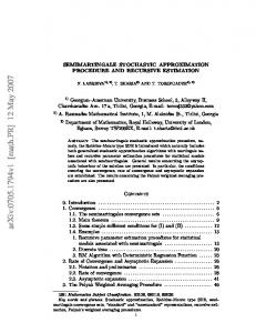
Stochastic Approximation approach discussed in Section III was used to optimize 𝜖 as a proof of concept. Hence, 𝜉, 𝛾, and 𝛽 were kept static at baseline settings, seen in Table I, of 𝜉 = 0.005, 𝛾 = 2.5, and 𝛽 = 3.5. Then 𝜖 was optimizing with by consideration ±c, with 𝒉𝟎 = 0.025, consistent with [9]. Since prior work in finding optimal settings did not consider randomness issues, to account for this, Nrep = 10 replicates were considered. Optimization was considered with respect to a maximum possible RAP value of 100 %C for all explored SNR operating points. To avoid training on testing data, optimization was performed with respect to the TNG set performance. The stochastic approximation approach was allowed to run continuously, using the absolute value between the RAP values seen in the last two iterations was 0.001. This resulted in Niter = 143 iterations being run. By evaluating the parameter settings, we see the learning rate’s progression plateauing at approximately 50 iterations. From here, the algorithm is seen slowly refining the learning rate’s value. When we consider the classification results associated with the final iteration, we see Fig. 6 which presents classification performance, all for the TST set, of %C versus SNR for: 1) GRLVQI - SD, which is GRLVQI after Stochastic Optimization, 2) GRLVQI – baseline, Baseline GRLVQI using the nominal settings of [37], and 3) MDA. Notably, we see that GRLVQI outperforms MDA. When GRLVQI’s learning rate is optimized via stochastic approximation, classification performance is seen to improve at low SNR (5 – 15 dB), degrade slightly at mid-range SNR (15 – 17 dB), and offer consistent performance to the baseline GRLVQI algorithm at high SNR (17 – 25 dB). Table 1 condenses the results, with gain and RAP values computed relative to MDA. Here we see that GRLVQI outperforms MDA and the baseline GRLVQI significantly. GRLVQI with a learning rate optimized via stochastic approximation is seen to offer only comparable classification and verification performance to the baseline GRLVQI in this table. However, it should be noted that a +6.45 dB gain at 60 %C was realized due to this optimization. Thus stochastic approximation is a viable method for finding operating points for GRLVQI.

Table 1. Algorithm Optimization Results PERFORMANCE RESULTS FACTORS LEVELS METHOD

MAX. OBJECTIVE A

Stochastic Approximation Optimization on 𝜖 Best Full Factorial [7] None [7]

B

C

D

VERIFICATION

CLASSIFICATION

E

GSNR (DB) AT %C = 90%

AT SNR = 20DB

RAP

TNG

TST

TNG

TST

TVR

AUCM

RAPTNG

0.0376

0.005

2.5

0.35

7

+3.51

+3.11

1.14

1.13

33%

0.950

Spreadsheet Search Constrained Nonlinear Optimization BASELINE GRLVQI MDA

0.25

0.05

2.0

0.35

7

+5.30

+5.77

1.22

1.18

66%

0.979

0.1501

0.05

4.5

0.15

7

+5.23

+5.26

1.20

1.19

66%

0.967

0.025 N/A

0.005 N/A

2.5 N/A

0.35 N/A

10 N/A

+3.72 +1.68

+3.32 0.00

1.14 1.23

1.13 1.0

33% 100%

0.936 0.971

V. CONCLUSIONS

Learning Rate

0.04

90 80 70 60 50

GRLVQI - SD, T st GRLVQI - baseline, T st

40

MDA, T st

30

0

5

10 15 SNR (dB)

20

25

Fig. 6. Representative classification performance for the TST set for the baseline GRLVQI algorithm, GRLVQI after Stochastic Optimization, and MDA.

0.035

VII. BIBLIOGRAPHY

0.03

0.025

100

Ave Pct Correct (%C)

Herein, the authors presented a proof-of-concept in applying stochastic approximation to find optimal algorithm settings for the learning rate of the GRLVQI neural network algorithm. One advantage of this approach over experimental design approaches is that parameter settings are free change without enforcing bounds, e.g. [7]. Furthermore, this stochastic approximation approach asymptotically converges to a (locally) optimal hyperparameter setting with probability one. While an improvement in low-SNR classification was seen, with +6.45 dB gain at 60% classification accuracy for TST data, overall performance was consistent with prior work. However, the proof-of-concept approach considered optimizing only one parameter with the other parameters held static. Further work, e.g. [38], is planned and will be considered by extending this process to all continuous GRLVQI parameters with an aim for improving overall performance.

0

50 100 Iteration Number

150

Fig. 5. Learning rate settings through 143 iterations

VI. ACKNOWLEDGEMENTS The authors would like to thank the Air Force Institute of Technology’s STAT in T& E Center of Excellence (COE) for its funding and support in this research effort. U.S. Government work is not protected by U.S. copyright. The views and conclusions contained herein are those of the authors and should not be interpreted as necessarily representing the official policies, either expressed or implied, of the Air Force Research Laboratory, the Air Force Institute of Technology or the U.S. Government.

[1] M. Knight, "How safe is Z-Wave?[Wireless standards]," Computing and Control Engineering, vol. 17, no. 6, pp. 18-23, 2006. [2] C. Gomez and J. Paradells, "Wireless home automation networks: A survey of architectures and technologies," IEEE Communications Magazine, pp. 92-101, June 2010. [3] S. Prabhakar, S. Pankanti and A. K. Jain, “Biometric recognition: Security and privacy concerns,” IEEE Security Privacy, pp. 33-42, March/April 2003. [4] W. E. Cobb, E. D. Laspe, R. O. Baldwin, M. A. Temple and Y. C. Kim, "Intrinsic physical-layer authentication of integrated circuits," IEEE Transactions on Information Forensics and Security, vol. 7, no. 1, pp. 14-24, 2012. [5] T. J. Bihl, M. A. Temple, K. W. Bauer and B. W. Ramsey, "Dimensional Reduction Analysis for Physical Layer Device Fingerprints with Application to ZigBee and Z-Wave Devices," Military Communications Conference (MILCOM), pp. 360-365, 2015. [6] T. J. Bihl, K. W. Bauer and M. A. Temple, "Feature Selection for RF Fingerprinting With Multiple Discriminant Analysis and Using ZigBee Device Emissions," IEEE Transactions on Information Forensics and Security, vol. 11, no. 8, pp. 18621874, 2016. [7] T. Bihl, M. Temple and K. Bauer, "An Optimization Framework for Generalized Relevance Learning Vector Quantization with Application to Z-Wave Device Fingerprinting," Hawaii International Conference on System Sciences (HICSS), pp. 2379-2387, 2017. [8] M. J. Mendenhall, A Neural Relevance Model for Feature Extraction from Hyperspectral Images, and its Application in the Wavelet Domain, PhD Dissertation: Rice University, 2006. [9] P. K. Harmer, D. R. Reising and M. A. Temple, "Classifier selection for physical layer security augmentation in Cognitive

[10]

[11] [12]

[13]

[14]

[15]

[16]

[17]

[18]

[19]

[20]

[21]

[22]

[23]

[24]

Radio networks," IEEE International Conference on Communications (ICC), pp. 2846-2851, 2013. B. Hammer and T. Villmann, "Generalized relevance learning vector quantization," Neural Networks, vol. 15, no. 8-9, pp. 1059-1068, 2002. T. Kohonen, "Learning vector quantization," Self-Organizing Maps, pp. 175-189, 1995. A. S. Sato and K. Yamada, "Generalized learning vector quantization," in Advances in neural information processing systems, Cambridge, MA, MIT Press, 1995, pp. 423-429. A. I. Gonzalez, M. Grana and A. D'Anjou, "An analysis of the GLVQ algorithm," IEEE Transactions on Neural Networks, vol. 6, no. 4, pp. 1012-1016, 1995. T. Bojer, B. Hammer, D. Schunk and K. Tluk von Toschanowitz, "Relevance determination in learning vector quantization," Proceedings of European Symposium on Artificial Neural Networks (ESANN), pp. 271-276, 2001. M. J. Mendenhall and E. Merenyi, "Relevance-Based Feature Extraction for Hyperspectral Imagery," IEEE Transactions on Neural Networks, vol. 19, no. 4, pp. 658-672, 2008. M.-T. Vakil-Baghmisheh and N. Pavesic, "Premature clustering phenomenon and new training algorithms for LVQ," Pattern Recognition, vol. 36, pp. 1901-1912, 2003. W. Zhang and A. T. Goh, "Reliability assessment on ultimate and serviceability limit states and determination of critical factor of safety for underground rock caverns," Tunnelling and Underground Space Technology, vol. 32, pp. 221-230, 2012. J. Bellucci, T. Smetek and K. Bauer, "Improved hyperspectral image processing algorithm testing using synthetic imagery and factorial designed experiments," IEEE Transactions on Geoscience and Remote Sensing, vol. 48, no. 3, pp. 1211-1223, 2010. C.-C. Chiu, D. F. Cook, J. P. Pignatiello and A. D. Whittaker, "Design of a radial basis function neural network with a radiusmodification algorithm using response surface methodology," Journal of Intelligent Manufacturing, vol. 8, no. 2, pp. 117-124, 1997. A. Glyk, D. Solle, T. Scheper and S. Beutel, "Optimization of PEG–salt aqueous two-phase systems by design of experiments," Chemometrics and Intelligent Laboratory Systems, vol. 149, pp. 12-21, 2015. L. Wu, K. Yick, S. Ng and J. Yip, "Shape characterization for optimisation of bra cup moulding," Journal of Fiber Bioengineering and Informatics, vol. 4, no. 3, pp. 235-243, 2011. X. Yang, J. Li, Z. Fang and C. Wang, "The Optimum Design of Gear Transmission Based on MATLAB," International Conference on Measuring Technology and Mechatronics Automation (ICMTMA), vol. 3, pp. 925-928, 2010. J. Kiefer and J. Wolfowitz, "Stochastic estimation of the maximum of a regression function," The Annals of Mathematical Statistics, vol. 23, no. 3, pp. 462-466, 1952. ITU, ITU-T G.9959: Short range narrow-band digital radio communication transceiver - PHY and MAC layer specifications, Geneva, Switzerland: International Telecommunication Union, 2012.

[25] C. Badenhop, B. Ramsey, B. Mullins and L. Mailloux, "Extraction and analysis of non-volatile memory of the ZW0301 module, a Z-Wave transceiver," Digital Investigation, vol. 17, pp. 14-27, 2016. [26] J. D. Fuller and B. W. Ramsey, "Rogue Z-Wave controllers: A persistent attack channel," Local Computer Networks Conference Workshops (LCN Workshops), pp. 734-741, 2015. [27] C. Badenhop, J. Fuller, J. Hall, B. Ramsey and M. Rice, "Evaluating ITU-T G. 9959 Based Wireless Systems used in Critical Infrastructure Assets," International Conference on Critical Infrastructure Protection, pp. 209-227, 2015. [28] M. Galeev, "Catching the Z-Wave," Electronic Engineering Times India, pp. 1-5, Oct. 2006. [29] W. E. Cobb, E. W. Garcia, M. A. Temple, R. O. Baldwin and Y. C. Kim, "Physical layer identification of embedded devices using RF-DNA fingerprinting," Military Communications Conference (MILCOM), pp. 2168-2173, 2010. [30] C. K. Dubendorfer, B. W. Ramsey and M. A. Temple, “ZigBee device verification for securing industrial control and building automation systems,” Int. Conf. on Critical Infrastructure Protection (IFIP13), vol. 417, pp. 47-62, 2013. [31] C. K. Dubendorfer, B. W. Ramsey and M. A. Temple, "An RFDNA verification process for ZigBee networks," Military Communications Conference (MILCOM), pp. 1-6, 2012. [32] T. Kohonen, J. Kangas, J. Laaksonen and K. Torkkola, "LVQ_PAK: A program package for the correct application of Learning Vector Quantization algorithms," Proceedings of the International Joint Conference on Neural Networks, pp. 725730, 1992. [33] M. Kaden, M. Lange, D. Nebel, M. Riedel, T. Geweniger and T. Villmann, "Aspects in classification learning-Review of recent developments in Learning Vector Quantization," Foundations of Computing and Decision Sciences, vol. 39, no. 2, pp. 79-105, 2014. [34] D. DeSieno, "Adding a conscience to competitive learning," Proceedings of the IEEE International Conference on Neural Networks, pp. 117-124, 1988. [35] M. Strickert, U. Seiffert, N. Sreenivasulu, W. Weschke, T. Villmann and B. Hammer, "Generalized relevance LVQ (GRLVQ) with correlation measures for gene expression analysis," Neurocomputing, vol. 69, no. 7-9, pp. 651-659, 2006. [36] C. Dubendorfer, B. Ramsey and M. Temple, "ZigBee device verification for securing industrial control and building automation systems," International Conference on Critical Infrastructure Protection, pp. 47-62. [37] D. R. Reising, M. A. Temple and J. A. Jackson, "Authorized and rogue device discrimination using dimensionally reduced rf-dna fingerprints," IEEE Transactions on Information Forensics and Security, vol. 10, no. 6, pp. 1180-1192, 2015. [38] T. J. Bihl and D. W. Steeneck, "Multivariate Stochastic Approximation to Tune Neural Network Hyperparameters for Criticial Infrastructure Communication Device Identification," Hawaii International Conference on System Sciences, 2018.