StochKit-FF: Efficient Systems Biology on Multicore Architectures

` di Pisa Universita

arXiv:1007.1768v1 [cs.CE] 11 Jul 2010

Dipartimento di Informatica

Technical Report: TR-10-12

StochKit-FF: Efficient Systems Biology on Multicore Architectures Marco Aldinucci Andrea Bracciali Pietro Li`o Anil Sorathiya Massimo Torquati

July 1, 2010 ADDRESS: Largo B. Pontecorvo 3, 56127 Pisa, Italy.

TEL: +39 050 2212700

FAX: +39 050 2212726

StochKit-FF: Efficient Systems Biology on Multicore Architectures Marco Aldinucci

∗

Andrea Bracciali†

Anil Sorathiya§

Pietro Li`o‡

Massimo Torquati¶

July 1, 2010

Abstract The stochastic modelling of biological systems is an informative, and in some cases, very adequate technique, which may however result in being more expensive than other modelling approaches, such as differential equations. We present StochKit-FF, a parallel version of StochKit, a reference toolkit for stochastic simulations. StochKit-FF is based on the FastFlow programming toolkit for multicores and exploits the novel concept of selective memory. We experiment StochKit-FF on a model of HIV infection dynamics, with the aim of extracting information from efficiently run experiments, here in terms of average and variance and, on a longer term, of more structured data. Keywords: stochastic models, parallel computing, multicore, systems biology.

1

Introduction

The immune system is an example of a complex system formed out of its intercellular and intracellular components, which organise in space and time the immune response to pathogens through a system of regulatory nested feedbacks, both positive and negative. The modelling of part of the immune response to HIV infection is a paradigmatic scenario illustrating the challenges that computerbased modelling and analysis present for this class of problems. The immune system can be modelled by deterministic equations or by stochastic modelling approaches. Differential equations (ODEs) are effective in characterizing the system dynamics when the molecular copy number of each species is sufficiently ∗ Computer

Science Department, University of Torino, Italy - CNR, Italy ‡ Computer Laboratory, Cambridge University, UK § Computer Laboratory, Cambridge University, UK ¶ Computer Science Department, University of Pisa, Italy † ISTI

1

large. Whenever the number of molecules considered is small, then a stochastic model is much more accurate on a mesoscale. The numerical solvability of stochastic models is limited to pretty small dimensions (e.g. number of species) due to their exponential complexity. The behaviour of larger systems can be described by stochastic simulations, such as those based on the Gillespie’s algorithm, a Monte Carlo method simulating the system dynamics step by step. These methods are more accurate than the deterministic ones for describing many phenomena, however they can be highly demanding in terms of computational power, for instance when many simulations are considered for precisely characterising the overall behaviour of the system. Stochastic methods represent the most challenging methodological areas of system biology and will play a growing role in modelling, amongst the others, immune system responses to pathogens. We here illustrate the use of parallelism for supporting efficient and informative stochastic analysis of one such model. Multiple simulations exhibit a natural independence that would allow them to be treated in an embarrassingly parallel fashion. However, this is not possible whenever the results need to be concurrently combined or compared. In many cases, recombination is done in a post-processing phase as a sequential process whose cost in time and space depends on the number and the size of the simulation results and might be comparable to the cost of the simulation phase. A second important aspect regards execution performance: independent simulations exhibit good parallel scalability only if executed onto truly independent platforms (such as multicomputers, cluster or grid), but they might exhibit serious performance degradation if run on multicore due to the concurrent usage of underlying resources. This effect is particularly significative for I/O-bound applications since typically I/O and memory buses are shared among cores. In this paper we introduce StochKit-FF, a parallel version of the popular StochKit framework [12], aiming at supporting the execution of multiple simulations and at combining their results on cache-coherent, shared memory multicores. This kind of architectures has been recently embraced by the whole computer industry and they equip a large range of computing platforms. StochKit-FF has been designed and developed as a low-effort, efficient porting of the StochKit main simulation loop by means of the FastFlow C/C++ programming framework, which supports efficient applications on multicore. FastFlow makes it possible to run multiple parallel stochastic simulations and to combine their results. This relies on selective memory, a novel data structure we designed to perform the online alignment and reduction of multiple streams of simulation results: different data streams are aligned according to simulation time and combined together according to a user-defined function, e.g. the average or others. By discussing the HIV case-study, we intend to show that this framework represents an efficient way for running multiple simulations and a promising direction for the development of effective modelling techniques, currently centered on distilling averaged values, but also more structured and informative data types on a longer term project. Next, we summarise aspects of the immune response to HIV, recapitulate how 2

stochastic simulations work and introduce our model. Then we overview FastFlow and present StochKit. A section on experimental results follows before some concluding remarks.

2

A stochastic model of the immune response to HIV

Ordinary differential equations (ODEs) based models have long been used for immune system and viral infection modeling [11, 15, 14]; they focus on the average behavior of large populations of identical objects; large complex system of nonlinear equations need often be solved numerically. When considering a small number of molecules, which is highly probable if we consider immune cell interactions in a small volume or if the reactions occur far from thermodynamic equilibrium, or when considering randomness and irregularities found at all levels of life, such as the random motion of cellular components, then a stochastic model is much more accurate on a mesoscale. For instance, the master equation is a differential-difference equation for the time-dependent probability density of the number of molecules of each species. Stochastic methods are those based on the Gillespie’s algorithm, a Monte Carlo method simulating the reactions step by step [8]. Such stochastic methods are more effective than the deterministic ones to describe the above mentioned irregularities and also crucial chemical reactions. We adopt an agent-based approach: simulation considers the actions of a large number of simple entities, or agents (viruses and cells), in order to observe emerging properties from their interaction, which is based on local rules [6]. Briefly, each agent consists of state variables and a set of rules that govern its behavior. Agents can interact either directly with each other or indirectly through the environment. Agent behaviour consists of actions, e.g. cellular interactions, that cause a state transition of the modelled system, e.g. a variation in the amount of agents. Actions are stochastic in the sense that their occurrence in time has an associated probability. Associated probability distributions are generally memoryless, typically negative exponential distributions with the rate as parameter, and hence the overall system behaviour can be interpreted as a Continuous Time Markov Chain (CTMC). Systemic emergent properties can be sensitive to the local presence of minimal (integer) quantities of agents/molecules/cells [18]. The combined behavior of these agents is observed in a discrete-time or event-driven stochastic simulation, from given initial conditions. Given the current state of the system, a single transition amongst the possible ones is selected, and the state updated accordingly. The Gillespie’s algorithm [8] determines the next transition and the time at which it occurs, exactly according to the given probability distributions. Each sodetermined possible evolution of the system is called a trajectory. Long time and large computing resources may be required in order to correctly evaluate parameters and determine fluctuations and averages of the system behaviour

3

λ

→ U0 + U U0 − δuf

U +F − −− →F δut

U −−→ T δ

−uz − → Z4 U − δuz

−− → Z5 U −

δtf

T + F −−→ F βR5

T + V5 −−−→ I5 βX4

T + V4 −−−→ I4 γ

−→ I5 Z5 + V5 −−R5 γX4

Z4 + V4 −−−→ I4

σ

2 I5 −−→ I5 + Z 5 σ2

I4 −−→ I4 + Z4 σ1

I5 + Z5 −−→ U + I5 + Z5 σ

1 I4 + Z4 −−→ U + I4 + Z 4 δiz

I5 + Z5 −−→ Z5 δ

δ

t − → 0 T −

iz I4 + Z4 −− → Z4

δ

µ

z − → 0 Z5 −

→ V5 × 200 I5 −

π

z − → 0 Z4 −

π

δv

V5 − → V4

→ V4 × 200 I4 − σ

3 V4 −−→ F + V4

δ

− →0 V5 − δ

v − → 0 V4 −

δi

I5 −→ 0 δ

i I4 −→ 0

Table 1: Reaction-centric view of the HIV model. when simulating trajectories.

2.1

HIV and the immune response in formulae

The model we are drafting in this section follows those in [11, 16] and is sketched as simply but meaningfully as possible, given its purposes here. During the HIV infection multiple strains of the virus arise, we consider two phenotype classes, V 5 and V 4. They allow virus entry in cells through two membrane receptors, CCR5 and CXCR4, respectively. The mutation from V 5, initially prevailing, to the more aggressive V 4 has been correlated with a faster progression of the disease to the AIDS phase. The immune response is based on the action of several cells, some of which strain specific (T, Z5 and Z4), which can also be infected by the viruses. We also consider the Tumor Necrosis Factor F , which induces bystander death of several cells. Infection is characterised by the progressive loss of T cells, infected together with Z5 and Z4 by the virus in order to proliferate. The set of possible reactions is reported in Table 1, according to a reactioncentric view, while the behaviour of a specific agent is determined by the union of the reactions to which it participates. Reactions are labeled with their stochastic rates and are commented below. Mature (uninfected) T cells have precursors, the immature Naive T cells (U ), produced at a constant rate λ (200C/µlt−1 , with C/µl cells per micro-liter and t−1 the inverse of time). U cells are transformed into mature T cells with rate δut (0.129t−1 ), and also into Z4 and Z5 cells with rate δuz (0.005t−1 ), and are cleared out by the interaction with F (Tumor Necrosis Factor, a cytokine) with rate δuf (10−5 µl/Ct−1 ). T cells are cleared with rate δt (0.01t−1 ). The increase of F causes the death of the T cells at rate δtf (10−5 µl/Ct−1 ). Viral strains V 5 and V 4 interacting with T cells produce infected cells I5 and I4 at rate βR5 and βX4 respectively. Similarly, V 5 and V 4 interacting with Z5 and Z4 cells produce infected cells at rate γR5 and γX4 , respectively. The strains Z5 and Z4 are cleared at rate δz (0.01t−1 ). Z cells proliferate due to infection in the system with the proliferation rate σ2 (0.001µl/Ct−1 ). Moreover, the production of U cells increases due to the presence of Z and infected cells at rate σ1 (0.0001µl/Ct−1 ). This is a simplifying working hypothesis: the effects of the presence of Z and I, i.e. the increase of U , are modelled rather than the actual mechanisms that lead to

4

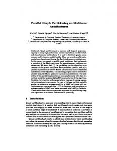
Figure 1: HIV Model: a single trajectory. 1. (left) The immune cell dynamics is shown over a time span of 4000 days. It is evident both the “noisy” nature of cell time courses and the V 5 − V 4 mutation at about day 1000. Note how the most aggressive strain V 4 defeats T cells (An amount of T cells less than about 200 is considered the threshold for AIDS). 2. (right) Also the virus V 5 + V 4 is reported on a log-scale, which highlights the effects of the mutation on the virus (note the high peak perturbation) and coincidently on the immune system, and also the dynamics for small amounts of cells. the generation of new U s (via the dendritic cells signalling to naive T cells for optimal activation [9]). The infected cells are killed by Z cells with rate δiz (0.06 µl/C t−1 ). Mutation of V 5 strains into V 4 strains happens at rate µ (2.5 × 10−3 ). The bursting of infected cells produces about 200 viruses at rate π (200µl/Ct−1 ). The accumulation of F is proportional to the total amount of V 4 viruses, and happens at a rate σ3 (0.0001t−1 ). The infected cells are cleared at rate δi (0.33t−1 ). Viruses are cleared at rate δv (2t−1 ). The parameters used have been referred from literature, e.g. [11, 15, 14, 17, 13] and sometimes tuned against known aspects of the macroscopic behaviour of the system. The initial conditions for the simulations of our system are: U 0 = 1, U = 200, T = 1000, Z4 = 250, Z5 = 250, I4 = 0, I5 = 0, V 4 = 0, V 5 = 100, F = 0. The infectivity of V 5 and V 4 depends on the concentration of TNF in the system. Initially, in the absence of F , the infectivity rate is constant, β = 4 × 10−5 µl/C t−1 for both V 5 and V 4. When V 4 appears, βR5 = β −K ∗F decreases and βX4 = β +K ∗F increases because of the amount of F (K = 10−7 (µl/C)2 t−1 and 0 ≤ βR5 ≤ β). Analogously: γR5/X4 = γ ∓K ∗F (γ = 2 × 10−5 µl/C t−1 ). It is worth pointing out, as a modelling methodology, that we embedded a notion of time in the model by means of a stochastic event expected to occur at about a given time instant and used to trigger the V 5 to V 4 mutation at a certain stage of the disease progression. Figure 1 reports a trajectory of our model. Next section will introduce the framework that allowed it to be computed.

5

3

Parallel Stochastic Simulations

In Monte Carlo simulations, each individual trajectory represents just one possible way in which the system might have reacted over the entire simulation time-span. Many trajectories might be needed to get a representative picture of how the system behaves on the whole. Processing and combining many trajectories may lead to very high compulsory cache miss-rate and thus become a memory-bound (and I/O-bound) problem. This in turn may require a huge amount of storage space (linear in the number of simulations and the observation size of the average trajectory) and an expensive post-processing phase, since data should be retrieved from permanent storage and processed. Eventually, the computational problem hardly benefits from the latest commodity multi-core architectures. These architectures are able to exhibit an almost perfect speedup with independent CPU-bound computations, but hardly replicate such a performance for memory-bound and I/O-bound computations, since the memory is still the real bottleneck of this kind of architectures. Tackling these issues at the low-level is often unfeasible because of the complexity of the code and of the need to keep the application code distinct from platform-specific performance tricks. Typically, low-level approaches only provide the programmers with primitives for flow-of-control management, synchronisation and data sharing. In this regard, the shared memory paradigm, which is natively supported by multicores, is often and incorrectly considered simpler with respect to message passing paradigm. While writing a first working prototype is certainly faster, tuning it for performance is often a nightmare due to the non-trivial effects induced by memory fences (used to implement mutex) on data replicated in core’s caches. Designing suitable high-level abstractions for parallel programming is a long standing problem [5]. Recently, high-level parallel programming methodologies are receiving a renewed interest, especially in the form of pattern-based programming [7, 10, 4]. FastFlow belongs to this class of programming environments.

3.1

The FastFlow Parallel Programming Environment

FastFlow is a parallel programming framework aiming at simplifying the development of efficient applications for multicore platforms, being these applications either brand new or ports of existing legacy codes. The key vision underneath FastFlow is that effortless development and efficiency can both be achieved by raising the level of abstraction in application design, thus providing designers with a suitable set of parallel programming patterns that can be compiled onto efficient networks of parallel activities on the target platforms. To fill the abstraction gap, as shown in Figure 2, FastFlow is conceptually designed as a stack of layers that progressively abstract the shared memory parallelism at the level of cores up to the definition of useful programming constructs and patterns. At the lowest tier of the FastFlow system we have the architectures that it targets: cache-coherent multiprocessors, and in particular commodity homoge6

Efficient applications for multicore and manycore Smith-Waterman, N-queens, QT, C4.5, FP-Growth, ...

Applications

Autonomic Behav.Skeletons

Problem Solving Environment

FastFlow

StochKit instances

Simulation StochKit-FF

Streaming networks patterns Skeletons: Pipeline, farm, D&C, ...

High-level programming Low-level programming

Accelerator self-offloading

Simulation instances dispatching

Arbitrary streaming networks (building blocks) Lock-free SPSC, SPMC, MPSC, MPMC queues

Run-time support

Simple streaming networks (building blocks) Lock-free SPSC queues and general threading model

Hardware

Multi-core and many-core cc-UMA or cc-NUMA featuring sequential or weak consistency

Result gathering via Selective Memory

W1 input stream

E

C Wn

Farm

E

output stream

C

SPMC

MPSC P

C

lock-free SPSC queue Producer Consumer

Figure 2: FastFlow layered architecture with pattern examples.

nous multicore (e.g. Intel core, AMD K10, etc.). The second tier provides mechanisms to define simple streaming networks whose run-time support is implemented through correct and efficient lock-free Single-Producer-Single-Consumer (SPSC) queues. This kind of queues do not require (under mild requirements [1]) any lock or memory barrier, and thus they constitute a solid ground for a low-latency synchronization mechanism for multicore. These synchronizations, which are asynchronous and non-blocking, do not induce any additional cache invalidation as it happens in mutual exclusion primitives, and thus do not add a significant overhead. The third tier generalises one-to-one to one-to-many (SPMC), many-to-one (MPSC) and many-to-many (MPMC) synchronizations and data flows, which are implemented using only SPSC queues and arbiter threads. This abstraction is designed in such a way that arbitrary networks of activities can be expressed while maintaining the high efficiency of synchronisations. The next layer up, i.e., high-level programming, provides a programming framework based on parallelism exploitation patterns (a.k.a. skeletons [5]). They are usually categorised in three main classes: Task, Data, and Stream Parallelism. FastFlow specifically focuses on Stream Parallelism, and in particular provides: farm, farm-with-feedback (i.e. Divide&Conquer), pipeline, and their arbitrary nesting and composition. These high-level skeletons are actually factories for parametric patterns of concurrent activities, which can be instantiated with sequential code or other skeletons, then cross-optimised and compiled together with lower FastFlow tiers. The skeleton disciplines concurrency exploitation within the generated parallel code: the programmer is not required to explicitly interweave the business code with concurrency related primitives. The set of skeletons provided by FastFlow could be further extended by building new C++ templates or even further abstracted to derive problem specific skeletons. We refer to [3] for any further details. FastFlow is open source available at http://sourceforge.net/projects/mc-fastflow/ under LGPL3.

7

3.2

Parallel StochKit: StochKit-FF

StochKit [12] is an efficient, extensible stochastic simulation framework developed in the C++ language. It aims at making stochastic simulation accessible to practicing biologists and chemists, while remaining open to extension via new stochastic and multi-scale algorithms. It implements the popular Gillespie algorithm, explicit and implicit tau-leaping, and trapezoidal tau-leaping methods. StochKit-FF extends StochKit v1 with two main features: The support for the parallel run of multiple simulations on multicores, and the support for the online (parallel) reduction of simulation results, which can be performed according to one or more user-defined associative and commutative functions. StochKit v1 is coded as a sequential C++ application exhibiting several nonreentrant functions, including the random number generation.1 Consequently, StochKit-FF represents a significative test bed for the FastFlow ability to support parallelisation of existing complex codes. The parallelisation is supported by means of high-level parallel patterns, which could also be exploited as parametric code factories to parallelise existing, possibly complex C/C++ codes [1]. In particular, StochKit-FF exploits the FastFlow farm pattern, which implement the functional replication paradigm: a stream of independent data items are dispatched by an Emitter thread to a set of independent Worker threads. Each worker produces a stream of results that is gathered by a Collector thread into a single output stream. The farm paradigm is sketched in Figure 2. In StochKit, a simulation is invoked by way of the StochRxn(), which realises the main simulation loop. The propensity function and initial conditions are among its parameters. StochKit-FF provides the programmer with StochRxn ff() function, which has a similar list of parameters, but invokes a parametric simulation modelling either a number of copies of the same simulation or a set of parameter-sweeped simulations. StochRxn ff() embodies a farm: the emitter unrolls the parametric simulation into a stream of standard simulations (represented as C++ objects) that are dispatched to workers. Each worker receives a set of simulations, which are sequentially run by way of the StochRxn(), which is basically unchanged2 with respect to the original StochKit. Each simulation produces a stream of results, which are locally reduced within each worker into a single stream [5]. The collector gathers all worker streams and reduces them again into a single output stream. In the case it is required, the worker can directly write the full simulation results of all simulations into different files. Overall, the parallel reduction happens in a systolic (tree) fashion via the so-called selective memory data structure. 1 At the time of writing, a new beta multithreaded version of StochKit has been made available. However, also this new version does not offer the possibility to combine trajectories from different simulations, which are written into different files. 2 It is made thread-safe by substituting the sprng random generator with boost.

8

25

Sim1 Sim2 Sim3 Avg-Y Avg-XY

20 Amount (units)

20 Amount (units)

25

Sim1 Sim2 Sim3 Avg-Y

15 10 5

15 10 5

0 0

1

2

3

4

5

6 7 Time

8

0

9 10 11 12 13

0

1

2

3

4

5

6 7 Time

8

9 10 11 12 13

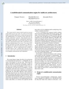
Figure 3: Selective Memory with average. 1. (left) Curve Avg-Y is derived via oversampling and time-aligned reduction (average along Y axis) of k independent simulations (arrows highlight oversampling). 2. (right) Avg-XY is derived by the reduction (average along X axis) of k successive points of Avg-Y (grey boxes highlight averaging zone). 3.2.1

Selective Memory

Together with StochKit-FF, we introduce the selective memory concept, i.e. a data structure supporting the on-line reduction of time-aligned trajectory data by way of one or more user-defined associative and commutative functions. Selective memory distinguishes from standard parallel reduce operation [5, 2] because it works on (possibly unbound) streams, and aligns simulation points (i.e. stream items) according to simulation time before reducing them: since each simulation proceed at a variable time step, simulation points coming from different simulations cannot simply be reduced as soon as they are produced. Selective memory behaves as an array of buffers that abstractly realise a sliding window that follows the wavefront of generated simulation points along simulation time. It keeps the bare minium amount of simulation points from different simulation to produce a slice of aligned simulation points, which are popped from selective memory as soon as they are reduced. The behaviour of selective memory is exemplified in Figure 3 using average as combining function. Simulation points from different simulations are first averaged at aligned simulation time points: such computed average results oversampled with respect to single simulations (Figure 3 left). This oversampling is possibly reduced by applying the same technique along time axis (Figure 3 right). Overall, selective memory produces a combined simulation that has been adaptively sampled: time intervals exhibiting a higher variability across different simulations exhibit an higher sampling rate. Selective memory effectively mitigates the memory pressure of result logging when many simulations are run on a multicore, because it substantially reduces the output size, and thus capacity misses and the memory bus pressure. The StochKit-FF implementation of the HIV model. StochKit-FF main9

1K

T(A) Z4(A) Z5(A) Z(A) Amount (units)

Amount (units)

800 600 400 200

8K 6K 4K 2K

0 0

25K

0 500 1000 1500 2000 2500 3000 3500 4000 Time (days)

20

10K 5K

40 60 Time (days)

80

100

T(A) Z4(A) Z5(A) Z(A) V(A)

120K Amount (units)

15K

0

140K

T(A) Z4(A) Z5(A) Z(A) V(A)

20K Amount (units)

T(A) Z4(A) Z5(A) Z(A) V(A)

10K

100K 80K 60K 40K

0 20K 0 0

500 1000 1500 2000 2500 3000 3500 4000 Time (days)

0

500 1000 1500 2000 2500 3000 3500 4000 Time (days)

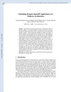
Figure 4: HIV Model: average and variance for multiple trajectories (16x). Left to right: 1. A focus on the immune response. 2-4 Sensitivity analysis for δt = 5.0, 3.0 and 0.5. tains the same interface of StochKit. A model is specified by providing C++ files containing the needed information in suitable data structure. In our case: i) a list of constant definitions for all the parameters used; ii) an integer state vector with an entry for each species in the model, initialised with the initial conditions for the simulation; iii) an integer stoichiometric matrix with an entry i, j for the amount of the i-th species involved in the j-th reaction, e.g. −1 for π a consumed species or 200 for the viruses released by I4 − → V4 × 200 (Table 1); and iv) the propensity vector associating to each reaction its propensity, then employed by the Gillespie algorithm in the selection of the next reaction. In our case, reactions follow the law of mass action and depend on the amount of reactants and the associated rates, intuitively the more the reactants (and the rate) the highest the probability of being selected, e.g. I4 × π for the previous reaction. Finally, the desired duration of the simulation interval has to be specified.

10

16

ideal 32 runs 64 runs 128 runs

16 14

Scalability (against StochKit-FF)

Speedup (against StochKit)

18

12 10 8 6 4 2 0 0

2

4

6 8 10 N. of workers

12

14

12 10 8 6 4 2 0

16

ideal 32 runs 64 runs 128 runs

14

0

2

4

6 8 10 N. of workers

12

14

16

Figure 5: 1. (left) Speedup of StochKit-FF against StochKit. 2. (right) Scalability of StochKit-FF(n) against StochKit-FF(1), where n is the number of worker threads.

4

Experiments and Discussion

We report on some experiments performed on the ness.epcc.ed.ac.uk platform (Sun X4600 SMP - 8 x Dual-Core AMD Opteron 1218, 32 Gb memory) hosted at EPCC, University of Edinburgh. Figure 4 (top-left) is a focus on the immune response averaged over 16 simulations. The averaged amounts of Z4, Z5, their sum Z, and T are reported together with a representation of their variance (obtained by rough summation). The variance of Z4 and Z5 is large till 2500 days, showing tight coupling i.e. interdependence. Then, the variance of T decreases continuously, while the one of Z5 decreases together with the (averaged) amount of Z5, as it is not much involved in dynamics after the mutation to V 4, while the number of the budding viruses still have high probability of infecting and killing cells. The other three pictures in Figure 4 describe a sensitivity analysis for δt , the parameter regulating the lifespan of the virus and originally set to 1.5. By a large analysis of the model, δt has resulted in being very influential on the emerging behaviour of the system as it strongly impacts on the diffusion of the infection. In 2 the virus is immediately cleared out (the picture is relative to the interval [1,100]), T rapidly increases, and the system is very stable, with a low variance. In 3 the immune response still prevails, but the system appears much perturbed. In 4, well below the standard value of δt , the virus clearly prevails. Initially variance is high, over large numbers for the viral load, then it tends to stabilise towards a steady state. The performances of StochKit-FF have been evaluated on multiple runs of the HIV case-study. A single run of the simulation with StochKit averagely produces ∼ 150M simulation points for 4000 days of simulated time, which will turn into about 6 GBytes of generated data; multiple runs of the same simulation will need a linearly greater time and space. These simulations can be naively parallelised on a multicore platform by running several independent instances, which however, will compete for memory and disk accesses, thus lead 11

to suboptimal performances in the case of high output pressure. Observe, as an example, that the HIV simulation with a 1:10 sampling (outputting 1 simulation point every 10) spends 64 seconds for the simulation and 133 seconds in the output phase on our testing platform. An additional linear time (at least) in the number and the size of outputs should be spent in the postprocessing phase for the recombination of results (6 MBytes per simulation per the number of runs). StochKit-FF mainly attacks these latter costs by online reducing the outputs of simulations, which are run in parallel. In Figure 5, average and variance are used as combining functions. As shown in Figure 5 (left), StochKit-FF exhibits a superlinear speedup with respect to StochKit in all tested cases (32, 64, 128 repetitions of the HIV simulation). This superlinear speedup is mainly due to the fact that StochKit-FF is about two times faster than StochKit even when running with just one thread. They are mainly due to FastFlow memory allocator that is faster than standard memory allocator on the tested platform, and some little code optimisation involving memory management that has been introduced during the port. As shown in Figure 5, StochKit-FF exhibits a good scalability also when compared with the sequential (one-thread) version of StochKit-FF.

5

Concluding remarks

We have introduced StochKit-FF, developed within FastFlow, which has supported the porting of a complex application with minimal modifications required. StochKit-FF allows multiple stochastic simulations of biological systems to be run efficiently and their results to be suitably combined according to the user needs. For the aims of recombinations, we have developed the concept of selective memory. For the development and for this presentation we have grounded StochKit-FF on a realistic model of HIV infection, as the stochastic analysis of this kind of systems is playing a growing role in systems biology. We have presented simulations and experiments for this model, highlighting aspects of the emerging behaviour of the system under different assumptions. As discussed, performances are convincing in terms of efficiency, close to optimality, and scalability. We are interested in further improving performances, in developing more informative recombining functions, which will allow more structured data to be extracted from multiple simulations, and in testing the framework on different domains.

Acknowledgments Marco Aldinucci and Andrea Bracciali have been partially supported by a grant of the HPC-Europa 2 Transnational Access programme. Marco Aldinucci has been partially supported by the BioBITs (“Developing White and Green Biotechnologies by Converging Platforms from Biology and Information Tech-

12

nology towards Metagenomic”).

References [1] Marco Aldinucci, Marco Danelutto, Peter Kilpatrick, Massimiliano Meneghin, and Massimo Torquati. Accelerating sequential programs using FastFlow and self-offloading. Technical Report TR-10-03, Universit`a di Pisa, Dipartimento di Informatica, Italy, February 2010. [2] Marco Aldinucci, Sergei Gorlatch, Christian Lengauer, and Susanna Pelagatti. Towards parallel programming by transformation: The FAN skeleton framework. Parallel Algorithms and Applications, 16(2–3):87–121, March 2001. [3] Marco Aldinucci, Massimiliano Meneghin, and Massimo Torquati. Efficient smith-waterman on multi-core with FastFlow. In Marco Danelutto, Tom Gross, and Julien Bourgeois, editors, Proc. of Intl. Euromicro PDP 2010: Parallel Distributed and network-based Processing, pages 195–199, Pisa, Italy, February 2010. IEEE. [4] Krste Asanovic, Rastislav Bodik, James Demmel, Tony Keaveny, Kurt Keutzer, John Kubiatowicz, Nelson Morgan, David Patterson, Koushik Sen, John Wawrzynek, David Wessel, and Katherine Yelick. A view of the parallel computing landscape. CACM, 52(10):56–67, 2009. [5] Bruno Bacci, Marco Danelutto, Salvatore Orlando, Susanna Pelagatti, and Marco Vanneschi. P3 L: a structured high level programming language and its structured support. Concurrency Practice and Experience, 7(3):225–255, May 1995. [6] L. Chao, M.P. Davenport, S. Forrest, and A.S. Perelson. A stochastic model of cytotoxic t cell responses. Journal Theoretical Biology, 228:227– 240, 2004. [7] Jeffrey Dean and Sanjay Ghemawat. MapReduce: Simplified data processing on large clusters. In Usenix OSDI ’04, pages 137–150, December 2004. [8] D.T. Gillespie. Exact stochastic simulation of Coupled Chemical Reactions. The Journal of Physical Chemistry, 81(25):2340–2361, 1977. [9] P. Guermonprez, J. Valladeau, L. Zitvogel, C. Thery, and S. Amigorena. Antigen presentation and T cell stimulation by dendritic cells. Annual Review of Immunology, 20:621–667, 2002. [10] Intel Corp. Intel Threading Building Blocks, July 2009. http://software. intel.com/en-us/intel-tbb/.

13

[11] A.S. Perelson, A.U. Neumann, M. Markowitz, J.M. Leonard, and D.D. Ho. HIV-1 dynamics in vivo: Virion clearance rate, infected cell life-span, and viral generation time. Science, 271:1582–1586, 1996. [12] L.R. Petzold. StochKit: stochastic simulation kit web page, 2009. http: //www.engineering.ucsb.edu/~cse/StochKit/index.html. [13] R.M. Ribeiro, H. Mohri, D.D. Ho, and A.S. Perelson. In vivo dynamics of t cell activation, proliferation, and death in HIV-1 infection: Why are CD4+ but not CD8+ T cells depleted? PNAS, 99(24):15572–15577, 2002. [14] R.M. Ribeiro, H. Mohri, D.D. Ho, and A.S. Perelson. Modeling deuterated glucose labeling of T-lymphocytes. Bulletin of Mathematical Biology, 64(2):385–405, 2002. [15] L. Sguanci, F. Bagnoli, and P. Li`o. Modeling HIV quasispecies evolutionary dynamics. BMC Evolutionary Biology, 7(2):S5, 2007. [16] A. Sorathiya, P. Li` o, and A. Bracciali. Formal reasoning on qualitative models of coinfection of HIV and Tuberculosis and HAART therapy. BMC Bioinformatics, 11(1):Asia Pacific Bioinformatics Conference, 2010. [17] M.A. Stafford, L. Corey, Y. Cao, E.S. Daar, D.D. Ho, and A.S. Perelson. Modeling plasma virus concentration during primary HIV infection. Journal of Theoretical Biology, 203(3):285–301, 2000. [18] D. Wilkinson. A stochastic model of cytotoxic T cell responses. CRC press, 2006.

14