Strategy Optimization with Its Application to Dynamic Games

49th IEEE Conference on Decision and Control December 15-17, 2010 Hilton Atlanta Hotel, Atlanta, GA, USA

Strategy Optimization with Its Application to Dynamic Games Daizhan Cheng, Yin Zhao, Yifen Mu

Abstract— A metric space structure on the set of finite memory strategy profiles is proposed. The geometric meaning of this metric about the network structure is revealed. Based on this metric, a numerical method called hill climbing method is proposed to find the local “best” strategy profile. Two applications of this technique are introduced. First, we consider a dynamic game. The local Nash/sub-Nash equilibriums are defined, and then the problem of finding Nash/sub-Nash solutions to finite games over the set of µ-memory strategies are investigated. Second, the optimization of mixed-value logical dynamic control systems is studied, where the the strategies with initial conditions are considered. Several examples are included to demonstrate the efficiency of the method.

We first assume the strategies are initial-value-independent and give a metric space structure to the set of strategy profiles. Then we show that the topology induced by such a metric is closely related to the network structure. Then we develop a numerical method, similar to hill climbing method in the optimization of multi-variable functions, to find local Nash/sub-Nash solutions. Then we consider the optimization of mixed-value logical dynamic systems. Particularly, it can be considered as a particular player in a game to find his best strategy. An algorithm is developed for searching optimal strategy, which is initial-value-depending.

I. I NTRODUCTION

II. P RELIMINARIES

Game theory has wide applications to economics, evolutionary biology, ecology, engineering, political and international relations, military conflicts, etc. Finding equilibriums is the fundamental task for solving the game-based problems. We refer to [11] for basic concepts and notations. Let G be a game with finite players and each player has finite possible actions. Such a game is called a finite game. Now if G is repeated infinite times, we call it the infinitely repeated (or dynamic) game of G and denote it by G∞ . This paper considers such dynamic games. Moreover, the feasible strategies of the game are assumed to be depending on finite histories. Then the strategies become a mixed-value logical dynamic system. Boolean network is the simplest logical dynamic system. It was proposed by Kauffman in 1969 [14] to describe the genomic regularity network. Since then, it has attracted a great attention from the biologists, physicians, and system scientists. The structure and properties of Boolean networks and their applications to systems biology have been studied in many literatures, e.g., [1], [2], [10], [12], [13], [20], [21]. [15] and [16] are two nice introduction books. Recently, using the semi-tensor product of matrices and the matrix expression of logic [3], a new technique for analyzing and synthesizing the logical dynamic (control) systems has been developed [4], [5], [6], [7]. This method has also been used to get Nash/sub-Nash solution for dynamic games [18], [9]. A major difficulty in searching Nash/sub-Nash solution is the computation complexity. In this paper, instead of searching global Nash/sub-Nash equilibriums we look for local ones. The basic idea in this paper is the following: This work was supported partly by SIC07010201 and NNSF 60674022, 60736022 of China. Daizhan Cheng, Yin Zhao and Yifen Mu are with Lab. of Systems and Control, AMSS, Chinese Academy of Sciences, Beijing 100190, P.R.China. E-mail: [email protected], [email protected],

[email protected]

978-1-4244-7746-3/10/$26.00 ©2010 IEEE

To give a precise description for the games and strategies concerned in the paper, we first introduce some notations: • • • •

•

•

Dk := {1, 2, · · · , k}. δki : the i-th column of the identity matrix Ik . ∆k := {δki |i = 1, · · · , k}. A matrix L ∈ Mn×r is called a logical matrix if the columns of L, denoted by Col(L), have the form of δnk . That is, Col(L) ⊂ ∆n . Denote by Ln×r the set of n × r logical matrices. If L ∈ Ln×r , by definition it can be expressed as L = [δni1 , δni2 , · · · , δnir ]. For the sake of compactness, it is briefly denoted as L = δn [i1 , i2 , · · · , ir ]. Its column set can also be denoted as Col(L) = δn {i1 , i2 , · · · , ir }. A matrix L ∈ Mn×r is called a Boolean matrix if its entries are either 0 or 1. Denote by Bn×r the set of n × r Boolean matrices.

The games considered in this paper are described as follows [9] Definition 2.1: 1) A static finite game G consists of three ingredients: (i) n players, named A1 , · · · , An ; (ii) each player Ai has ki possible actions, denoted by xi ∈ Dki , i = 1, · · · n; (iii) n payoff functions for n players respectively as cj (x1 = i1 , · · · , xn = in ) =cji1 i2 ··· in ,

j = 1, · · · , n.

(1)

2) A set of actions of every players, denoted by s = (x1 , · · · , xn ), is called a (pure) strategy profile of G, the set of strategy profiles is denoted by S. In this paper we investigate the infinitely repeated game, G∞ , of a static game G. Definition 2.2: Consider the infinitely repeated game G∞ of G.

5822

1) A strategy profile is s = (s1 , · · · , sn ),

with minimum period, the minimum period is called the length of the cycle, and length-1 cycle is also called fixed point. 5) Assume the attractor of a strategy profile s is

(2)

where sj is a sequence of logical functions of time, called the strategy of player j, precisely, ¯ © ª sj = xi (0), stj ¯ i = 1, · · · , n, t = 1, 2, · · · where

stj

C := {X(α), X(α + 1), · · · , X(α + T ) = X(α)} . Then the payoff functions (3) becomes

is a function of historical actions, precisely

Jj (s) =

xj (t) = stj (x1 (0), · · · , xn (0), · · · ,

β=0

x1 (t − 1), · · · , xn (t − 1)). Denote by S∞ the set of strategy profiles. 2) The corresponding payoff functions for G∞ are the averaged payoffs defined as [19], [18] T

1X cj (x1 (t), · · · , xn (t)). (3) Jj (s) = lim T →∞ T t=1 For dynamic game G∞ , we are particularly interested in finite-memory strategies, which are defined as follows[9]: Definition 2.3: Consider the dynamic game G∞ of G. A µ-memory strategy is a strategy, where the action xj (t + 1) depends on the past µ historical actions. Precisely, the strategy is generated by xj (t + 1) = fj (x1 (t), · · · , xn (t), · · · , x1 (t − µ + 1), · · · , xn (t − µ + 1)),

(4)

with initial values xj (t) = xtj ,

t ≤ µ − 1, j = 1, · · · , n.

T −1 1 X cj (X(α + β)). T

Particularly, for any finite-memory strategy, the “lim” in payoff functions (3) becomes “lim”. A µ-memory strategy profile, concerned in this paper, is generated by the logical dynamical equation (4) with initial values (5). When kj = 2, j = 1, · · · , n, (4) becomes a Boolean network[14], [15], [16]. Recently, using semi-tensor product “⋉” of matrices, which extends the conventional matrix product of Am×n and Bp×q from satisfying n = p to any arbitrary n and p [3], certain basic structure properties of Boolean network have been revealed[7], [4]. When kj = κ > 2, ∀j, we refer to [17] for the corresponding results. We also refer to [5], [6] for the control of Boolean networks. To use the matrix expression of logical equations, a logical variable must be expressed as a vector. Recall that we briefly denote the actions xj by integers as xj ∈ {1, 2, · · · , kj }. To use vector and matrix expressions for logical variables and/or mappings, we identify i ∼ δki j ,

(5)

Equivalently, we can also denote the set of initial values as o n X 0 = x01 , · · · , x0n , · · · , x1µ−1 , · · · , xnµ−1 . Remark 2.4: 1) Throughout this paper we consider only finite memory strategies. That is, 0 < µ < ∞. The set of µ-memory strategy profile is denoted by µ S∞ . 2) Denote n Y k := kj . j=1

It is easy to see that the number of total possible strategy profile for static game G is k. 3) In (4) fj is a mapping → (Dk1 × · · · × Dkn ) × · · · × (Dk1 × · · · × Dkn ) {z } | µ

Dkj , j = 1, · · · , n. 4) Since the number of possible actions for G is finite, the actions under each µ-memory strategy profile will converge to either a fixed point or a cycle, which are called an attractor of the strategy profile dynamics. Precisely, denote X(t) = (x1 (t), x2 (t), · · · , xn (t)), a cycle is a loop l := {X(α), X(α + 1), · · · , X(α + T ) = X(α)}

i = 1, · · · , kj ; j = 1, · · · , n.

Then we have xj ∈ ∆kj ,

j = 1, · · · , n.

Set x = ⋉nj=1 xj . Then x ∈ ∆k . The main results for unified kj = κ, ∀j can easily be extended to different kj . Particularly, (4) can be expressed into its component-wise algebraic form as (refer to [9] for the details of the transformation) µ−1 xj (t + 1) = Lj ⋉i=0 x(t − i),

j = 1, · · · , n,

(6)

where Lj ∈ Lkj ×kµ ,

j = 1, · · · , n.

Multiplying both sides of the equations in (6) and applying some properties of semi-tensor product to simplify it, we then can get the integrated algebraic form as[9] x(t + 1) = Ls ⋉µ−1 i=0 x(t − i),

j = 1, · · · , n,

(7)

where Ls ∈ Lk×kµ . It has been proved that[9] (4), (6), and (7) are all equivalent, and it is easy to convert them from one form to another. We simply call Ls the structure matrix of the corresponding strategy profile s.

5823

III. I NITIAL -VALUE -I NDEPENDENT NASH /S UB -NASH E QUILIBRIUMS

IV. M ETRIC S PACE S TRUCTURE OF S TRATEGY P ROFILE

From the discussion in Section 1 one sees that a µ-memory strategy profile, s, is uniquely determined by a logical matrix Ls ∈ Lk×kµ and a set of initial values, X 0 , which is described in (5). So we can simply denote s = (Ls , X 0 ). As long as Ls is determined, there are only finite number of attractions, say, C1 , · · · , Cℓ . Starting from each set of initial values X 0 , the trajectory will converge to a unique attractor. Then the set of sets of initial values is partitioned into Jα , α = 1, · · · , ℓ, such that X 0 ∈ Jα implies the trajectory, starting from X 0 , converges to Cα . Recall the ˜ 0 belong to argument in Remark 2.4, it is clear that if X 0 , X the same Jα , then ˜ 0 ), Jj (Ls ; X 0 ) = Jj (Ls ; X

j = 1, · · · , n.

Note that Ls ∈ Lk×kµ is uniquely corresponding to (Ls1 , Ls2 , · · · , Lsn ), where Lsj ∈ Lkj ×kµ is the structure matrix of fj , which is the strategy of player j. In this section we are interested in the initial value independent strategies. We define the common Nash equilibrium. Definition 3.1: A strategy profile Ls ∗ = (Ls1 ∗ , Ls2 ∗ , · · · , Lsn ∗ )

¯ B. δ(A, B) = A∨ (12) The vector distance has some basic properties, which follow from the definition immediately. Proposition 4.3: Let A = (aij ), B = (bij ), C = (cij ) ∈ Bm×n , E ∈ Bp×m , and F ∈ Bn×q . Then 1) δ formally satisfies the basic properties of a distance. 2) δ(EAF, EBF ) ≤ Eδ(A, B)F.

is called a common Nash equilibrium, if it, combining with any set of initial values, is a Nash equilibrium. Precisely, ∀j = 1, · · · , n, Jj (Ls1 ∗ , · · · , Lsj ∗ , · · · , Lsn ∗ ; X 0 ) ≥ Jj (Ls1 ∗ , · · · , Lsj , · · · , LsnQ∗ ; X 0 ) (8) n ∀Lsj ∈ Lkj ×kµ , ∀X 0 ∈ i=1 Dkµi . If the common Nash equilibrium does not exist, we may look for a sub-Nash solution. To make it precise, we give the following definition. Definition 3.2: 1) Given a strategy profile Ls = (Ls1 , Ls2 , · · · , Lsn ). Then we can find a non-negative real number ǫs ≥ 0, such that, ∀j = 1, · · · , n, Jj (Ls1 , · · · , Lsj , · · · , Lsn ; X 0 ) + ǫs ≥ ′ Jj (Ls1 , · · · , Lsj , · · · , Lsn ; X 0 ), Qn ′ ∀Lsj ∈ Lkj ×kµ , ∀X 0 ∈ i=1 Dkµi .

To search for local optimal strategies, we need to establish a metric space structure for strategic space. The vector distance has been defined over Boolean vectors [22] and generalized to Boolean matrices [8]. To introduce it, we give the following definition. Definition 4.1: Let A = (aij ), B = (bij ) ∈ Bm×n . Then 1) For an anary logical operator σ : Bm×n → Bm×n , defined as σA := (σaij ). 2) For a binary logical operator σ : Bm×n × Bm×n → Bm×n , defined as AσB := (aij σbij ). The vector distance between two Boolean matrices is defined as follows. Definition 4.2: Let A = (aij ), B = (bij ) ∈ Bm×n . Then the vector distance between A and B, denoted by δ(A, B), is defined as

(9)

The smallest ǫs ≥ 0, satisfying (9), is called a tolerance of s. 2) Ls is called a sub-Nash equilibrium if

When E ∈ Lp×m and F ∈ Ln×q , the inequality (13) becomes equality. Note that as a convention, A ≥ B (A > B) means ai,j ≥ bi,j (ai,j > bi,j ) ∀i, j. If A = (aij ) ∈ Bm×n , we denote kAk =

µ S∞ = Lk×kµ ,

µ = 1, 2, · · · .

(11)

Only Section 6 considers the initial-depending strategies.

m X n X

ai,j .

(14)

i=1 j=1

Next, we define a distance for two Boolean matrices of the same dimension. Definition 4.4: Let A = (aij ), B = (bij ) ∈ Bm×n . Then the distance between A and B, denoted by d(A, B), is defined as 1 (15) d(A, B) := kδ(A, B)k . 2 The following result is an immediate consequence of the definition. Theorem 4.5: (Bm×n , d) is a metric space. That is, (i) d(A, B) = 0 ⇔ A = B,

∀A, B ∈ Bm×n ;

(16)

(ii)

′

ǫs ≤ ǫs , ∀s′ ∈ S. (10) Hereafter till Section 5 we consider only the common Nash/sub-Nash equilibrium. Then we have the set of µmemory strategies the same as the corresponding set of logical functions. Precisely,

(13)

d(A, B) = d(B, A),

∀A, B ∈ Bm×n ;

(17)

(iii) ∀A, B, C ∈ Bm×n . (18) Now we use this d to the set of µ-memory strategy profiles. It follows that (Lk×kµ , d) is a metric subspace of (Bk×kµ , d). We would like to explore what is the physical meaning of

5824

d(A, C) ≤ d(A, B) + d(B, C),

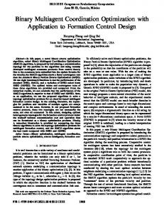
this d on the set of µ-memory strategy profiles. We denote by Coli (A) the i-th column of A, and |S| the cardinal number of set S (for a finite set, it is the number of the elements in S). Then the following proposition is an immediate consequence of the definition. Proposition 4.6: Let A, B ∈ Lk×kµ . Then |{i |Coli (A) 6= Coli (B) }| = d(A, B). (19) When µ = 1, we have more clear description for the geometric meaning of this distance. Now assume µ = 1 and L is given, the next action x(t + 1) can be determined from x(t), then we can draw a strategy dynamic graph to depict L. We give an example for this. Example 4.7: Assume a game consists of two players A and B. A has two actions and B has three actions, i.e., x1 ∈ ∆2 and x2 ∈ ∆3 . Setting x = x1 x2 , we assume the strategy profile is x(t + 1) = Lx(t) = δ6 [3, 4, 5, 2, 1, 3]x1 (t)x2 (t).

(20)

Note that δ61 ∼ (1, 1), δ62 ∼ (1, 2), δ63 ∼ (1, 3), δ64 ∼ (2, 1), δ65 ∼ (2, 2), δ66 ∼ (2, 3), according to (20) it is easy to draw the strategy dynamic graph as in Fig. 1. Fig. 1 Strategy Dynamic Graph

(1,1)

(2,1)

(1,2)

(2,2)

(1,3)

(2,3)

The following theorem shows the deep geometric meaning of the distance. Theorem 4.8: Assume µ = 1. Then the distance d(L1 , L2 ) between two strategy profiles is the number of different edges between the strategy dynamic graphs of L1 and L2 . Proof. In the strategy dynamic graph each node has exactly out-degree 1, that is, there is exactly one directed edge starting from each node. For a strategy profile L assume Coli (L) = δkj , then it means the strategy profile will lead x(t) = δki to x(t + 1) = δkj . That is, Coli (L) uniquely determines the edge starting from the node δki . The conclusion follows. 2 As for µ > 1 case, since x(t + 1) depends on µ historical strategy profiles, we define a path

number of different compounded edges between the strategy dynamic graphs of L1 and L2 . V. L OCAL NASH /S UB -NASH E QUILIBRIUMS µ Consider the set of µ-memory strategy profiles, S∞ . Let L0 ∈ Lk×kµ . ǫ ∈ Z+ be a positive integer. The ǫneighborhood of L0 is defined as

Bε (L0 ) = { L ∈ S µ | d(L, L0 ) ≤ ε} .

(21)

Definition 5.1: A strategy profile L0 is called a local Nash/sub-Nash equilibrium on Bǫ , if it is a Nash/sub-Nash equilibrium with respect to its ǫ-neighborhood. We explain the motivation for investigating local Nash/sub-Nash equilibriums. It was shown in [9] that the number of µ-member strategy profiles is µ

|Lk×kµ | = k (k ) .

(22)

It is clear that finding the Nash/sub-Nash equilibriums by exhaustive search is extremely difficult except some simplest cases. To find the Nash/sub-Nash solutions for a dynamic game, our idea is (1) Build a proper topological structure (metric) on the set of strategy profiles. This topology should be meaningful, which means the neighboring strategy profiles are essentially related. (2) Under this structure we can search a local Nash/sub-Nash solution by certain optimization process. In fact, (1) has been solved in previous section. As for (2) we may use hill climbing method. Then we propose the following algorithm. In the algorithm we consider a Nash equilibrium as a special sub-Nash equilibrium with tolerance ǫ = 0. In the following the sub-Nash equilibrium is either common sub-Nash one or mean sub-Nash one. Before stating the algorithm, we give some notations: (i) H: the set of historic strategy profiles, which have been used before. Denote by Hc = Lk×km \H. (ii) Lp the set of sub-Nash equilibriums, which are obtained from p-th iteration. (iii) Lp ∈ Lp , the strategy profile chosen from Lp for (p + 1)-th iteration. (iv) NLp : The neighborhood of Lp , NLp := { L ∈ Lk×kmu | d(L, Lp ) ≤ ε} . The default ǫ is ǫ = 1. Algorithm 5.2: • Step 0. Choose an initial strategy profile L0 , set H = {L0 }. • Step 1. On the neighbor NL0 of L0 search sub-Nash equilibrium(s), denoted as L1 = {L11 , L21 , · · · , Lk11 }.

x(t − µ + 1) → x(t − µ + 2) → · · · → x(t) → x(t + 1) as a compounded edge. The strategy dynamic graph of a µ-memory strategy profile consists of all such compounded edges. Then the following corollary is clear. Corollary 4.9: Assume µ > 1. Then the distance d(L1 , L2 ) between two µ-memory strategy profiles is the

5825

•

– If L0 ∈ L1 , choose L0 as a local sub-Nash equilibrium (the solution) and stop. – Else, if L1 ∩Hc = ∅, no local sub-Nash equilibrium is found (the algorithm fails) and stop. – Else, choose L1 ∈ L1 ∩ Hc , and add L1 to H. Step 2. On the neighbor NL1 of L1 search sub-Nash equilibrium(s), denoted as L2 = {L12 , L22 , · · · , Lk22 }.

• •

– If L1 ∈ L2 , choose L1 as a local sub-Nash equilibrium (the solution) and stop. – Else, if L2 ∩ Hc = ∅, go back to Step 1. – Else, choose L2 ∈ L1 ∩ Hc , and add L2 to H. ··· Step p. On the neighbor NLp−1 of Lp−1 search subNash equilibrium(s), denoted as Lp = {L1p , L2p , · · · , Lkpp }.

– If Lp−1 ∈ Lp , choose Lp−1 as a local sub-Nash equilibrium (the solution) and stop. – Else, if Lp ∩ Hc = ∅, go back to Step p-1. – Else, choose Lp ∈ Lp ∩ Hc , and add Lp to H. • ··· µ Remark 5.3: 1) Since |Lk×kµ | = k (k ) < ∞, the algorithm will terminate somewhere. 2) Only when the chosen optimal strategy profiles L0 , L1 , · · · , form a cycle, the algorithm fails. Otherwise, a local sub-Nash equilibrium can be obtained. Theoretically, we have no reason to claim that the algorithm will never fail. But in numerical computations, we did not have experience of failing. We give some examples to depict it. Example 5.4: Consider the infinitely repeated game of prisoners’ dilemma, the payoff bi-matrix is TABLE I PAYOFF BI - MATRIX P1 \P2 1 2

1 3,3 5,0

2 0,5 1,1

Choose L0 = δ4 [1 1 1 3], using Algorithm 5.2, we have L1 L2 L3 L4 L5 L6

= δ4 [1 4 1 3], = δ4 [1 3 1 3], = δ4 [1 3 4 3], = δ4 [3 3 4 3], = δ4 [3 3 4 2], = δ4 [3 4 4 2],

L7 = δ4 [4 4 4 2] L8 = δ4 [1 4 4 2] L9 = δ4 [2 4 4 2] L10 = δ4 [2 4 4 4] L11 = δ4 [1 4 4 4].

The algorithm terminates at k = 11, L11 is a locally Nash equilibrium, which is also a 1-memory Nash equilibrium [9]. The algorithm can not always find a Nash equilibrium, for example, let L0 = δ4 [2 1 2 3], then we can find a locally Nash equilibrium L = δ4 [1 4 2 1] which is not Nash equilibrium. VI. O PTIMIZATION OF M IXED - VALUE L OGICAL N ETWORKS

where xi ∈ Dki , i = 1, · · · , n; uj ∈ Drj , j = 1, · · · , m; fi , i = 1, · · · , n are logical functions. It is briefly denoted as X(t + 1) F (X(t), U (t)), Q Q= n m X(t) ∈ i=1 Dki , U (t) ∈ j=1 Drj .

(24)

Qn Let x(t) Q := ⋉ni=1 xi (t), u(t) := ⋉m i=1 ui (t), k := i=1 ki , m and r := j=1 rj . We can equivalently express (23) (equivalently, (24)) in an algebraic form as [5] x(t + 1) = Lu(t)x(t),

x ∈ ∆k , u ∈ ∆r

(25)

where L ∈ Lk×k+r is also called the transition matrix. Assume the performance criterion is T 1X c(x(t), u(t)), T →∞ T t=1

J(u) = lim

(26)

where c is a function from Dk+r to R. This criterion may be considered as for a particular player in game theory. Definition 6.1: Consider the mixed-value control network (23). Assume x0 = x(0) is given. The optimization problem with respect to criterion (26) is finding {u∗ (t)|t = 0, 1, 2, · · · }, such that J(u∗ ) ≥ J(u), ∀u. (27) We cite some basic results from [18], [24], [23], which are the starting point of the work in this section. The following result is from [18] and extended to general case by [24], [23]. Theorem 6.2: There exists an optimal trajectory, corresponding to the optimal control, which is periodic on statecontrol product space. The following result is from [24]. Theorem 6.3: The optimal control can be expressed as  u (t + 1) = g1 (x1 (t), · · · , xn (t), u1 (t), · · · , um (t))    1  u2 (t + 1) = g2 (x1 (t), · · · , xn (t), u1 (t), · · · , um (t)) ...     um (t + 1) = gm (x1 (t), · · · , xn (t), u1 (t), · · · , um (t)). (28) Remark 6.4: According to Theorem 6.3, we can combine (28) with (23) to get an overall system. It is easy to see that the overall system (23)-(28) is the same as (4) with µ = 1. But the control (strategy) considered in this section is initialvalue-depending. Recall the system (23). Its algebraic form is expressed as x(t + 1) = Lx(t)u(t),

(29)

where L ∈ Lk×kr . Similarly, the algebraic form of (28) is denoted as

The dynamics of a mixed-value logical control network is expressed as  x1 (t + 1) = f1 (x1 , · · · , xn , u1 , · · · , um )    x (t + 1) = f (x , · · · , x , u , · · · , u ) 2 2 1 n 1 m (23)  ···    xn (t + 1) = fn (x1 , · · · , xn , u1 , · · · , um ),

u(t + 1) = Gx(t)u(t),

(30)

where U ∈ Lr×kr . Multiplying both sides of (29) and (30) together yields

5826

x(t + 1)u(t + 1) = Lx(t)u(t)Gx(t)u(t) = L(Ikr ⊗ G)x(t)u(t)x(t)u(t) = L(I2n+m ⊗ G)Φx(t)u(t),

where

R EFERENCES

¡ 1 2 ¢ kr Φ = diag δkr , δkr , · · · , δkr .

Define w(t) = x(t)u(t), then we have

w(t + 1) = Ψ(G)w(t),

(31)

For every G, we can calculate Ψ(G), and then find the cycles of (31) for every initial u0 , thus by comparing the criterions we can find the optimal control. But in general, searching all G ∈ Lr×kr to find an optimal solution is unrealistic because of the computation complexity. Note that the method in [24] which search the optimal cycle of logical control network also has huge computation complexity. Again, at each step, we look for only a local optimal solution. That is, look for optimal solution G over a neighborhood NG0 := Bǫ (G0 ) = { G ∈ Lr×rk | d(G, G0 ) ≤ ε} . Set the default ǫ = 1. We propose the following algorithm. Algorithm 6.5: • Step 1: Choose a G0 ∈ L2m ×2m+n . • Step p: Find the best solutions over NGp−1 , say, p,kp

kp Gp = {(G1p , up,1 0 ), · · · , (Gp , u0

)}.

If there exists a Gip = Gp−1 , stop. Taking (Gp−1 , up,i 0 ) as the local optimal control. Else, choose Gp = G1p , continue. Example 6.6: Consider a Boolean network x(t + 1) = Lx(t)u(t), where L = δ2 [1 2 2 1]. Assume ′

c(x(t), u(t)) = u (t)

·

1 3

2 4

¸

x(t)

and x0 = δ22 , L = δ2 [1 2 2 1], x0 = δ22 . Choose G0 = δ2 [1 2 2 1], using algorithm 6.5 we can get that in step 1 G1 = {(δ2 [1 2 2 2], δ21 ), (δ2 [1 2 2 2], δ22 )}. We choose G1 = δ2 [1 2 2 2], then G2 = {(δ2 [1 2 2 2], δ21 ), (δ2 [1 2 2 2], δ22 ), (δ2 [2 2 2 2], δ21 ), (δ2 [2 2 2 2], δ22 )}. Thus, (δ2 [1 2 2 2], δ21 ) and (δ2 [1 2 2 2], δ22 ) are local optimal controls. We can check that they are also optimal controls.

[1] T. Akutsu, S. Miyano, S. Kuhara, Inferring qualitative relations in genetic networks and metabolic pathways, Bioinformatics, Vol. 16, 727-73, 2000. [2] R. Albert, A-L Barabasi, Dynamics of complex systems: scaling laws or the period of Boolean networks, Phys. Rev. Lett., Vol. 84, 56605663, 2000. [3] D. Cheng, Semi-tensor product of matrices and its applications — A survey, ICCM 2007, Vol. 3, 641-668, 2007. [4] D. Cheng, Input-state approach to Boolean networks, IEEE Trans. Neural Network, Vol. 20, No. 3, 512-521, 2009. [5] D. Cheng, H. Qi, Controllability and observability of Boolean networks, Automatica, Vol. 45, No. 7, 1659-1667, 2009. [6] D. Cheng, Z. Li, H. Qi, Realization of Boolean control networks, Automatica, Vol. 46, No. 1, 62-69, 2010. [7] D. Cheng, H. Qi, A linear representation of dynamics of Boolean networks, IEEE Trans. Aut. Contr., Vol. 55, No. 10, 2010. (to appear). [8] D. Cheng, H. Qi, Z. Li, J. Liu, Stability and stabilization of Boolean networks, Int. J. Robust Nonlin. Contr., 2010. (to appear) [9] D. Cheng, Y. Zhao, Z. Li, Sub-Nash solution to infinitely repeated games. (submitted to Int. J. Game Theory). [10] C. Farrow, J. Heidel, H. Maloney, J. Rogers, Scalar equations for synchronous Boolean networks with biological applications, IEEE Trans. Neural Networks, Vol. 15, No. 2, 348-354, 2004. [11] R. Gibbons, A Primer in Game Theory, FT Prentice Hall, London, 1992. [12] S. Huang, I. Ingber, Shape-dependent control of cell growth, differentiation, and apotosis: Switching between attractors in cell regulatory networks, Exp. Cell Res., Vol. 261, 91-103, 2000. [13] S. Huang, Regulation of cellular states in mammalian cells from a genomewide view, in Gene Regulation and Metabolism, J. ColladoVodes and R. Hofestadt, Eds. Cambridge, MA:MIT Press, 181-220, 2002. [14] S.A. Kauffman, Metabolic stability and epigenesis in randomly constructed genetic nets, J. Theoretical Biology, Vol. 22, 437-467, 1969. [15] S.A. Kauffman, The Origins of Order: Self-organization and Selection in Evolution, Oxford University Press, New York, 1993. [16] S.A. Kauffman, At Home in the Universe, Oxford University Press, New York, 1995. [17] Z. Li, D. Cheng, Algebraic Approach to Dynamics of Multi-valued Networks, Int. J. Bifurcat. Chaos, Vol. 20, No. 3, 561-582, 2010. [18] Y. Mu, L. Guo, Optimization and identification in a non-equilibrium dynamic game, Proc. CDC-CCC’09, 5750-5755, 2009. [19] M. Puterman, Markov Decision Processes: Discrete Stochastic Dynamic Programming, John Wiley & Sons, Inc., New York, 1994. [20] B. Samuelsson, C. Troein, Superpolynomial growth in the number of attractots in kayffman networks, Phys. Rev. Lett., Vol. 90, 90098701, 2003. [21] I. Shmulevich, R. Dougherty, S. Kim, W. Zhang, Probabilistic Boolean neworks: A rule-based uncertainty model for gene regulatory networks, Bioinformatics, Vol. 2, No. 18, 261-274, 2002. [22] F. Robert, Discrete Iterations, A Metric Study, Translated by J. Rokne, Springer-Verlag, Berlin, 1986. [23] Y. Zhao, D. Cheng, Optimal control of mix-valued logical control systems, Proc. CCC’10, 1618-1623, 2010. [24] Y. Zhao, D. Cheng, Optimal control of logical control networks, preprint. (submitted for pub)

VII. C ONCLUSION In this paper a metric was introduced to the set of strategy profiles of a dynamic game with finite memory. The geometric meaning of the metric was explained. Using it, the concept of local Nash/subNash equilibrium(s) was introduced and the geometric meaning was revealed. When the initial-value-independent strategy profiles for dynamic games were considered, a hill climbing algorithm was introduced to find the local Nash/sub-Nash equilibrium(s). As another application, the optimization of mixed-value logical control systems was investigated, and the algorithm is proposed to get local “best” initial-value-dependent strategy.

5827