The goal of a TD algorithm, run on M, is to distribute the tokens evenly among ..... We use the well-known MaxflowâMincut Theorem (see [15]). Let Vf be the.
Algorithmica (1996) 15: 413–427
Algorithmica ©
1996 Springer-Verlag New York Inc.
Strongly Adaptive Token Distribution1 F. Meyer auf der Heide,2 B. Oesterdiekhoff,2 and R. Wanka2 Abstract. The token distribution (TD) problem, an abstract static variant of load balancing, is defined as follows: let M be a (parallel processor) network with set P of processors. Initially, each processor P ∈ P has a certain amount l(P) of tokens. The goal of a TD algorithm, run on M, is to distribute the tokens evenly among the processors. In this paper we introduce the notion of strongly adaptive TD algorithms, i.e., algorithms whose running times come close to the best possible runtime, the off-line complexity of the TD problem, for each individual initial token distribution l. Until now, only weakly adaptive algorithms have been considered, where the running time is measured in terms of the maximum initial load max{l(P)|P ∈ P}. We design an almost optimal, strongly adaptive algorithm on mesh-connected networks of arbitrary dimension extended by a single 1-bit bus. This result shows that an on-line TD algorithm can come close to the optimal (off-line) bound for each individual initial load. Furthermore, we exactly characterize the off-line complexity of arbitrary initial token distributions on arbitrary networks. As an intermediate result, we design almost optimal weakly adaptive algorithms for TD on mesh-connected networks of arbitrary dimension. Key Words. Parallel algorithms, Token distribution.
1. Introduction. 1.1. Computation Model. The underlying parallel computation model is the (parallel processor) network. Such a network consists of a set of p processors, P = {P1 , . . . , Pp } pairs of which are connected via bidirectional links forming a communication graph M = (P, E) with E denoting the set of links. We identify the network with its communication graph. The network is assumed to be synchronized; in a computation step, each processor can do a constant amount of internal computation and can send a message to a neighboring processor. We demand that each processor can receive at most one message per step. 1.2. The Token Distribution Problem. Load balancing is one of the basic tasks to be performed in order to achieve efficient execution of parallel programs on a network: if a processor is overloaded with work during a computation, it tries to reduce its load by shifting part of it to less busy processors. The aim is to keep the load balanced among the processors. Token distribution (TD) is an abstraction of a static variant of load balancing. Initially each processor P has a number Pl(P) of tokens, i.e., the initial load is given by a function l: P → N. We refer to N = P∈P l(P) as the total load, to k = max{l(P)|P ∈ P} as the maximum load, and to N / p as the average load. 1 This research was partially supported by DFG-Forschergruppe “Effiziente Nutzung massiv paralleler Systeme, Teilprojekt 4,” by the ESPRIT Basic Research Action No. 7141 (ALCOM II), and by the Volkswagenstiftung. A preliminary version was presented at the 20th ICALP, 1993, see [9]. 2 Fachbereich Mathematik-Informatik and Heinz-Nixdorf-Institut, Universit¨ at-GH Paderborn, D-33095 Paderborn, Germany. {fmadh,brigitte,wanka}@uni-paderborn.de.
Received November 9, 1993; revised May 11, 1994, and August 21, 1994. Communicated by K. Mehlhorn.
414
F. Meyer auf der Heide, B. Oesterdiekhoff, and R. Wanka
The goal of token distribution is to distribute the tokens given by the initial load so that the final load of each processor is close to the average load. More specifically, a TD algorithm is δ-exact if finally no processor holds more than dN / pe + δ tokens. Furthermore, we denote the maximum load difference of the processors with discrepancy. 1.3. Complexity Measures of Token Distribution. In order to be able to measure the performance of a TD algorithm, we first introduce a quantity which is a lower bound on the running time of any TD algorithm on M with initial load l. For this purpose, we consider off-line algorithms for token distribution. In this case, with M, l given, we allow an arbitrarily complex preprocessing that can be executed without being added to the complexity and that produces a protocol for each processor telling, for each time t, whether and, if yes, where to send a token. We assume that a processor can send and receive one token per time step. The off-line complexity of the TD problem (M, l), the TD problem on M with initial load l, is T off (M; l, δ), the running time of a fastest δ-exact off-line TD algorithm. On-line algorithms are designed for a fixed network M, but do not allow any free preprocessing given an initial load l. Thus, a TD algorithm executes distribution steps, where each processor can send and receive one token, and computation steps, where computation and communication can take place (e.g., to gather information about the current load distribution). No tokens are moved in such a step. The on-line complexity of the TD problem (M, l) is T (M; l, δ), the running time of a fastest δ-exact on-line TD algorithm on M started with initial load l. All papers mentioned below consider the following adaptive complexity measure for TD on M: Tad (M; N , k, δ) = max{T (M; l, δ)|l has maximum load ≤ k and total load ≤ N }. In this paper we consider an even stronger version of adaptivity: we want to design online TD algorithms which come close to the performance of off-line algorithms of each individual initial load function, i.e., we design strongly adaptive TD algorithms, showing that their performance comes close to the lower bound, i.e., the off-line complexity. The strongly adaptive complexity is the running time of a fastest δ-exact on-line TD algorithm depending on the off-line complexity T off (M; l, δ), the network M, and the maximum load k of the individual load l. We assume that the total load N is initially known to all processors. 1.4. Known Results About Token Distribution. The token distribution problem was introduced by Peleg and Upfal [10]. For arbitrary networks M with p processors and total load N = p, the same authors show in [11] that, for all k ≥ 2, Tad (M; p, k, 0) = O( p)
and
Tad (M; p, k, 0) = Ä(k + diam(M)),
with diam(M) denoting the diameter of M.
Strongly Adaptive Token Distribution
415
Matching upper bounds are shown in [11], by Herley [4], and by Broder et al. [3] for certain classes K of expander-related, bounded-degree, low-diameter networks, i.e., Tad (M; p, k, O(1)) = O(k + log p) for all M ∈ K. Aiello et al. [1] analyze a very simple algorithm for arbitrary graphs and show by using advanced and elegant techniques that, for constant-degree graphs G µ with p processors and expansion µ, ¶¶ µ ¶ µ µ k· p−N 1 log p =O log(k · p − N ) . Tad G µ ; N , k, O µ p·µ Plaxton [12] investigates the TD problem on the d-dimensional hypercube Q d . He shows that, for k ≥ 2 · N / p, à Tad (Q d ; N , k, 0) = Ä k ·
s d d + log(k/N )
!
√ and Tad (Q d ; poly( p), k, 0) = O(k d + d 2 ). Werchner [16] deals with certain TD problems on Q d . By carefully analyzing expansion properties of Q d , he shows that Tad (Q d ; k · p 1/2−Ä(1) , k, 0) = O(k + d 2 · log d). J´aJ´a and Ryu [5] investigate the TD problem for the cube-connected cycles network, shuffle-exchange network, and the butterfly network. Qiu and Akl [13] do so for the star and pancake networks. Makedon √ and Symvonis [8] address the many-to-one routing problem on the two√ dimensional p-sided mesh M( p, 2). Their results can easily be modified to show that p p Tad (M( p, 2); p, k, 0) = 2( k · p) . Very recently, the many-to-one routing problem for higher-dimensional meshes was investigated in [14], where similar bounds are shown. A further approach to the TD problem is counting networks introduced by Aspnes et al. [2] and improved by Klugerman and Plaxton [6], where circuits for the TD problem are constructed similar to sorting circuits. 1.5. New Results About Token Distribution. In this paper we characterize almost exactly the off-line complexity of TD. Furthermore, we consider TD on the d-dimensional n-sided mesh-connected network M(n, d) and characterize its adaptive TD complexity up to a factor of O(d 2 ) (resp. O(d · 2d ) if the maximum load is small). Finally, we present a strongly adaptive algorithm for TD on M(n, d) which only differs by a factor of O(d 3 · log k) (resp. O(d · 2d + d 3 · log k) if the maximum load is small) from the off-line bound. More specifically, we prove: THEOREM 1 (Off-line Complexity of TD).
Let M be a network and let l be an initial
416
F. Meyer auf der Heide, B. Oesterdiekhoff, and R. Wanka
P load. For X ⊆ P, let I (X ) := P∈X l(P) be the load of X , and let N = I (P). match(X ) denotes the cardinality of a maximum matching between X and P \ X . ' & I (X ) − dN / pe · |X | off (a) . T (M; l, 0) ≥ max ∅$X $P match(X ) & (b)
T (M; l, 1) ≤ max off
∅$X $P
' I (X ) − dN / pe · |X | . match(X )
Thus, we obtain an exact characterization of the off-line complexity of TD with the restriction that the upper bound only holds if we allow the final maximum load to be one token larger than desired. The following observation shows, if we allow only ' & I (X ) − dN / pe · |X | max ∅$X $P match(X ) steps, that TD cannot be solved 0-exactly. OBSERVATION 1. properties:
There is an infinite family of TD problems (M, l) with the following
& k ≤ max
∅$X $P
N = p, I (X ) − dN / pe · |X | match(X )
and T off (M; l, 0) ≥ T + 2 ·
√
' = 12 p + 1 =: T,
T − 1 − 4.
THEOREM 2 (Weakly Adaptive Complexity of TD on Meshes). √ d (a) For k ≥ 2 · (N /n d ), Tad (M(n, d);√N , k, 0) = Ä((1/d) · N · k d−1 ). d (b) Tad (M(n, d); N , k, 0) = O(2d · N · k d−1 + 2d · n). √ d For k ≥ 2 · (N /n d ), Tad (M(n, d); N , k, 0) = O(d · N · k d−1 + d 2 · n). This theorem extends the result of [8] mentioned above. We use its basic ideas, but have to add further techniques to generalize for arbitrary total load and arbitrary dimension. Note that, for constant d, the bounds in Theorem 2 match. We extend our underlying parallel computation model by a global bus capable of storing one bit. Each processor is able to write on and to read from this bus in one time step. By using the weakly adaptive algorithms as subroutines, we show the following main result of this paper. THEOREM 3 (Strongly Adaptive Complexity of TD on Meshes). T (M(n, d); l, 1) = O((d · 2d + d 3 · log k) · T off (M(n, d), l, 0)). For k ≥ 2 · (N /n d ), T (M(n, d); l, 1) = O((d 3 · log k) · T off (M(n, d), l, 0)) for each individual load l with maximum load k. This result shows that an on-line TD algorithm can come close to the optimal (off-line) bound for each individual initial load.
Strongly Adaptive Token Distribution
417
2. The Off-line Complexity of Token Distribution THEOREM 1 (Off-line Complexity P of TD). Let M be a network, and let l be an initial load. For X ⊆ P, let I (X ) := P∈X l(P) be the load of X , and let N = I (P). match(X ) denotes the cardinality of a maximum matching between X and P \ X . ' & I (X ) − dN / pe · |X | off (a) . T (M; l, 0) ≥ max ∅$X $P match(X ) & (b)
T off (M; l, 1) ≤ max
∅$X $P
' I (X ) − dN / pe · |X | . match(X )
2.1. Off-line Lower Bound. The lower bound is based on expansion properties of M like Plaxton’s lower bound [12]. It is similar to that mentioned by Peleg and Upfal [11]. PROOF OF THEOREM 1(a). Consider an arbitrary set X of processors, ∅ $ X $ P. Initially, X contains I (X ) tokens, finally at most dN / pe · |X |. Thus, I (X ) − dN / pe · |X | tokens have to leave X . At most match(X ) tokens can leave X per time step. Thus, any solution to the TD problem requires at least max∅$X $P d(I (X )−dN / pe·|X |)/match(X )e distribution steps. In what follows, we show that this bound is tight for arbitrary networks, if we allow preprocessing, and if some processors may eventually hold one token more than the average load. Note that, in this case, the diameter of M does not influence the off-line running time in the following sense. Consider a graph consisting of K p/2 , the complete graph of 12 p nodes, and a linear array of length 12 p where one of the endnodes of the array is connected to an arbitrary node of K p/2 . The diameter of the graph is 12 p + 1 = 2( p). If we have p tokens only distributed on K p/2 with initial maximum load k = O(log p), these tokens can be distributed on K p/2 in O(log p) steps so that finally each processor has exactly two tokens, i.e., one token more than the average load. However, if it is required that each processor holds exactly one token, each algorithm needs at least Ä( p) steps for the given problem. 2.2. An Almost Optimal Off-line Algorithm PROOF OF THEOREM 1(b). To prove the theorem, we use a novel approach. We transform the TD problem on M = (P, E) with initial load l and desired final maximum load m into a maximum flow problem on a directed flow graph G f (M, l, t, m) (or G f for short). The parameter t stands for the running time we allow to solve the TD problem. For the terminology of network flow methods, see, e.g., [15]. An example for the transformation of the linear array M(3, 1) of length 3 with initial load l, l(P1 ) = 4, l(P2 ) = 3, l(P3 ) = 5, into the flow graph G f (M(3, 1), l, 2, 4) is given in Figure 1. G f consists of main levels V0 , . . . , Vt and, associated with them, helping levels bt−1 , V e1 , . . . , V et . Each level consists of copies of all processors of M. The flow b0 , . . . , V V from the source q to a vertex in Vi represents the load of the corresponding processor
418
F. Meyer auf der Heide, B. Oesterdiekhoff, and R. Wanka
Fig. 1. Transformation of (M(3, 1), l) into the flow-graph G f (M(3, 1), l, 2, 4). The four marked nodes form a cut C with cap(C) = 13.
of M after i distribution steps of a possible TD algorithm. In particular, a path between two main levels Vi and Vi+1 models a single distribution step. To establish the initial distribution of tokens, we have edges from the source q to the vertices in V0 , where the capacities are chosen with respect to the initial load l. As the vertices in Vt represent the token distribution at the end of a possible TD algorithm, these vertices are connected to the sink s via edges with capacity m. bi To model the constraints of a single distribution step, we use two helping levels V e and Vi+1 between each Vi and Vi+1 , i ∈ {0, . . . , t − 1}. The reason is that we have to take care of the following mode of communication among processors as described in the Introduction: 1. Each processor can send at most one token per time step (ensured by the edges with bi ). capacity 1 between Vi and V 2. Each processor can receive at most one token per time step (ensured by the edges ei+1 and Vi+1 ). with capacity 1 between V 3. Each processor holds the tokens not transmitted (ensured by the edges with infinite capacity between Vi and Vi+1 ). See Figure 1 for the details of realizing 1–3. Finally, the helping levels are connected with respect to the links of M by edges with capacity ∞. As all capacities are integers, the Integrality Theorem (see [15]) ensures that there is a maximum flow such that all flows along all edges are integers. Therefore, if there is a maximum flow with value N in G f , the N tokens can be redistributed among M in t steps, so that eventually the maximum number of tokens in any processor is at most m. Of course, we want m = dN / pe (average load) and t as small as possible. The following lemma implies Theorem 1(b). LEMMA 1.
The value of a maximum flow on G f = G f (M, l, T, dN / pe + 1) is N , if & T = max
∅$X $P
' I (X ) − dN / pe · |X | . match(X )
Strongly Adaptive Token Distribution
419
PROOF. We use the well-known Maxflow–Mincut Theorem (see [15]). Let V f be the vertices and c the capacities in G f . Let C ⊂ V f be an arbitrary (q, s)-cut in G f , i.e., q ∈ C and s ∈/ C (see Figure 1). LetP out(C) denote the set of edges from nodes in C to nodes in V f \ C, and cap(C) = e∈out(C) c(e) the capacity of C. We show that cap(C) ≥ N . For u ∈ P, let u i ∈ Vi denote the copy of u in Vi . Let Ci = C ∩ Vi , orig(Ci ) = {u ∈ V |u i ∈ Ci }. If C0 = ∅, or Ct = Vt , or out(C) contains an edge with infinite capacity, cap(C) ≥ N is obviously true. Now assume that C0 6= ∅, Ct 6= Vt , and out(C) contains none of the edges with infinite capacity. As a consequence, we have Ci+1 ⊇ {u i+1 |u i ∈ Ci }. If Ci+1 = {u i+1 |u i ∈ Ci }, the subgraph induced by Vi , Vi+1 , and the corresponding helping levels contributes at least match(orig(Ci )) to cap(C), because a maximum matching between orig(Ci ) and orig(Vi \ Ci ) corresponds directly to a system of vertex-disjoint paths between Vi and Vi+1 , each path leaving C. That means for each edge {u, v} of the maximum matching between orig(Ci ) and orig(Vi \ Ci ), u i ∈ Ci and vi+1 ∈/ Ci+1 . Thus, there is a cut of at least 1 on the path between u i and vi+1 . If Ci+1 % {u i+1 |u i ∈ Ci }, each vertex in Ci+1 \ {u i+1 |u i ∈ Ci } decreases the capacity match(orig(Ci )) by at most 1 because the paths to them do not leave C. Thus, the contribution of the edges between Vi and Vi+1 to cap(C) is at least match(orig(Ci )) − (|Ci+1 | − |Ci |) for all i < T . Using this fact and that I (orig(Ci )) − dN / pe · |Ci | match(orig(Ci ))
T ≥
for all i,
we have the following estimation for cap(C): X
cap(C) =
l(u) +
u∈orig(V0 \C0 )
µ»
+
N p
¼
¶ match(orig(Ci )) − (|Ci+1 | − |Ci |)
T −1 µ X i=0
+ 1 · |C T | »
= I (orig(V0 \C0 )) + |C0 | + » ≥ I (orig(V0 \C0 )) + |C0 | +
N p N p
¼ · |C T | + ¼
T −1 X
match(orig(Ci ))
i=0
· |C T | + T · match(orig(C j )) » ¼ N · (|C T | − |C j |) ≥ I (orig(V0 \ C0 )) + I (orig(C j )) +|C0 | + | | {z } {z } p ≥N
≥0
≥ N, where j is such that match(orig(C j )) = min{match(orig(Ci ))|0 ≤ i ≤ T − 1}. Thus, C = {q} is a minimum cut with cap(C) = N .
420
F. Meyer auf der Heide, B. Oesterdiekhoff, and R. Wanka
Fig. 2. 0-exact TD requires more than T steps.
There is an infinite family of TD problems (M, l) with the following
OBSERVATION 1. properties:
& k ≤ max
∅$X $P
N = p, I (X ) − dN / pe · |X | match(X )
and T off (M; l, 0) ≥ T + 2 ·
√
' = 12 p + 1 =: T,
T − 1 − 4.
PROOF. Consider the network M shown in Figure 2 and the given initial load. K p/2 denotes the complete network consisting of 12 p processors. For this TD problem, we have ' & I (X ) − dN / pe · |X | = 12 p + 1 T = max ∅$X $P match(X ) (see the marked region). Because of the diameter of the marked region, at least q 1 + 2 · 12 p − 4 distribution steps are necessary.
1 2
p+
3. The Adaptive Complexity of Token Distribution on Meshes. THEOREM 2 (Weakly Adaptive Complexity of TD on Meshes). √ d (a) For k ≥ 2 · (N /n d ), Tad (M(n, d);√N , k, 0) = Ä((1/d) · N · k d−1 ). d d d d−1 + 2 · n). (b) Tad (M(n, d); N , k, 0) = O(2 · N · k √ d For k ≥ 2 · (N /n d ), Tad (M(n, d); N , k, 0) = O(d · N · k d−1 + d 2 · n). 3.1. Lower Bound PROOF OF THEOREM 2(a). We construct a poor input for the d-dimensional n-sided mesh M(n, d) as follows: Concentrate all tokens in a corner region of M(n, d) that
Strongly Adaptive Token Distribution
421
Fig. 3. All tokens are located at a corner of the mesh.
is isomorphic to M((N /k)1/d , d). (The situations for d = 2 and d = 3 are shown in Figure 3). This corner region has d · (N /k)(d−1)/d outgoing links. Arguing as in the proof of Theorem 1(a), any solution to the problem described above requires at least ¶ 1 √ N d · · N · k d−1 1− d n ·k d √ 1 1 d ≥ · · N · k d−1 2 d µ ¶ 1 √ d · N · k d−1 = Ä d
N − (N /n d ) · (N /k) = d · (N /k)(d−1)/d
µ
distribution steps, if k ≥ 2 · (N /n d ). Note that the condition k ≥ 2 · (N /n d ) is true for each TD problem on M(n, d) with total load N = n d . 3.2. Adaptive Algorithm √ d PROOF OF THEOREM 2(b). We first present a TD algorithm requiring O(2d ·( N · k d−1 + n)) steps. Note that this is optimal when d is constant. Concluding this section, we present an algorithm that is faster for the case that k ≥ 2 · (N /n d ). Let M1 , M2 , . . . , Mn be a partition of M(n, d) into n copies of M(n, d − 1), and let A1 , . . . , An d−1 be a partition into n d−1 linear arrays of length n where each vertex of an array belongs to a different Mr . The partition of M(n, d) into M1 , M2 , . . . , Mn and one As is shown in Figure 4. The following algorithm, started on M(n, d), generates a distribution with discrepancy 1. Note that such a distribution is 0-exact.
422
F. Meyer auf der Heide, B. Oesterdiekhoff, and R. Wanka
Fig. 4. Partition of M(n, d).
TD algorithm if d = 1 then 1. Distribute the tokens with discrepancy 1. if d > 1 then √ d 2. In each Mr , color min{ar , N d−1 · k} arbitrary tokens of the ar tokens in Mr black, and all remaining tokens white. 3. Recursively distribute the black tokens in each Mr with discrepancy 1. 4. Let kr be such that each processor in Mr contains kr or kr + 1 black tokens. Select kr of the black tokens in each processor of Mr . 5. Distribute the selected black tokens in each As with discrepancy 1. Comment: Note that the current distribution of the black tokens has overall discrepancy 2. 6. Distribute the white tokens in each As with discrepancy 1. 7. Let h s be such that each processor in As contains h s or h s + 1 white tokens. Select h s of the white tokens in each processor of As . 8. Recursively distribute the selected white tokens in each Mr with discrepancy 1. Comment: Note that the current distribution of the white tokens has overall discrepancy 2. Thus, the current distribution of all tokens has discrepancy 4. 9. Distribute the tokens in M(n, d), so that the discrepancy decreases to 1. algorithm solves each TD problem on M(n, d) with maximum LEMMA 2. The above √ d load k in O(2d · ( N · k d−1 + n)) steps with discrepancy 1. PROOF. (d = 1) Obviously, Step 1 can be executed in time O(N + n) (see [7]). (d > 1) The method of the algorithm is to split up the tokens into two sets and to balance one set at first in each Mr and then across each As and the other set at first across each As and then in each Mr . √ d In Step 2 we choose at most N d−1 · k black tokens and the rest of tokens are white, because this splitting guarantees that the time complexity for distributing the tokens in the (d − 1)-dimensional mesh Mr (Steps 3 and 8) is not too large. This splitting for the
Strongly Adaptive Token Distribution
423
case d = 2 and N = n 2 is used by Makedon and Symvonis [8] for many-to-one routing similarly. To execute Step 2, the tokens in each Mr are counted first. Then each processor knows how many of its at most k tokens it has to color black. In order to count the tokens, a prefix computation and a broadcast have to be done on a d-dimensional n-sided mesh. Both of these computations can be realized in O(d · n) steps by running d phases in each phase communicating on linear arrays of n processors. For these procedures, see [7]. √ d Thus, Step 2 requires√O(d · n + k) = O(d · n + N · k d−1 ) steps. d each Mr will be balanced with discrepIn Step 3 at most N d−1 · k black tokens in √ d ancy 1. By√inductive assumption, balancing N d−1 · k black tokens in Step 3 needs d O(2d−1 · ( N · k d−1 + n)) steps. In order to do Step 4, the value kr has to be known by each processor of Mr . Obviously, this can be done in O(d · n) steps by a prefix computation and a broadcast. Since the numbers of selected black tokens are the same √ in each As and there are d ≤ N · k d−1 selected black exactly N tokens in the mesh, there are at most N /n d−1 √ d in Step 5 requires O( N · k d−1 + n) time steps. tokens in every As . Thus, balancing √ d Since in each Mr up to N d−1 · k tokens √ are black, and since there are exactly d N tokens in the mesh, there are less than N / N d−1 · k = (N /k)1/d submeshes Mr containing white tokens. Thus, the total number of white tokens in each As is at most √ √ d d (N /k)1/d · k = N · k d−1 . Thus, Step 6 requires O( N · k d−1 + n) steps. Step 7 can be done in the same way as Step 4. Since the √ number of selected white d tokens are the same in each Mr , there are at most N /n ≤ N√d−1 · k selected white d tokens in each Mr , after Step 7. Thus, Step 8 requires O(2d−1 · ( N · k d−1 + n)) steps. In subsection 3.4.3 of [7], a monotone routing algorithm on d-dimensional hypercubes requiring O(d) steps is described. It can easily be generalized for meshes, needing O(d · n) steps on M(n, d). In Step 9 we redistribute the tokens in at most three phases, each phase reducing discrepancy by at least 1, performing monotone routing. Thus, Step 9 requires O(d · n) steps. √ d Altogether, the TD algorithm requires O(2d · ( N · k d−1 + n)) steps. For completeness, we present an adaptive TD algorithm achieving a better perfor√ d mance for a large maximum load, i.e., k ≥ 2·(N /n d ). It requires O(d · N · k d−1 +d 2 ·n) steps. Note that the condition k ≥ 2 · (N /n d ) is always true for TD problems with total load N = n d . Faster TD algorithm if d = 1 then 1. Distribute the tokens with discrepancy 1. if d > 1 then √ √ √ d 2. In each Mr , color min{ar , (( d 2−1)/ d 2) N d−1 · k} arbitrary tokens of the ar tokens in Mr black, and the remaining tokens white. 3. Distribute the white tokens in each As with discrepancy 1. 4. Let ks be such that each processor in As contains ks or ks + 1 white tokens. Select ks of the white tokens in each processor of As .
424
F. Meyer auf der Heide, B. Oesterdiekhoff, and R. Wanka
5. Recursively distribute the black tokens together with the selected white tokens in each Mr with discrepancy 1. 6. Let h r be such that each processor in Mr contains exactly h r , h r + 1, or h r + 2 tokens. Select h r of the tokens in each processor of Mr . 7. Distribute the selected tokens in each As with discrepancy 1. Comment: Note, the current distribution has discrepancy at most 3. 8. Distribute the tokens in M(n, d), so that the discrepancy is reduced to 1. The splitting into black and white tokens in Step 2 and the condition k ≥ 2 · (N /n d ) guarantee that the time complexity for distributing the tokens in Step 5 is not too large. By methods similar to those used in the proof of Lemma 2, the correctness and the time complexity of the above algorithm can be proved. Thus, Theorem 2(b) is proved.
4. The Strongly Adaptive Complexity of Token Distribution on Meshes THEOREM 3 (Strongly Adaptive Complexity of TD on Meshes). T (M(n, d); l, 1) = O((d · 2d + d 3 · log k) · T off (M(n, d), l, 0)). For k ≥ 2 · (N /n d ), T (M(n, d); l, 1) = O((d 3 · log k) · T off (M(n, d), l, 0)) for each individual load l with maximum load k.
3.2 it is shown that the (adaptive) complexity of the TD problem on PROOF. In Section √ d + n)), and for the case k ≥ 2 · (N /n d ) the complexity M(n, d) is O(2d · ( N · k d−1 √ d 2 can be improved to O(d · ( N · k d−1 + n)). Let T := T off (M(n, d), l, 0) be the offline complexity of the TD problem on M(n, d). Now we present a strongly adaptive algorithm solving the problem 1-exactly in O((d · 2d + d 3 · log k) · T ) steps and in O(d 3 · log k · T ) steps, if k ≥ 2 · N /n d , respectively. For that purpose, we partition M(n, d) into submeshes S(2dT, d) that are isomorphic to M(2dT, d). For example, we have illustrated such partitionings for d = 2 and d = 3, respectively, in Figure 5. The following lemma is the key observation for our method. It shows that if we solve the TD problem locally in each S(2dT, d), then the whole M(n, d) is balanced 1-exactly.
Fig. 5. Partitioning into submeshes.
Strongly Adaptive Token Distribution
425
LEMMA 3. Let S be an arbitrary submesh isomorphic to M(m, d) in M(n, d). Let L be the load of an arbitrary processor in S after balancing S. Then bbN /n d c − 2dT /mc ≤ L ≤ ddN /n d e + 2dT /me. PROOF. Let P be the total number of tokens initially located in an arbitrary submesh S of M(n, d). T is the real off-line complexity for solving the TD problem on M with initial load l 0-exactly. Thus, an optimal off-line algorithm balances during its execution on M(n, d) each S in T off-line steps. At most 2d · m d−1 tokens can leave S per time step, and at most dN /n d e · m d tokens may be in S after T time steps. Thus, P − 2dT · m d−1 ≤ dN /n d e · m d . Analogously, at most 2d · m d−1 tokens can enter S per time step, and at least bN /n d c · m d tokens must be in S after T time steps. Thus, P + 2dT · m d−1 ≥ bN /n d c · m d . After balancing each S, either L = bP/m d c or L = dP/m d e. The estimation for L is concluded directly. By Lemma 3, to solve the TD problem on M(n, d) 1-exactly, it is sufficient to solve the problem locally in each S(2dT, d). Here, the weakly adaptive algorithm described in Section 3.2 could be used locally. However, this direct application results in a running time that becomes quite large. Therefore, we use a more complicated procedure to solve the TD on M(n, d) 1-exactly, which is described in the following algorithm. Algorithm Local-TD (T ) 1. For each S(2dT, d): Determine the local maximum load ks and broadcast this value to all processors in S(2dT, d). 2. Consider a partition of each S(2dT, d) into submeshes S(2 · (2dT /ks ), d). Balance the tokens in each S(2 · (2dT /ks ), d) with discrepancy 1 by using one of the weakly adaptive algorithms described in Section 3.2. 3. for l := 1 to log ks − 1 do Combine 2d neighboring balanced S(2l · (2dT /ks ), d) to one S(2l+1 · (2dT /ks ), d) and reduce the discrepancy between all S(2l · (2dT /ks ), d) of each S(2l+1 · (2dT /ks ), d) in the following way: (a) for p := 0 to d − 1 do Determine the discrepancy between the two S(2l · (2dT /ks ), d) neighbored in dimension p, and reduce the discrepancy between these two submeshes to at most 2. Comment: After (a) is executed, the discrepancy in each S(2l+1 · (2dT /ks ), d) is at most d + 1. (b) for p := d downto 1 do Distribute the tokens in each S(2l+1 · (2dT /ks ), d), so that the discrepancy is decreased to at most p. LEMMA 4. Local-TD (T ) solves the TD problem on M(n, d) 1-exactly in O((d · 2d + d 3 · log k) · T ) steps and in O(d 3 · log k · T ) steps, if k ≥ 2 · (N /n d ), respectively.
426
F. Meyer auf der Heide, B. Oesterdiekhoff, and R. Wanka
PROOF. To execute Phase 1 a prefix computation and a broadcast have to be performed on a d-dimensional 2dT -sided mesh. Both of these computations can be realized in O(d 2 · T ) steps by running d phases in each phase operating on linear arrays of length 2dT . Since in each S(2 · (2dT /ks ), d) the maximum load is at most ks , and since the total number of tokens is at most ks · (2 · (2dT /ks ))d , the (adaptive) algorithm in Phase 2 requires O(d · 2d · T ) steps and O(d 3 · T ) steps, if k ≥ 2 · (N /n d ), respectively. Because of Lemma 3, we know that when pass l of the loop in Phase 3 is executed, the load of an arbitrary processor in each S(2l+1 · (2dT /ks ), d) is at least bbN /n d c − ks /2l+1 c and at most ddN /n d e + ks /2l+1 e. Hence, the discrepancy at the beginning of pass l is O(ks /2l ). Determining the discrepancy in Phase 3(a) can be done in O(d 2 · T ) steps in the same way as in Phase 1. Balancing in Phase 3(a) can be done by moving one token of each processor in S(2l · (2dT /ks ), d) to the corresponding processor in the neighbored S(2l · (2dT /ks ), d). Since the discrepancy is at most O(ks /2l ), balancing in Phase 3(a) needs O(d · T ) steps. Thus, Phase 3(a) requires O(d 3 · T ) steps. The distribution of tokens in Phase 3(b) in order to decrease the discrepancy can be implemented in the same way as in the algorithms in Section 3.2. Hence, Phase 3(b) needs O(d 3 · T ) steps. Thus, Phase 3 requires O(d 3 · log k · T ) steps. In the above algorithm we have assumed that the value of T is known by each processor in advance. In order to avoid this, we extend our network model by a global bus capable of storing one bit. Each processor is able to write on and to read from this bus in one time step. If the processors write different values, then the bus receives the logical AND of these values. Although the modified model does not rigorously fit into the fixed-connection network model, it is simple to realize in practice. The following algorithm solves the TD problem on M(n, d) 1-exactly in O((d · 2d + d 3 · log k) · T ) and in O(d 3 · log k · T ) steps, if k ≥ 2 · (N /n d ), respectively, without knowing the value of T in advance by using the modified network model. Algorithm TD t := 1. Do • t := 2 · t. • Local-TD (t). • Each processor P with load L P writes the following bit on the bus: » ¼ ¹ º N N − 1 ≤ LP ≤ + 1, 1 if d bus := n nd 0 otherwise. until bus = 1. Note that each processor has to know the total number N of tokens. LEMMA 5. Algorithm TD solves the token distribution problem on M(n, d) 1-exactly in O((d · 2d + d 3 · log k) · T ) steps and in O(d 3 · log k · T ), if k ≥ 2 · N /n d , respectively.
Strongly Adaptive Token Distribution
427
PROOF. In TD the algorithm Local-TD is started for t = 2, t = 22 , . . . , t = 2dlog T e . Pdlog T e Thus, TD requires i=1 O((d · 2d + d 3 · log k) · 2i ) = O((d · 2d + d 3 · log k) · T ) Pdlog T e time steps and O(d 3 · log k · 2i ) = O(d 3 · log k · T ) time steps, respeci=1 tively. This concludes the proof of Theorem 3. Note that with O(d · n · log T ) extra time, the additional global bus may be eliminated.
References [1] [2] [3] [4] [5] [6] [7] [8] [9] [10] [11] [12] [13] [14] [15] [16]
W. Aiello, B. Awerbuch, B. Maggs, and S. Rao. Approximate load balancing on dynamic asynchronous networks. Proceedings of the 25th ACM STOC, 1993, pp. 632–641. J. Aspnes, M. Herlihy, and N. Shavit. Counting networks and multi-processor coordination. Proceedings of the 23rd ACM STOC, 1991, pp. 348–350. A. Z. Broder, A. M. Frieze, E. Shamir, and E. Upfal. Near-perfect token distribution. Proceedings of the 19th ICALP, 1992, pp. 308–317. K. T. Herley. A note on the token distribution problem. Inform. Process. Lett., 38:329–334, 1991. J. J´aJ´a and K. W. Ryu. Load balancing and routing on the hypercube and related networks. J. Parallel Distrib. Comput., 14:431–435, 1992. M. Klugerman and C. G. Plaxton. Small-depth counting networks. Proceedings of the 24th ACM STOC, 1992, pp. 417–428. F. T. Leighton. Introduction to Parallel Algorithms and Architectures: Arrays, Trees, Hypercubes. Morgan Kaufmann, San Mateo, CA, 1992. F. Makedon and A. Symvonis. Optimal algorithms for the many-to-one routing problem on twodimensional meshes. Microprocessors and Microsystems, 17:361–367, 1993. F. Meyer auf der Heide, B. Oesterdiekhoff, and R. Wanka. Strongly adaptive token distribution. Proceedings of the 20th ICALP, 1993, pp. 398–409. D. Peleg and E. Upfal. The generalized packet routing problem. Theoret. Comput. Sci., 53:281–293, 1987. D. Peleg and E. Upfal. The token distribution problem. SIAM J. Comput., 18:229–243, 1989. C. G. Plaxton. Load balancing, selection and sorting on the hypercube. In Proceedings of the ACM SPAA, 1989, pp. 64–73. K. Qiu and S. G. Akl. Load balancing, selection, and sorting on the star and pancake interconnection networks. J. Par. Alg. Appl., 2:27–42, 1994. J. F. Sibeyn and M. Kaufmann. Deterministic 1-k-routing on meshes. Proceedings of the 11th STACS, 1994, pp. 237–248. R. E. Tarjan. Data Structures and Network Algorithms. Society for Industrial and Applied Mathematics, Philadelphia, PA, 1983. R. Werchner. Balancieren und Selection auf Expandern und auf dem Hyperw¨urfel. Diplomarbeit, J. W. Goethe-Universit¨at, Frankfurt, Jan. 1991 (in German).