INTRODUCTION. The truncated Volterra model has been the most popular in use since it can represent any nonlinear system time invariant with fading memory ...
9th International conference on Sciences and Techniques of Automatic control & computer engineering
Structure Identification of Volterra Models using Crosscumulants for Gaussian, PAM2 and QPSK input H. Mathlouthi(1), K. Abderrahim(1), F. Msahli(2) and G. Favier(3) (1) National School of Engineers of Gabès, Route de Medenine 6029 Gabès, Tunisie. (2) National School of Engineers of Monastir, Avenue Ibn Jazzar, 5019, Monastir, Tunisia. (3) I3S Laboratory, UNSA/CNRS, 2000 Route des Lucioles, Sophia-Antipolis, Biot, France.
Abstract: In this paper, we address the problem of structure identification of Volterra models. It consists in estimating the model order and the memory length of each kernel. Three methods based on input-output crosscumulants are developed. Simulations are performed on four models having different orders and kernel memory lengths to illustrate the performance of the proposed methods. Keywords: Structure identification, Volterra model, Volterra model Order, Kernel Memory Length, Crosscumulant,
1. INTRODUCTION The truncated Volterra model has been the most popular in use since it can represent any nonlinear system time invariant with fading memory [1]-[5]. Moreover, the parameters of this model are linearly related to the output which allows the extension of some results of linear systems to nonlinear ones. For these reasons, the truncated Volterra model has found applications in many fields such as signal processing and control. For the identification of truncated Volterra model, two main problems must be considered such as: identification of the model kernels and identification of the model structure defined by the model order and the kernel memory lengths. Several methods have been proposed in the literature for the identification of the kernels of Volterra model [6][11]. For the sake of simplicity, these methods assume that the model structure (model order and the memory length of each kernel) is a priori known or chosen arbitrary [6]-[11]. However, successful identification of Volterra parameters depends on the knowledge of the correct structure parameters. Consequently, the structure identification is one of the most difficult problems that represent an area of research to which few efforts have been devoted in the past. This paper addresses the problem of Volterra system structure identification based on crosscumulants. Three types of input sequence are considered: Gaussian input, binary symmetric input (PAM2) and Quadrature Phase Shift Keying (QPSK) input. In fact, we propose an algorithm for each type of input sequence that exploits the input statistics characteristics. This paper is organized as follows. Section 2 presents the model and its assumptions. Section 3 proposes the new algorithms. Results of simulations are presented in the last section. 2. PROBLEM FORMULATION In the following section, we address the problem of estimating the order and the kernel memory lengths of a discrete, causal stationary Volterra system described by: STA'2008-DIS-491, pages 1-9 Academic Publication Center of Tunis, Tunisia
Ki
Ki
x(n ) = ∑ ∑ r
∑ h (k ,
i =1 k1 = 0
i
ki =0
1
, k i )u (n − k1 ) u (n − k i ) (1)
where {u (n )} is the input sequence, r is the Volterra
model order, hi ( ⋅ ) are the coefficients of the ith order
Volterra kernel with memory K i and {x(n )} is the noiseless output sequence. The relation (1) can be rewritten as follows:
x(n ) = ∑ yi (n ) r
(2)
i =0
where y1 (n ) =
y 2 (n ) = y r (n ) =
∑ h (k )u (n − k ) , K1
1
k 1= 0
1
1
∑ ∑ h (k , k )u (n − k )u (n − k ) K2
K2
k1 = 0 k 2 = 0
2
1
2
∑ ∑ h (k , Kr
Kr
k1 = 0
k r =0
r
1
1
2
, k r )u (n − k1 ) u (n − k r )
The observed output process
y (n ) = x(n ) + v(n )
{y (n )}
where {v(n )} is the noise sequence.
is given by: (3)
The following assumptions are assumed to be verified: A1. The input sequence {u (n )} is zero mean, independent and identically distributed (i.i.d), stationary process. A2. The additive noise {v(n )} is an i.i.d. Gaussian process, independent from the input sequence and with unknown variance. A3. The Volterra Kernels hi (τ 1 ,τ 2 , ,τ i ) are absolutel y summable sequences satisfying the causality condition with h1 (0) = 1 . Moreover hi (τ 1 ,τ 2 , ,τ i ) f o r are symmetric, that is i≥2 hi (τ 1 ,τ 2 , ,τ i ) = hi (π (τ 1 ,τ 2 , ,τ i )) where π ( ⋅ ) i s a permutation function.
c 1,y ,ru−1 ( −τ 1 ,
3. THE PROPOSED STRUCTURE IDENTIFICATION METHODS We propose three methods for the structure identification of Volterra model. They consist in estimating the order of Volterra model that will be used to determine the kernel memories. These methods are based on the crosscumulants and the statistics proprieties of the input sequence. 3.1. Structure identification of Volterra models excited by a Gaussian sequence Firstly, we present the principle of the proposed method and secondly, we describe a reformulation allowing to improve the performance. 3.1.1. Principle This method is based on the two following steps: Step 1— Identification of the Volterra model order The estimation of the order of Volterra model is based on the crosscumulant between one copy of the output sequence and i copies of the input which is defined by [12]-[15]: c 1,y i,u (τ 1 , ,τ i ) = Cum ⎡⎣ y ( k ) , u ( k + τ 1 ) , , u ( k + τ i ) ⎤⎦ (4) If the input is Gaussian, it can be shown that the following relations are verified: ⎧⎪c 1,y ,iu (τ 1 , ,τ i ) ≠ 0 if i ≤ r ⎨ 1,i ⎪⎩c y ,u (τ 1 , ,τ i ) = 0 otherwise In fact, the order of the Volterra model can be identified using the following algorithm: j=1; repeat j=j+1; s = c 1,y ,ju τ 1 , ,τ j ;
(
)
The relationship (4) can be expressed as follows (see Appendix A): c 1,y ,iu (τ 1 , ,τ i ) = f i ( hi ( ) ) + f i + 2 ( hi + 2 ( ) ) + (5) In this case, to determine the memory length for each kernel, we must follow this procedure: Identification of the memory K r of the rth kernel c
( −τ1 ,
, −τ r ) which verify:
, −τ r ) = 0 for all
(τ 1 ,
Identification of the memory
kernel using c 1,y ,ru−1 ( −τ 1 , by:
determination
,τ r ) ∉ {1,
,Kr}
K r −1 of the (r-1)th
, −τ r −1 ) which is defined
,τ r −1 ) ∉ {1,
Ki
i < r − 1 requires the
for
c 1,y ,iu (τ 1 ,
of
, K r −1}
,τ i ) −
∑ f ( h ( ))
t =i + 2
t
t
and find the memory which verifies: c 1,y ,iu (τ 1 , for all
,τ i ) −
(τ 1 ,
∑ f ( h ( )) = 0
t =i + 2
t
t
,τ i ) ∉ {1,
,Ki }
3.1.2. Reformulation of the proposed method This method gives correct results when crosscumulants are known. However, in practice, the crosscumulants are estimated from the data. Therefore, if additional samples of crosscumulants are used then better results can be expected. In fact, we will propose another formulation of this method which uses more crosscumulants. This formulation is based on the following crosscumulants matrixes: ⎡ m0( ,j0) m0( ,j1) m0(τj 2) max ⎤ ⎢ ( j) ⎥ m1, 0 m11( j ) ( j) ⎢ ⎥ M = ⎢ ⎥ ⎢ ( j) ⎥ ( j) mτ1 maxτ 2 max ⎥⎦ ⎢⎣mτ1 max 0 ⎛ ⎞ j where mτ(1τ 2) = c 1,y ,ju ⎜ 0, , 0, −τ 1 , −τ 2 ⎟ ⎜ j −2 ⎟ ⎝ ⎠
N ( j)
⎡ n0( ,j0) ⎢ ( j) n1, 0 =⎢ ⎢ ⎢ ( j) ⎢⎣nτ1 max 0
n0( ,j1)
n0(τj 2) max ⎤ ⎥ ⎥ ⎥ ⎥ ( j) nτ1 maxτ 2 max ⎥⎦
n1(,1j )
where
nτ1τ 2
Step 2— Identification of the kernel memories
1, r y ,u
Identification of
(j)
until s=0; r=j-1;
using c 1,y ,ru ( −τ 1 ,
(τ 1 ,
for all
, −τ r −1 ) = 0
⎧ ⎪c 1,y ,ju ⎪ =⎨ ⎪ 1, j ⎪c y ,u ⎩
⎛ ⎞ ⎜ 0, , 0, −τ 1 , −τ 2 ⎟ if ⎜ j −2 ⎟ ⎝ ⎠
( 0,
j = r − 1 or r
t max
, 0, −τ 1 , −τ 2 ) − ∑ f t =1
j + 2t
( h ( ⋅) ) j + 2t
otherwise
r − 2 < t max ≤ r
Using the matrices M ( j ) and N ( j ) , the proposed method can be reformulated as follows: Step 1—Identification of Volterra model order j=1; repeat j=j+1; constructing M ( j ) ; until M ( j ) is a zero matrix; r=j-1; Remark The crosscumulants of M ( j ) can be estimated from output-input data. In fact, it is impossible to obtain a zero matrix. To overcome this problem, the follo wing test variable can be computed:
∑ (σ (
ηM ( j) =
M ( j)
i
)
) (i )
2
where σ (M ( j ) ) regroups singular values of the matrix M If we have a zero matrix, the associate test variable η M ( j ) is equal to zero [16]. In practice, η M ( j ) must be less than ε . Step 2—Identification of kernel memories We use the following test variable, in the same way, for the second step:
λ N ( j ) (k ) = ∑ (N l ) k
∑ (N (t , l ))
2
if N is a matrix
λ M (1) (l ) = 1
t
The
λN ( j )
λ N ( j ) (k ) =
normalized
λ N ( j ) (k )
(
max λ N ( j )
is
given
If η Md is zero, then the order of the model is equ al to 2. In this case go to step 2; Else it is a third order Volterra model , go to step 3; Step 2—Estimate the ith kernel memory K i in the case of second order Volterra model. - Determine the smallest integer l which verifies
2
l =1
where N l =
Step 1—To estimate the order of Volterra model, we construct the diagonal matrix Md where ⎡c 1,1 ⎤ 0 0 y ,u ( 0 ) − γ 2u ⎢ ⎥ 1,3 Md = ⎢ 0 c y ,u ( 0, 0, 0 ) − γ 4u 0 ⎥ ⎢ 0 0 c 1,5 , 0 ) − γ 6u ⎥⎦ y ,u ( 0, ⎣
by:
).
To estimate the kernel memory, we must use N ( j ) to
compute the λ N ( j ) ( ⋅ ) and applying the following algorithm for j=r:1 constructing N ( j ) ; for i=0: τ 2 max
compute λ N ( j ) (i ) ;
end normalized λ N ( j ) ( ⋅ ) k=0; repeat k=k+1;
until λ N ( j ) (k ) = 1 ;
K j = k −1 end 3.2. Structure identification of Volterra models excited by a binary symmetric sequence If the input sequence is a PAM2 signal, we propose a second method assuming that the model order is less than four. The input sequence {u (n )} have the following characteristics (Appendix B):
u = 0, γ 2u = 1, γ 4u = −2,
γ 6u = 16 and γ (2 n +1)u = 0 To estimate the order and the memory for each kernel, the three steps based on the matrixes Md, M (1) , M (2 ) and M (3 ) will be applied.
K1 = l − 1
so
- Determine the smallest integer k for which λ M ( 2 ) (k )
K2 = k −1
to attain the unity so
Step 3—Estimate the ith kernel memory K i in the case of third order Volterra model. - Determine the smallest integer k which verifies
λ M (1) (k ) = 1
max(K 1 , K 3 ) = k − 1
so
- Determine the smallest integer s for which the test variable λ M (3 ) (s ) of the matrix M (3 ) attains the unity; If
s − 1 ≥ max(K 1 , K 3 ) ,
K 3 = max(K 1 , K 2 )
and we suppose that K1 = K 3 .
Else K 3 = s − 1 & K 1 = max(K 1 , K 3 ) . - Determine the smallest integer l which verifies so that K2 = l −1 λ M ( 2 ) (l ) = 1 3.3. The proposed structure identification method for a QPSK input This subsection treats the case of a Quadrature Phase 2 2 Shift Keying ± (QPSK) input sequence ±i 2 2 which is characterized by (Appendix B): u = 0, γ 2u = 1, γ 4u = −1, γ 6u = 4 and γ ( 2 n +1)u = 0
The proposed method is based on the following ste ps: Step 1— Estimation of the Volterra model order The estimation of the order of Volterra model is based on the crosscumulant between one copy of the output sequence and j copies of the input which is defined by: 1,1,1,
c y ,u ,ju *,u ,u *, j
(τ , 1
)
,τ j = c y ,u ,u *,u ,u *,
(τ , 1
)
,τ j =
j
⎡ Cum ⎢ y * ( k ) , u ( k + τ 1 ) , u ( k + τ 2 ) , ⎢ j ⎣
⎤ ⎥ ⎥ ⎦
(6)
We denote D the crosscumulant matrix given by: j (j) (j) ⎡ d 0,0 d 0,1 d 0(τ 2)max ⎤ ⎢ ⎥ (j) (j) ⎢ ⎥ d d j 1,1 D ( ) = ⎢ 1,0 ⎥ ; where ⎢ ⎥ ⎢ (j) ⎥ (j) d τ1maxτ 2 max ⎦⎥ ⎣⎢d τ1max 0 d τ(1τ 2) = c y ,u ,u *,u ,u *,... ( −τ 1 , −τ 2 , −τ 2 , j
),
for j < 5
j
if j = 5 , we have d τ(1τ)2 = c y ,u ,u *,u ,u *,u ( −τ 1 , −τ 2 , −τ 2 , −τ 2 , −τ 2 ) 5
−γ 6u c y ,u ( −τ 1 ) δ (τ 1 − τ 2 )
Using the matrix D, we can estimate the order of Volterra model applying the following algorithm: j=0; repeat j=j+1; constructing D until η D ( j ) = 0 ;
(j)
;
r=j-1; Step 2— Estimation of the kernel memories We use the test variable λMartix for this second step
applied to the matrix D ( ) . The proposed algorithm is given by: for j=r:1
are performed under the following conditions: - The input signal u(n) is zero mean, independent and identically distributed sequence. - The additive colored noise v(n) is simulated as the output of MA(p) model deriving by a Gaussian sequence w(n). - The Signal to Noise Ratio (SNR) is defined as : ⎡ E x 2 (n ) ⎤ SNR(dB ) = 10 log10 ⎢ ⎥ 2 ⎣ E v (n ) ⎦ - The parameters were obtained from 500 Monte Carlo runs, where N data are used to estimate the crosscumulants.
{ {
} }
Four simulation examples are selected from literature [1], [5]. The order and the kernel memory lengths for each model are presented in table 1. Table 1. Characteristics of selected models: order and memory order K1 K2 K3 Model 1 2 2 3 ----Model 2 2 3 2 ----Model 3 3 3 2 2 Model 4 3 2 3 2
j
constructing D ( ) ; for i=0: τ 2 max compute λD ( j ) ; j
end normalized λD ( j ) k=0; repeat k=k+1; until λC ( j ) ( k ) = 1 ; K j = k −1 end 3.4. Proprieties of the proposed methods The proposed methods have several interesting characteristics which can be summarized as follows: - The Volterra model to be identified can have different kernel memories. - The methods are based on the three main popular input sequences which are used in most parametric identification methods. - The finite impulse response (FIR) linear system is a special case of Volterra model and consequently the proposed methods can be applied to identify the structure of these systems.
4.1. Method 1: system excited by Gaussian input Figures 1, 2 and 3 regroup the necessary values and variation of test variables to estimate the order and the kernel memories of the simulated models. From figure 1, we note that, for all j> 2 the test variable η M ( j ) is null for models 1 and 2, so we can
deduce that the two first models are second order Volterra models. For model 3 and model 4, we observe that η M ( j ) attains a zero for j=4, which confirm that they are third order Volterra models. Based on estimated values of c 1,2 and y ,u ( −i , − j ) c 1,1 y ,u ( −i ) , we determine the test variable λ N ( j ) ( ⋅ ) for
j=1 and j=2 (figure 2) which is used to identify the kernel memory lengths ( K 1 and K 2 ) of models 1 & 2: K 1model 1 = 2 , K 2model 1 = 3 , K 1model 2 = 3 and K 2model 2 = 2 . For the third order Volterra model (figure 3), we are also used λ N ( ) ( ⋅ ) to estimate the length of the third 3
Volterra kernel. We note that λ N ( ) (k ) 1
for
k =4=K
k =3=K
and K
model4 1
model4 1
model3 1
+1
for
model
+ 1 in case of model 4 so K
3 model3 1
and =3
= 2 . In the same way, we estimate K 2
and K 3 using λ N ( ) ( ⋅ ) and λ N ( ) ( ⋅ ) : 3
4. SIMULATION RESULTS The objective of the simulations is to illustrate the performance of the proposed methods. The simulations
attains the unity
K2 K2
model3
model4
2
= 2 , K3
model3
= 3 and K 3
=2,
model4
=2
are given in table 2. For the two first models, we note that η Md is equal to zero and consequently model 1 and model 2 are second order Volterra model. The elements of Md matrix are different to zero for model 3 & model 4. We can deduce that these two last models are third order Volterra models.
4.2. Method 2: system excited by a binary symmetric sequence The first step of the second method consists in estimating the order of the Volterra model. Therefore, 1,3 we must estimate c 1,1 y ,u ( 0 ) − γ 2u , c y ,u ( 0, 0, 0 ) − γ 4u and c 1,5 y ,u ( 0,
, 0 ) − γ 6u for each model. The estimation of
these statistics information and the test variable η Md 8 model1 model2
nuM(j)
6 4 2 0
1
2
3 j
4
5
25 model3 model4
nuM(j)
20 15 10 5 0
1
2
3 j
4
5
Fig. 1 Estimation values of η M ( j ) , Gaussian Input, SNR=10 dB, N=1000 memories estimation 1
1
0.8 lamdaN(2)
lamdaN(1)
0.8
0.6
0.4
0.2
model1 model2
0.6 0.4 0.2 0
1
2
3 4 K1 estimation
5
6
1
2
3 4 K2 estimation
5
6
Fig. 2 Estimation values of λN ( j ) ( ⋅ ) , Gaussian Input, SNR=10dB, N=1000, Models 1 and 2. memories estimation 1
1
1
0.9
0.9
0.98
0.8
0.8
model3
0.7 0.6
lamdaN(3)
lamdaN(2)
lamdaN(1)
model4
0.7 0.6
0.5
0.5
0.4
0.4
0.96 0.94 0.92 0.9 0.88
1
2
3 4 K1 estimation
5
6
1
2
3 4 K2 estmation
5
6
1
2
3 4 K3 estimation
5
6
Fig. 3 Estimation values of λN ( j ) ( ⋅ ) , Gaussian Input, SNR=10dB,, SNR=10, N=1000, Models 3 and 4.
Table 2. Estimation values of η Md , PAM2 Input, SNR=10dB, N=1000.
Model 1 Model 2 Model 3 Model 4
c 1,1 y ,u ( 0 ) − γ 2u
c 1,3 y ,u ( 0, 0, 0 ) − γ 4u
c 1,5 y ,u ( 0,
0.0014±0.0589 -0.0000±0.025 0.1934±0.0857 0.1985±0.0760
-0.0028±0.1177 0.0001± 0.0505 -0.3869±0.1714 -0.3969± 0.1521
, 0 ) − γ 6u
η Md
0.0226±0.9418 -0.0005±0.4037 3.0948±1.3712 3.1755±1.2166
0.0228 4.6929e-004 3.1249 3.2064
lamdaM(j=1)
1 model1 model2
0.8 0.6 0.4 0.2
1
2
3 4 K1 estimation
5
6
1 model1 model2
lamdaM(j=2)
0.8 0.6 0.4 0.2 0
1
2
3 4 K2 estimation
5
6
Fig. 4 Estimation values of λM ( j ) ( ⋅ ) , PAM2 Input, SNR=10dB, N=1000, Models 1 and 2. memories estimation 1
model3
1
1
model4 0.9
0.6
lamdaM(3)
0.8 lamdaM(2)
lamdaM(1)
0.8
0.98
0.7 0.6
0.96 0.94
0.5
0.4
0.92 0.4
0.2
0.9 1
2 3 4 5 max(K1,K3) estimation
6
1
2
3 4 K2 estmation
5
6
1
2
3 4 K3 estimation
5
6
Fig. 5 Estimation values of λM ( j ) ( ⋅ ) , PAM2 Input, SNR=10dB, N=1000, Models 3 and 4.
To apply the second step of algorithm 2, we can estimate the values of K 1 and K 2 for models 1 and 2. Analyzing the simulation results given in figure 4, we note that: K 1model 1 = 2 , K 2model 1 = 3 , K 1model 2 = 3 and K 2model 2 = 2 Step 3 of the second algorithm concerns the third order Volterra models: it's the case of model 3 and model 4.
Using λM (1) ( ⋅ and
) and λ ( ) ( ⋅ ) , K = max(K , K ) : M
1
3
2
we can estimate K 2
K 2model 3 = 2 , K model 3 = 3 , K 2model 4 = 3 and K model 4 = 2
In this case we must estimate M (3 ) (fig. 5): - For
model
3,
λM (3 ) (k )
for k = 3 < K model 3 + 1 K
model 3 1
= 3 and K
model 3 3
attains
which
the
unity
implies
that
=2.
- For model 4, λM (3 ) (k ) attains the unity for k = 3 = K model 4 + 1
K
model 4 3
which
implies
= 2 if we suppose that K
model 4 1
that =2.
After the order identification, we apply the second step of the third method to estimate the length of each kernel. Figures 7 and 8 regroup the variation of the test variable λD ( j ) ( ⋅) .
4.3. Method 3: system excited by a QPSK input sequence The obtained results are illustrated by Figures 6, 7 and 8. Based on the variation of the test variable η D ( j ) for
The estimation of λD (1) ( ⋅) and λD ( 2) ( ⋅) is necessary to estimate respectively the length of the linear and quadratic kernels in case of second order Volterra models (model 1 & 2). For the third order Volterra model (model 3 & 4), we must also estimate λD (3) ( ⋅)
each model (see figure 6), we can deduce the model order of each model. In fact, we observe that this test variable is equal to zero for j=3 in the case of models 1 & 2, which confirmed that the order of these models is equal to two. We note that η D ( j ) is no null for all j