STUDIES IN REINFORCEMENT LEARNING AND

STUDIES IN REINFORCEMENT LEARNING AND ADAPTIVE NEURAL NETWORKS

Vassilis Vassiliades

A Dissertation Submitted in Partial Fulfillment of the Requirements for the Degree of Doctor of Philosophy at the University of Cyprus

Recommended for Acceptance by the Department of Computer Science July, 2015

c Copyright by


All Rights Reserved

2015

ΜΕΛΕΤΕΣ ΣΤΗΝ ΕΝΙΣΧΥΤΙΚΗ ΜΑΘΗΣΗ ΚΑΙ ΣΤΑ ΠΡΟΣΑΡΜΟΣΤΙΚΑ ΝΕΥΡΩΝΙΚΑ ΔΙΚΤΥΑ

Βασίλης Βασιλειάδης Πανεπιστήμιο Κύπρου, 2015

Αυτή η διατριβή μελετά την προσαρμοστικότητα σε δυναμικά περιβάλλοντα (ΔΠ) και επικεντρώνεται στις περιοχές της ενισχυτικής μάθησης (ΕΜ) και των προσαρμοστικών τεχνητών νευρωνικών δικτύων (ΤΝΔ). Στα ΔΠ υπάρχει η ανάγκη για γρήγορη προσαρμογή, και οι καθιερωμένες μέθοδοι δεν είναι πολύ αποτελεσματικές εξαιτίας της υπόθεσης τους ότι το περιβάλλον δεν αλλάζει. Ο στόχος αυτής της διατριβής είναι να αναγνωρίσει περιπτώσεις σε ΔΠ οι οποίες μπορούν να επωφεληθούν από γρηγορότερη προσαρμογή, και να καθορίσει μεθόδους για χρήση σε κάθε περίπτωση, μελετώντας την αποτελεσματικότητα τους. Αυτό επιτυγχάνεται μέσω τεσσάρων νέων μελετών: οι πρώτες δύο χρησιμοποιούν τεχνικές από την ΕΜ, ενώ οι υπόλοιπες χρησιμοποιούν μηχανισμούς για προσαρμοστικότητα στα ΤΝΔ. Αρχικά, ασχολούμαστε με ένα περιβάλλον ΕΜ πολλαπλών πρακτόρων (ΕΜΠΠ), καθώς αυτά τα περιβάλλοντα είναι γνωστό ότι είναι δυναμικά. Συγκεκριμένα, χρησιμοποιούμε το Επαναλαμβανόμενο Δίλημμα του Φυλακισμένου (ΕΔΦ) το οποίο είναι ένα παίγνιο που χρησιμοποιείται στην μοντελοποίηση του τρόπου με τον οποίο η συνεργασία μπορεί να προκύψει σε συνθήκες μη-συνεργασίας. Πειραματικές μελέτες με το ΕΔΦ έχουν δείξει ότι πράκτορες που χρησιμοποιούν έναν απλό αλγόριθμο ΕΜ γνωστό ως Q-learning δεν είχαν μεγάλες αποδόσεις. Αυτή η μελέτη δείχνει πώς η απόδοση των πρακτόρων μπορεί να αυξηθεί σημαντικά, όχι μέσω της αλλαγής του αλγορίθμου ΕΜ ή των κανόνων του ΕΔΦ, αλλά απλώς βελτιστοποιώντας την συνάρτηση αμοιβής τους με τη χρήση εξελικτικών αλγορίθμων (ΕΑ). Στην δεύτερη μελέτη προχωρούμε σε ένα πιο πολύπλοκο σενάριο ΕΜΠΠ και παρέχουμε λύση στο πρόβλημα του τρόπου επιτάχυνσης της μάθησης σε δομημένα προβλήματα ΕΜΠΠ. Μελετούμε συνεργίες μεταξύ αλγορίθμων ιεραρχικής ΕΜ (ΙΕΜ) και αλγορίθμων ΕΜΠΠ και

Βασίλης Βασιλειάδης – Πανεπιστήμιο Κύπρου, 2015 εισαγάγουμε δυο νέους αλγόριθμους για ιεραρχική ΕΜΠΠ οι οποίοι συνδυάζουν τους μηχανισμούς από ένα αλγόριθμο ΙΕΜ ενός πράκτορα και δύο αλγόριθμων ΕΜΠΠ αντίστοιχα. Δείχνουμε ότι οι αλγόριθμοί μας έχουν σημαντικά υψηλότερη απόδοση από τους αντίστοιχους μη-ιεραρχικούς αλγόριθμους και τους αλγόριθμους ενός πράκτορα σε ένα μερικώς παρατηρήσιμο πολυπρακτορικό «πρόβλημα του ταξί». Στην τρίτη μελέτη προχωρούμε σε περιβάλλοντα ενός πράκτορα έτσι ώστε να ελέγχουμε ρητά το ΔΠ με το να αλλάζουμε την συνάρτηση μετάβασης καταστάσεων. Εστιάζουμε όχι στην άμεση βελτιστοποίηση πολιτικών, αλλά στην βελτιστοποίηση των κανόνων μάθησης που βελτιώνουν πολιτικές. Κωδικοποιώντας και την πολιτική και τον κανόνα ΕΜ ως ΤΝΔ και χρησιμοποιώντας ΕΑ για βελτιστοποίηση των κανόνων μάθησης, δείχνουμε ότι προσαρμοστικοί πράκτορες μπορούν πράγματι να δημιουργηθούν με αυτή την προσέγγιση. Δείχνουμε ότι η προσέγγισή μας έχει σημαντικά καλύτερη απόδοση από τον αλγόριθμο ΕΜ SARSA(λ) σε τρία στατικά περιβάλλοντα και ένα δυναμικό, όλα μερικώς παρατηρήσιμα. Η τελική μελέτη καταπιάνεται με ΔΠ ενός πράκτορα όπου η αλλαγή συμβαίνει στη συνάρτηση αμοιβής. Εισάγουμε ένα νέο τύπο τεχνητού «νευρώνα» για ΤΝΔ που ονομάζεται «διακόπτης-νευρώνας» (switch neuron), ο οποίος μπορεί να διακόψει όλες εκτός μιας από τις εισερχόμενες συναπτικές του συνδέσεις. Αυτή η σύνδεση καθορίζεται από το επίπεδο της ρυθμιστικής δραστηριότητας του νευρώνα, η οποία επηρεάζεται από ρυθμιστικά σήματα, όπως σήματα που κωδικοποιούν κάποια πληροφορία για την αμοιβή που έχει λάβει ο πράκτορας. Επίσης εισάγουμε ένα τρόπο για να καταστεί δυνατό αυτοί οι νευρώνες να ρυθμίζουν άλλους διακόπτες-νευρώνες και παρουσιάζουμε κατάλληλες αρχιτεκτονικές ΤΝΔ για δυναμικά δυαδικά προβλήματα συσχετίσεων και διακριτά προβλήματα Τ-λαβυρίνθων (Tmazes). Τα αποτελέσματα δείχνουν ότι αυτές οι αρχιτεκτονικές παράγουν βέλτιστες προσαρμοστικές συμπεριφορές και υποδεικνύουν τη χρησιμότητα του μοντέλου διακόπτηνευρώνα σε καταστάσεις όπου η προσαρμοστικότητα είναι αναγκαία. Γενικά, αυτή η διατριβή συνεισφέρει στην επιτάχυνση της προσαρμογής σε ΔΠ. Σε όλους τους τύπους ΔΠ που μελετήσαμε καθορίζουμε μηχανισμούς οι οποίοι έχουν καθαρά οφέλη σε σχέση με γνωστές μεθόδους.


Vassilis Vassiliades University of Cyprus, 2015

This thesis investigates adaptation in dynamic environments, by focusing on the areas of reinforcement learning (RL) and adaptive artificial neural networks (ANNs). In dynamic environments, there is a need for fast adaptation, and standard methods are not very efficient as they assume that the environment does not change. The purpose of this thesis is to identify situations in dynamic environments that could benefit from faster adaptation, and prescribe methods to use in each situation, by investigating their effectiveness. This is done through four novel studies, where the first two use techniques from RL, while the latter utilize mechanisms for adaptation in ANNs. First, we start with a simple multiagent RL (MARL) setting, as these environments are known to be dynamic. More specifically, we use the iterated prisoner’s dilemma (IPD) which is a game suitable for modeling how cooperation can arise in a non-cooperative setting. Experiments in the IPD have shown that agents which use a simple RL algorithm known as Q-learning could not achieve large cumulative payoffs. This study demonstrates how to significantly improve the performance of the agents in this game, not by changing the RL algorithm or the rules of the IPD, but by simply optimizing their reward function using evolutionary algorithms. In the second study, we proceed to a more complex MARL setting and provide a solution to the problem of how to accelerate learning in structured MARL tasks. We investigate synergies between hierarchical RL (HRL) and MARL algorithms and introduce two new algorithms for hierarchical MARL that combine the mechanisms of a single-agent HRL algorithm and two MARL

Vassilis Vassiliades–University of Cyprus, 2015

algorithms respectively. We demonstrate that our algorithms perform significantly better than their non-hierarchical and non-multiagent versions in a partially observable multiagent taxi problem. In the third study, we move to single-agent settings in order to explicitly control the dynamic environment by changing its state transition function. Our focus in this study is not on directly optimizing policies, but instead on optimizing the learning rules that optimize policies. By encoding both the policy and the RL rule as ANNs and by using evolutionary algorithms to optimize the learning rules, we show that adaptive agents can indeed be created using this approach. We demonstrate that our approach has significantly better performance than the SARSA(λ) (State Action Reward State Action) RL algorithm in three stationary tasks and a nonstationary one, all partially observable. The final study deals with single-agent dynamic environments where the change happens in the reward function. We introduce a new type of artificial neuron for ANN controllers, called “switch neuron”, which is able to interrupt the flow of information from all but one of its incoming synaptic connections. This connection is determined by the neuron’s level of modulatory activation which is affected by modulatory signals, such as signals that encode some information about the reward received by the agent. By additionally introducing a way of making these neurons modulate other switch neurons, we present appropriate switch neuron architectures for nonstationary binary association problems and discrete T-maze problems. The results show that these architectures generate optimal adaptive behaviors, illustrating the effectiveness of the switch neuron model in situations where adaptation is required. Overall, this thesis contributes to accelerating adaptation in dynamic environments. In all types of the studied dynamic environments, we prescribe certain mechanisms that have clear advantages over known methods.

APPROVAL PAGE Doctor of Philosophy Dissertation


Presented by Vassilis Vassiliades

Research Supervisor Chris Christodoulou

Committee Member Christos N. Schizas

Committee Member Chris Charalambous

Committee Member Florentin Wörgötter

Committee Member Guido Bugmann University of Cyprus July, 2015

vi

DECLARATION OF DOCTORAL CANDIDATE

The present doctoral dissertation was submitted in partial fulfillment of the requirements for the degree of Doctor of Philosophy of the University of Cyprus. It is a product of original work of my own, unless otherwise mentioned through references, notes, or any other statements.


vii

ACKNOWLEDGEMENTS

First and foremost, I would like to thank my supervisor Dr. Chris Christodoulou for his support, advice, enthusiasm and for giving me the freedom to explore my topics of interest. I am also grateful to him for introducing me to the field of neural networks back in 2005 when I was an undergraduate student. If I hadn’t taken his course I would probably not have reached this point. I am thankful to Dr. Aristodemos Cleanthous, Ioannis Karaolis and Ioannis Lambrou for our smooth collaboration. Thanks to past and present members of the computational intelligence and neuroscience group, especially Achilleas Koutsou, Michalis Agathocleous, Dr. Petros Kountouris and Dr. Margarita Zachariou for stimulating conversations often with beers. Thanks to Dr. Vasilis Promponas for introducing me to the field of bioinformatics and for his excellent collaboration. I am also very grateful to Dr. Andreas Konstantinidis for our discussions and his advice. Thanks to my dissertation committee members, Professors Christos Schizas, Chris Charalambous, Florentin Wörgötter and Guido Bugmann, for offering their advice and donating their time and constructive suggestions for the improvement of this thesis. Thanks to all the people I interacted with at conferences, workshops, schools, meetings and mailing lists who provided me with inspiration and stimulated my imagination. I am especially thankful to Dr. Andrea Soltoggio for discussions on neural plasticity and T-maze domains, as well as Dr. Goren Gordon for discussions on learning rules back in 2012 at the FIAS winter school on intrinsic motivations. Thanks also to the organizers of this winter school who accepted my application and gave me the opportunity to learn more about this fascinating subject and interact with smart and enthusiastic people.

viii

I am grateful to Dr. Panayiotis Charalambous, Dr. Yiorgos Chrysanthou and Dr. Nuria Pelechano for giving me the opportunity to collaborate with them. Thanks to Vasileios Mitrousis and Aristodemos Paphitis for all their work during the Microsoft Imagine Cup 2012 competition. Representing Cyprus in the international competition in Australia was an unforgettable experience for me. I am grateful to all the anonymous reviewers who provided constructive comments for initial versions of my submitted publications. I am also grateful to the University of Cyprus for funding me through a scholarship, a “small size internal research programme” grant, and an “internal research project” grant. Thanks also to Dr. John Bullinaria for his collaboration on a grant proposal. I am deeply indebted and thankful to my close friends, relatives and my beloved family, especially my parents for patiently supporting me all these years. Finally, I want to thank Marianna for her energy, her encouragement, and her love.

ix

TABLE OF CONTENTS

Chapter 1:

Introduction

1

1.1

Motivation . . . . . . . . . . . . . . . . . . . . . . . . . . . . . . . . . . . . .

1

1.2

Preliminaries . . . . . . . . . . . . . . . . . . . . . . . . . . . . . . . . . . . .

2

1.3

Problems, questions and hypotheses . . . . . . . . . . . . . . . . . . . . . . . .

5

1.4

Contributions . . . . . . . . . . . . . . . . . . . . . . . . . . . . . . . . . . . .

8

1.5

Outline . . . . . . . . . . . . . . . . . . . . . . . . . . . . . . . . . . . . . . .

9

Chapter 2:

Multiagent Reinforcement Learning in the Iterated Prisoner’s Dilemma 11

2.1

Preamble . . . . . . . . . . . . . . . . . . . . . . . . . . . . . . . . . . . . . . 11

2.2

Introduction . . . . . . . . . . . . . . . . . . . . . . . . . . . . . . . . . . . . 12

2.3

Related Work . . . . . . . . . . . . . . . . . . . . . . . . . . . . . . . . . . . . 18

2.4

Methodology . . . . . . . . . . . . . . . . . . . . . . . . . . . . . . . . . . . . 21

2.5

2.6

2.4.1

Evolution phase . . . . . . . . . . . . . . . . . . . . . . . . . . . . . . 21

2.4.2

Evaluation phase . . . . . . . . . . . . . . . . . . . . . . . . . . . . . . 27

Results and Discussion . . . . . . . . . . . . . . . . . . . . . . . . . . . . . . . 28 2.5.1

Evolution phase . . . . . . . . . . . . . . . . . . . . . . . . . . . . . . 28

2.5.2

Evaluation phase . . . . . . . . . . . . . . . . . . . . . . . . . . . . . . 35

General Discussion and Conclusions . . . . . . . . . . . . . . . . . . . . . . . . 43

Chapter 3:

Hierarchical Multiagent Reinforcement Learning

48

3.1

Preamble . . . . . . . . . . . . . . . . . . . . . . . . . . . . . . . . . . . . . . 48

3.2

Introduction . . . . . . . . . . . . . . . . . . . . . . . . . . . . . . . . . . . . 49

3.3

Methodology . . . . . . . . . . . . . . . . . . . . . . . . . . . . . . . . . . . . 54

x

3.4

3.5

3.3.1

Taxi Problems . . . . . . . . . . . . . . . . . . . . . . . . . . . . . . . 55

3.3.2

MAXQ hierarchical decomposition in the taxi domain . . . . . . . . . . . 58

3.3.3

Multiagent extensions that use the MAXQ hierarchy . . . . . . . . . . . . 60

Experiments, Results and Discussion . . . . . . . . . . . . . . . . . . . . . . . . 62 3.4.1

Single-Agent Tasks . . . . . . . . . . . . . . . . . . . . . . . . . . . . 62

3.4.2

Multiagent Task . . . . . . . . . . . . . . . . . . . . . . . . . . . . . . 64

General Discussion and Conclusions . . . . . . . . . . . . . . . . . . . . . . . . 67

Chapter 4:

Toward Nonlinear Local Reinforcement Learning Rules Through Neuroevolution

75

4.1

Preamble . . . . . . . . . . . . . . . . . . . . . . . . . . . . . . . . . . . . . . 75

4.2

Introduction . . . . . . . . . . . . . . . . . . . . . . . . . . . . . . . . . . . . 76

4.3

Approach . . . . . . . . . . . . . . . . . . . . . . . . . . . . . . . . . . . . . . 80

4.4

4.3.1

Policy ANN . . . . . . . . . . . . . . . . . . . . . . . . . . . . . . . . 80

4.3.2

Learning rule ANN . . . . . . . . . . . . . . . . . . . . . . . . . . . . 81

4.3.3

Learning procedure . . . . . . . . . . . . . . . . . . . . . . . . . . . . 83

Experimental Setup . . . . . . . . . . . . . . . . . . . . . . . . . . . . . . . . 87 4.4.1

The Tasks . . . . . . . . . . . . . . . . . . . . . . . . . . . . . . . . . 87

4.4.2

SARSA(λ) with tile coding . . . . . . . . . . . . . . . . . . . . . . . . 89

4.4.3

The Evolutionary Algorithms . . . . . . . . . . . . . . . . . . . . . . . 90

4.4.4

Evaluation Methodology . . . . . . . . . . . . . . . . . . . . . . . . . . 91

4.4.5

Configurations . . . . . . . . . . . . . . . . . . . . . . . . . . . . . . . 91

4.5

Results . . . . . . . . . . . . . . . . . . . . . . . . . . . . . . . . . . . . . . . 94

4.6

Discussion and Conclusions . . . . . . . . . . . . . . . . . . . . . . . . . . . . 102

xi

Chapter 5:

Behavioral Plasticity Through the Modulation of Switch Neurons

114

5.1

Preamble . . . . . . . . . . . . . . . . . . . . . . . . . . . . . . . . . . . . . . 114

5.2

Introduction . . . . . . . . . . . . . . . . . . . . . . . . . . . . . . . . . . . . 115

5.3

Approach . . . . . . . . . . . . . . . . . . . . . . . . . . . . . . . . . . . . . . 120

5.4

. . . . . . . . . . . . . . . . . . . . . . . . . . . . . 120

5.3.1

Artificial neurons

5.3.2

Switch neuron model design . . . . . . . . . . . . . . . . . . . . . . . . 123

5.3.3

Module of three neurons . . . . . . . . . . . . . . . . . . . . . . . . . . 124

5.3.4

Modulatory signal . . . . . . . . . . . . . . . . . . . . . . . . . . . . . 130

5.3.5

Figure simplification . . . . . . . . . . . . . . . . . . . . . . . . . . . . 131

5.3.6

Modulatory behavior . . . . . . . . . . . . . . . . . . . . . . . . . . . . 132

Experiments and results . . . . . . . . . . . . . . . . . . . . . . . . . . . . . . 134 5.4.1

Nonstationary association problems . . . . . . . . . . . . . . . . . . . . 135

5.4.2

T-maze domains . . . . . . . . . . . . . . . . . . . . . . . . . . . . . . 150

5.5

Discussion . . . . . . . . . . . . . . . . . . . . . . . . . . . . . . . . . . . . . 165

5.6

Conclusion . . . . . . . . . . . . . . . . . . . . . . . . . . . . . . . . . . . . . 176

Chapter 6:

General Discussion and Conclusions

181

6.1

Overview of the problems . . . . . . . . . . . . . . . . . . . . . . . . . . . . . 181

6.2

Overview of the approaches, results and conclusions . . . . . . . . . . . . . . . . 182

6.3

Generalization of presented approaches to different problems . . . . . . . . . . . 187

6.4

Contributions . . . . . . . . . . . . . . . . . . . . . . . . . . . . . . . . . . . . 188

6.5

Dissemination of PhD work . . . . . . . . . . . . . . . . . . . . . . . . . . . . 191

Chapter 7:

Directions for Future Work

194

References

212 xii

Appendix A:

Publications during PhD work

Appendix B:

Derivation of an algorithm for ensemble RL based on the linear “tem-

239

poral difference with corrections” algorithm and negative correlation learning

242

B.1 Preliminaries: Linear TDC . . . . . . . . . . . . . . . . . . . . . . . . . . . . . 242 B.2 Preliminaries: Negative Correlation Learning . . . . . . . . . . . . . . . . . . . 243 B.3 The New Algorithm: Negative Correlation Linear TDC . . . . . . . . . . . . . . 244

xiii

LIST OF TABLES

2.1

Payoff matrix of the Prisoner’s Dilemma game . . . . . . . . . . . . . . . . . . . 16

2.2

Fitness values of the evolved solutions in the bounds specified . . . . . . . . . . . 30

2.3

Fitness values of the evolved solutions in the bounds specified . . . . . . . . . . . 31

2.4

Results with learning agents against non-learning opponents . . . . . . . . . . . . 36

3.1

Ranking of algorithms in the single-agent taxi problems . . . . . . . . . . . . . . 63

3.2

Ranking of algorithms in the multiagent taxi problem . . . . . . . . . . . . . . . 65

4.1

Target performance for mountain car tasks . . . . . . . . . . . . . . . . . . . . . 100

4.2

Comparison of the performance of the evolved rules and SARSA(λ) with tile coding102

4.3

Parameter settings for SARSA . . . . . . . . . . . . . . . . . . . . . . . . . . . 113

4.4

Final Evolved Rule Weights (rounded up to 3 decimal points) . . . . . . . . . . . 113

5.1

Switching example for one input and two outputs . . . . . . . . . . . . . . . . . 144

5.2

Properties of association problems . . . . . . . . . . . . . . . . . . . . . . . . . 146

5.3

Reward values and corresponding converted modulatory ones . . . . . . . . . . . 156

5.4

Integration and activation functions for modulatory signals. . . . . . . . . . . . . 178

5.5

Integration and activation functions for standard signals. . . . . . . . . . . . . . 179

xiv

LIST OF FIGURES

1.1

Organization of chapters . . . . . . . . . . . . . . . . . . . . . . . . . . . . . . 10

2.1

Overview of Chapter 2 . . . . . . . . . . . . . . . . . . . . . . . . . . . . . . . 12

2.2

Probability of mutual cooperation over time . . . . . . . . . . . . . . . . . . . . 29

2.3

Evolved payoffs for every range configuration . . . . . . . . . . . . . . . . . . . 32

2.4

Evolved payoff values with their fitness for different population sizes . . . . . . . 33

2.5

Fitness values of the best solution found for different population sizes over the generations . . . . . . . . . . . . . . . . . . . . . . . . . . . . . . . . . . . . . 33

2.6

Average number of mutated individuals over the generations with each mutation operator . . . . . . . . . . . . . . . . . . . . . . . . . . . . . . . . . . . . . . 34

2.7

Performance of Reward Transformation Q-learning (RTQ) agent against itself . . . 39

2.8

Performance of Q-learning, SARSA and Reward Transformation Q-learning (RTQ) agents against each other . . . . . . . . . . . . . . . . . . . . . . . . . . 41

2.9

Effect of the evolved internal rewards on the accumulated payoff. . . . . . . . . . 42

3.1


3.2

Single-agent and multiagent taxi domains . . . . . . . . . . . . . . . . . . . . . 54

3.3

Multiagent taxi domain results with Q-learning (full observability) . . . . . . . . 57

3.4

Hierarchical structure of the taxi task . . . . . . . . . . . . . . . . . . . . . . . . 59

3.5

Multiagent taxi domain results . . . . . . . . . . . . . . . . . . . . . . . . . . . 66

4.1


4.2

The controller/policy network . . . . . . . . . . . . . . . . . . . . . . . . . . . 81

4.3

The learning rule network . . . . . . . . . . . . . . . . . . . . . . . . . . . . . 83

4.4

The agent-environment interaction . . . . . . . . . . . . . . . . . . . . . . . . . 84

xv

4.5

The controller-learning rule interaction . . . . . . . . . . . . . . . . . . . . . . . 85

4.6

Results for the evolutionary and online performance of rules . . . . . . . . . . . . 95

4.7

Performance in the nonstationary mountain car task . . . . . . . . . . . . . . . . 98

5.1


5.2

Switch Module . . . . . . . . . . . . . . . . . . . . . . . . . . . . . . . . . . . 125

5.3

Modulatory “wheel” . . . . . . . . . . . . . . . . . . . . . . . . . . . . . . . . 128

5.4

Illustration and implementation of switch neurons and switch modules . . . . . . 131

5.5

Modulatory topologies . . . . . . . . . . . . . . . . . . . . . . . . . . . . . . . 133

5.6

Example of how the exploration of the permutations of the connections is performed.134

5.7

Architectures for the simulated Skinner box problem

5.8

Skinner box results . . . . . . . . . . . . . . . . . . . . . . . . . . . . . . . . . 139

5.9

Architectures that solve one-to-many association problems . . . . . . . . . . . . 142

. . . . . . . . . . . . . . . 137

5.10 Results for one-to-many association problems . . . . . . . . . . . . . . . . . . . 145 5.11 Architectures that solve many-to-many association problems . . . . . . . . . . . 148 5.12 Association problems comparison results for n=6 inputs and m=6 outputs . . . . . 149 5.13 Double T-maze environment . . . . . . . . . . . . . . . . . . . . . . . . . . . . 151 5.14 Neural circuit for converting the reward signal to a modulatory one that is compatible with switch neurons . . . . . . . . . . . . . . . . . . . . . . . . . . . . 155 5.15 Architectures for the single, double and triple T-maze (non-homing) task . . . . . 156 5.16 An architecture for the double T-maze with homing task . . . . . . . . . . . . . . 158 5.17 Agent behavior in the double T-maze environment . . . . . . . . . . . . . . . . . 161 5.18 Neural activities for all active neurons of the architecture that solves the double T-maze with homing task . . . . . . . . . . . . . . . . . . . . . . . . . . . . . 163 7.2

Embedded modulated Hebbian rule and its relationship with the simplified LSTM . 202

xvi

7.3

A local rule that calculates dot products . . . . . . . . . . . . . . . . . . . . . . 205

7.4

Actor architectures . . . . . . . . . . . . . . . . . . . . . . . . . . . . . . . . . 209

7.5

Actor-model and actor-critic architectures . . . . . . . . . . . . . . . . . . . . . 210

xvii

LIST OF ACRONYMS

AI

Artificial Intelligence

ANN

Artificial Neural Network

AWESOME

Adapt When Everybody is Stationary Otherwise Move to Equilibrium

bAP

Backpropagating Action Potential

C

Cooperate

CC

Mutual Cooperation

CD

Row player cooperates, column player defects

CE

Correlated Equilibrium

CMA

Covariance Matrix Adaptation

CMA-ES

Covariance Matrix Adaptation Evolution Strategies

CoSyNe

Cooperative Synapse Neuroevolution

CPPN

Compositional Pattern Producing Network

D

Defect

DC

Row player defects, column player cooperates

DD

Mutual Defection

DP

Dynamic Programming

E

Chapter 4: ‘easy’ difficulty level in the mountain car task

E-M

Chapter 4: ‘easy-medium’ difficulty level in the mountain car task

ETP

Extended Taxi Problem

FMQ

Frequency Maximum Q

FoF

Friend-or-Foe

xviii

GIGA

Generalized Infinitesimal Gradient Ascent

H

Chapter 4: ‘hard’ difficulty level in the mountain car task. Chapter 5: home position or input

HAMs

Hierarchies of Abstract Machines

HDG

Hierarchical Distance to Goal

HI-MAT

Hierarchy Induction via Models and Trajectories

HPC

Hippocampus

HRL

Hierarchical Reinforcement Learning

HyperNEAT

Hypercube-based Neuro-Evolution of Augmenting Topologies

IGA

Infinitesimal Gradient Ascent

IPD

Iterated Prisoner’s Dilemma

LSTM

Long Short-Term Memory

MARL

Multi-Agent Reinforcement Learning

MATP

Multi-Agent Taxi Problem

MDP

Markov Decision Process

ME

Maze-End

M

Chapter 4: ‘medium’ difficulty level in the mountain car task

M-H

Chapter 4: ‘medium-hard’ difficulty level in the mountain car task

M-Qubed

Max or MiniMax Q

NAcc

Nucleus Accumbens

NC

Negative Correlation

NE

Neuro-Evolution

NN

Neural Network

NS

Non-Stationary

xix

OP1

Mutation Operator 1: creates new uniformly distributed random values

OP2

Mutation Operator 2: shifts the values

PAC

Probably Approximately Correct

PD

Prisoner’s Dilemma

PFC

Prefrontal Cortex

PHAM

Programmable Hierarchies of Abstract Machines

PHC

Policy Hill Climbing

RL

Reinforcement Learning

RPE

Reward Prediction Error

R&S

Reconfigure-and-Saturate

RTQ

Reward Transformation Q-learning

SARSA

State Action Reward State Action

SDT

Sequential Decision Task

TD

Temporal Difference

TFT

Tit-for-Tat

TP

Taxi Problem

TWEANNs

Topology and Weight Evolving Artificial Neural Networks

VP

Velocity Penalty

WoLF

Win or Learn Fast

WPL

Weighted Policy Learning

WSLS

Win-Stay, Lose-Shift

xx

LIST OF SYMBOLS

α

Step size

A

Action set

at

Chapter 5: action at time t

ai (t)

Chapter 5: activation of neuron i at time t

(mod)

ai

(std)

ai

(t)

(t)

Chapter 5: modulatory activation of neuron i at time t Chapter 5: standard activation of neuron i at time t

Bmax

Upper bound of search space

bmax

Upper bound of initial population

Bmin

Lower bound of search space

bmin

Lower bound of initial population

CC i

Percentage of mutual cooperation averaged over all rounds and trials for payoff matrix i

CDi

Percentage of unilateral cooperation averaged over all rounds and trials for payoff matrix i

C π (i, s, a)

Completion function: expected discounted return of completing the parent task i after executing child task a

DC i

Percentage of unilateral defection averaged over all rounds and trials for payoff matrix i

DDi

Percentage of mutual defection averaged over all rounds and trials for payoff matrix i

dji

Chapter 5: delay of the connection between neuron j and i

xxi

di

Chapter 5: vector that contains the delays of the presynaptic connections of neuron i

δ

Chapter 3: Step size for updating the policy in PHC and MAXQ-PHC algorithms

δlosing

Step size for updating the policy when losing in WoLF-PHC and MAXQ-WoLF-PHC algorithms

(ij)

∆θt

Weight change at time t for connection weight between neurons i and j in the policy network

δwinning

Step size for updating the policy when winning in WoLF-PHC and MAXQ-WoLF-PHC algorithms

Probability for random action in -greedy exploration

η

Learning rate

Fi (.)

Activation function of neuron i

fi

Fitness of the ith individual

Gi (.)

Integration function of neuron i

γ

Discount factor

k

Chapter 3: number of passengers. Chapter 4: number of adaptable synaptic connections of policy network. Chapter 5: index for selecting the connection in the switch neuron; number of actions/arms

λ

Chapter 2: number of offspring in evolution strategy. Chapter 4: eligibility trace decay rate

m

Chapter 5: number of outputs in association tasks

M od

Chapter 5: set of modulatory connections

µ

Number of parents in evolution strategy

xxii

n

Chapter 3: number of taxis. Chapter 5: number of inputs in association tasks; number of incoming standard connections

ni

Chapter 5: number of incoming standard connections of the ith switch neuron; number of (incoming) active excitatory standard connections of neuron i

ni

Chapter 5: number of (incoming) active inhibitory standard connections of neuron i

n∗i

Chapter 5: number of (incoming) excitatory standard connections of neuron i

(i)

ot

Chapter 4: activation of neuron i at time t

p

Chapter 2: population size in evolution strategy; probability for cooperation in Random agent. Chapter 4: gravity control parameter

P

Punishment for mutual defection

Φ(.)

Learning rule function

π

Policy or hierarchical policy

πi

Policy for subtask i

P0

New value for punishment for mutual defection

p(ai )

Probability of choosing action ai

Q(s, a)

Value of choosing action a from state s

Qπ (i, s, a)

Value of choosing action a in state s when executing the policy of subtask i

R

Reward for mutual cooperation

rt

Reward at time t

rmax

Maximum possible reward

xxiii

R0

New value for reward for mutual cooperation

S

Sucker’s payoff for unilateral cooperation

(mod)

si

Tuple that holds the parameters for storing and computing the modulatory output of neuron i

(std)

si

Tuple that holds the parameters for storing and computing the standard output of neuron i

S0

New value for sucker’s payoff for unilateral cooperation

Std

Chapter 5: set of standard connections

t

Chapters 2,3: temperature parameter for Boltzmann exploration. Chapters 4,5: time step

T

Temptation for unilateral defection

(ij)

θt

Chapter 4: weight of the connection between neurons i and j in the policy network at time t

T0

New value for temptation for unilateral defection

V π (i, s)

Expected cumulative reward of executing the policy of subtask i starting in state s until subtask i terminates

wji

Chapter 5: weight of the connection between neuron j and i

wi

Chapter 5: vector that contains the weights of the presynaptic connections of neuron i

yi (t)

Chapter 5: output of neuron i at time t

(mod)

yi

(std)

yi

(t)

(t)

Chapter 5: modulatory output of neuron i at time t Chapter 5: standard output of neuron i at time t

zi

Chapter 5: vector that contains the previous outputs of neuron i

z −n

n-delay operator

xxiv

Chapter 1

Introduction

1.1

Motivation

Humans and other intelligent animals are characterized by their ability to learn from past experience and adapt to their changing environments. This allows them to perform well in diverse settings. Mechanisms such as learning, memory and exploration play a crucial role in enabling such behaviors. Creating software agents that exhibit similar characteristics and adapt in a variety of settings is a key goal of artificial intelligence (AI). This is not only beneficial and valuable, as it has large potential implications in various areas such as recommendation systems, healthcare, e-commerce and robotics, but essential for achieving bold dreams such as the creation of AIscientists or autonomous robots for deep space exploration. This endeavor, however, presents a number of difficult problems and addressing them all is not an easy task. In this thesis, we focus on two promising fields of AI research, namely reinforcement learning (RL) and artificial neural networks (NNs), that aim to investigate and present solutions to the problem of adaptation in dynamic environments. In such settings, there is a high need for fast adaptation, and standard methods are not very efficient as they assume that the environment does

1

2 not change. The overall purpose of this dissertation is to identify situations in dynamic environments that could benefit from faster adaptation, and prescribe mechanisms or methods to use in each situation, by investigating their effectiveness.

1.2

Preliminaries

RL, also known as approximate dynamic programming (Bertsekas and Tsitsiklis, 1996; Sutton and Barto, 1998; Si et al., 2004; Bus¸oniu et al., 2010; Szepesvári, 2010; Powell, 2007; Wiering and van Otterlo, 2012), “might be considered to encompass all of AI” (Russell and Norvig, 2003). RL is concerned with the problem of creating adaptive agents through rewards and penalties. These agents learn what to do in a given situation by interacting with an environment in a trial-anderror fashion and they try to optimize some optimality metric which is usually the discounted sum of rewards they obtain. The goal of an agent is to learn a policy, which is a mapping from observations to actions, that enables the agent with near-optimal decision making. It is often the case that such artificial agents are controlled by computational models of biological NNs known as artificial NNs (ANNs). ANNs aim at abstracting away the details of how biological NNs work in a form that is sufficient for emulating their ability to learn and generalize from previous experience. It is known that feedforward ANNs (which are directed acyclic graphs and compositions of functions) can approximate any function, therefore, they are universal function approximators (Hornik et al., 1989; Park and Sandberg, 1991). Recurrent NNs (which have delayed or feedback connections, thus, cycles in the directed graph) on the other hand are known to be universal approximators of dynamical systems (Funahashi and Nakamura, 1993). When talking about adaptive ANNs we usually mean either (i) recurrent ANNs, because their feedback connections can create some form of memory by integrating information through time, or (ii) plastic ANNs, which are ANNs (feeforward or recurrent) that change over time by utilizing

3 appropriate learning/plasticity mechanisms. Both approaches create adaptive networks (Floreano and Urzelai, 2000; Stanley et al., 2003) and can complement each other. As mentioned above, RL can be related to dynamic programming (DP; Bellman, 1957) which is an approach of solving a complex problem by breaking it down into simpler problems. DP provides a way of finding optimal policies assuming that the environment is modeled as a Markov decision process (MDP; Puterman, 1994). An MDP is a 4-tuple (S, A, P, R), where: S is a finite set of states (s ∈ S), A is a finite set of actions (a ∈ A), T : S×A×S → [0, 1] is the state transition function with T (s, a, s0 ) : P (s0 = st+1 |s = st , a = at ) being the probability of transitioning to state s0 ∈ S when the agent takes action a ∈ A in state s ∈ S, R : S ×A×S → R is the immediate reward function (which defines the task of an agent) with R(s, a, s0 ) being the immediate reward the agent receives when it takes action a in state s and transitions to state s0 . The reward function can also be defined as R(s, a) being the expected immediate reward associated with the stateaction pair (s, a), or R(s0 ) being the expected immediate reward of a state s0 . R denotes the set of real numbers. T and R describe the environmental dynamics and they are collectively known as the transition model of the environment. DP algorithms have access to this information and use it to plan through the state-action space in order to find an optimal policy. For this reason they are also referred to as planning methods in AI. However in RL, the transition model is not known, so the agent, by collecting samples from its interaction with the environment, can either estimate the model and then use DP algorithms to find the optimal policy, or, alternatively, it could learn the optimal policy without the model. A class of methods that allows such a model-free policy learning is temporal difference (TD) learning (Sutton and Barto, 1998). TD learning can be used to solve two related problems: the problem of prediction and the problem of control. TD learning methods maintain estimates about the value (or utility) of a state, V π (s), in the case of prediction, and of a state-action pair, Qπ (s, a), in the case of control.

4 These methods sample the environment according to some policy, and update their value estimates based on estimates about the value of the successor state(s) (or state-action pair(s)). V π (s) is the discounted sum of rewards the agent is expected to obtain when starting from the state s and following policy π afterwards. Similarly, Qπ (s, a) is the discounted sum of rewards the agent is expected to obtain when choosing action a in state s and following policy π afterwards. In the case of control, there are two well-studied algorithms: Q-learning (Watkins, 1989) and SARSA (which stands for State Action Reward State Action; Rummery and Niranjan, 1994). Q-learning is an example of an off-policy method and SARSA an example of an on-policy method. An off-policy method evaluates a different policy than the one that controls the process, whereas an on-policy method evaluates the same policy that controls the process. The Q-learning update rule is shown in Equation 1.1 and the SARSA update rule in shown in Equation 1.2. Q(s, a) = Q(s, a) + αt (s, a) × [R(s, a) + γ max Q(s0 , β) − Q(s, a)]

(1.1)

Q(s, a) = Q(s, a) + αt (s, a) × [R(s, a) + γQ(s0 , a0 ) − Q(s, a)]

(1.2)

β

where Q(s, a) is the value of the current state-action pair, Q(s0 , a0 ) is the value of the next stateaction pair, αt (s, a) is the step size for current state-action pair at time t, R(s, a) is the reward received when selecting action a in state s, γ is a discount factor (0 ≤ γ < 1) that controls the agent’s preference to short-term (as γ approaches 0) vs long-term (as γ approaches 1) rewards, and maxβ Q(s0 , β) is the value of the next state-action pair when selecting the greedy action. Both Q-learning and SARSA converge to the optimal policy under certain conditions. The interested reader is referred to the textbook by Sutton and Barto (1998) for more information.

5 1.3

Problems, questions and hypotheses

Dynamic or nonstationary environments are characterized by uncertain or unpredictable dynamics, meaning that some environmental variables change (possibly randomly) over time, but the agent cannot directly observe or predict this change. In MDP terms, what makes an environment dynamic/nonstationary is a change in the transition model, i.e., in the state transition function, T , and/or the reward function, R. It is known that multiagent RL (MARL) environments are dynamic (Bus¸oniu et al., 2008). This is because from the viewpoint of an agent, under the MDP formulation, all the other agents and their actions are hidden away in the transition model of the environment. Therefore, learning in the presence of multiple learners can be viewed as a problem of a “moving target”, where the optimal policy may be changing while the agent is learning (Bowling and Veloso, 2002). In order to cope with general dynamic settings, an agent needs to be able to continuously and quickly adjust its behavior policy. In this thesis, we explore methods for RL and adaptive ANNs in order to address the following specific research hypotheses and questions:

1. Given that MARL environments are dynamic, how do simple algorithms such as Q-learning or SARSA perform in the simplest MARL environments? The simplest multiagent environments come from the area of game theory (Fudenberg and Tirole, 1991) and are called repeated games. Experiments with one of such games known as the Iterated Prisoner’s Dilemma (IPD) have shown that agents that use the Q-learning algorithm (Watkins and Dayan, 1992) could not achieve large cumulative payoffs (Sandholm and Crites, 1996). Is there a way to motivate the agents to achieve high payoffs, without however, changing their learning algorithms or the rules of the game? Our hypothesis is that this could be achieved by optimizing the agents’ reward function.

6 2. Repeated games do not have states as MDPs do, therefore, they are unstructured. Structured single-agent tasks could benefit from RL algorithms that utilize some method of hierarchically decomposing the task into simpler subtasks. Could structured multiagent tasks benefit from the same hierarchical RL algorithms that were used for single-agent tasks? If not, then can we simply combine the component that makes a RL algorithm hierarchical with the component that makes a RL algorithm better suited for MARL environments? Will the resulting combination perform better in such environments? 3. Moving away from multiagent environments to single-agent ones, we can have some control over the dynamics (nonstationarity) of the environment by varying the state transition function, T . As this makes the environment non-Markovian, it can be related to partially ob˚ om, 1965), for which recurrent ANNs, optimized using policy search servable MDPs (Astr¨ methods such as evolutionary algorithms (Holland, 1962, 1975; Fogel, 1962; Fogel et al., 1966; Rechenberg, 1965, 1973; Schwefel, 1965, 1975), have shown very good results (for example, see Gomez et al., 2008). Motivated by the fact that synaptic plasticity, i.e., the strengthening or weakening of synaptic connections, is a major process that underlies learning and memory (Martin et al., 2000), researchers have also successfully created adaptive ANNs by designing or evolving synaptic plasticity rules (for example, see Floreano and Urzelai, 2000; Niv et al., 2002a,b; Stanley et al., 2003; Soltoggio and Stanley, 2012). Evolutionary experiments have shown that the rules could be optimized either for the whole network (Niv et al., 2002b; Soltoggio et al., 2008) or for every connection in the network separately (Floreano and Urzelai, 2000; Risi and Stanley, 2010). Is there a representation that can be used to approximate any learning rule? It is known that recurrent ANNs can

7 approximate arbitrary dynamical systems (Funahashi and Nakamura, 1993). Since a learning rule can be viewed as a type of dynamical system, could ANNs be used to represent arbitrary learning rules? If yes, then how do such ANN-based learning rules compare to standard RL algorithms in both static and dynamic environments? 4. If we suppose that the state transition function, T , does not change, a different form of nonstationarity comes from varying the reward function, R, i.e., the goal of the agent. In such dynamic, reward-based scenarios, experiments have shown that the evolution of ANN architectures and modulated plasticity rules could foster the emergence of adaptive behavior (Soltoggio et al., 2008). However, designing the setting and the fitness function for evolving learning behavior is often hard (Soltoggio and Jones, 2009) and this problem presents a number of deceptive traps that can only be partially addressed, even with advanced evolutionary methods (Lehman and Stanley, 2008, 2011; Risi et al., 2009, 2010; Mouret and Doncieux, 2012; Lehman and Miikkulainen, 2014). Moreover, while ANN architectures and rules could be evolved in certain environments and display optimal adaptation (Soltoggio et al., 2008), they have the following undesired properties: (i) their function cannot be intuitively explained and (ii) in slightly modified versions of the initial environments, the architecture-rule combination needs to be usually evolved from scratch and the result looks nothing like the one of the initial environment (Soltoggio et al., 2008). This could possibly be an issue of the evolutionary algorithm itself, and evolving modular (Clune et al., 2013) and regular (Clune et al., 2011) architectures could offer some advantages in such scenarios. If the agent has already formed some internal neural representation of how the environment works, then we ask: are there any complementary mechanisms that can be used in order for the agent to be able to efficiently explore and find the goal when the reward function

8 changes? One of our hypotheses is that these mechanisms take the form of single (artificial) neurons or (artificial) circuits. What principles from neuroscience could inspire the design of such mechanisms? Furthermore, assuming that we know of such mechanisms, could we utilize them to manually design adaptive ANNs whose function can be intuitively explained? If this could be done, then the ANN architectures between slightly different versions of environments would look similar.

1.4

Contributions

This thesis aims to answer the questions and provide solutions to the problems expressed in the previous section. The main resulting contributions are as follows:

1. The advantages of optimizing the reward function of agents in repeated games such as the IPD are established (Chapter 2). Optimization is done using evolutionary algorithms. The agents that use the optimized reward function display significant improvement over the initial agents in this game. 2. Two new algorithms for hierarchical MARL are created (Chapter 3) as a combination of known algorithms from hierarchical RL and MARL. The newly created algorithms are called MAXQ-PHC and MAXQ-WoLF-PHC and perform significantly better than their non-hierarchical or non-multiagent versions in a structured multiagent domain. 3. We demonstrate that local synaptic RL rules can indeed be represented as ANNs (Chapter 4). These rules perform significantly better than a well-known RL algorithm in partially observable versions of single-agent static and dynamic environments. The rules are optimized using evolutionary algorithms.

9 4. A new type of artificial neuron we call “switch neuron” is proposed, along with ANN architectures that use it, capable of optimal adaptation in arbitrary, nonstationary, binary association tasks, as well as T-maze problems with an arbitrary number of turning points (Chapter 5). This type of neuron is inspired by gating and modulatory mechanisms in the brain (Katz, 1999; Gisiger and Boukadoum, 2011).

1.5

Outline

This thesis is organized so that the four main contributions described in the previous section stem from Chapters 2 to 5 respectively. The studies in these chapters are designed to be independent from each other, therefore they can be read in any order. As shown in Figure 1.1, the overarching theme of this dissertation is adaptation in dynamic environments. Chapters 2 and 3 deal with multiagent problems using RL methods. Chapters 4 and 5 deal with single-agent dynamic problems utilizing ANNs. In Chapters 2 and 4 we use evolutionary algorithms as optimization tools. The logic behind the order of the contributing chapters is described in the following sentences. In Chapter 2 we start with one of the simplest, but still challenging, unstructured, dynamic multiagent environments, where neither the state transition function, T , nor the reward function, R, are explicitly varied. We then continue in Chapter 3 with a more complex, structured multiagent environment, where T and R are again not explicitly varied. Chapter 4 deals with a single-agent environment that becomes dynamic by explicitly varying T , and finally, Chapter 5 deals with dynamic single-agent environments where we explicitly vary R. Chapter 2 presents our approach for evolving the reward function of RL agents playing the IPD. Next, the MAXQ-PHC and MAXQ-WoLF-PHC algorithms are introduced in Chapter 3, followed by the evolution of ANN-based learning rules in Chapter 4. The switch neurons and

10 their ANN architectures are presented in Chapter 5. Chapter 6 overviews the entire work of this thesis, including all the approaches, results and conclusions, and lists all the contributions of this dissertation. Finally, Chapter 7 suggests directions for future work.

Figure 1.1: Organization of chapters.

Chapter 2

Multiagent Reinforcement Learning in the Iterated Prisoner’s Dilemma

2.1

Preamble

This chapter deals with the problem of multiagent reinforcement learning (RL) in a conflicting scenario, abstracted with the iterated prisoner’s dilemma (IPD) game, where reward-maximizing agents are required to cooperate in order to maximize their cumulative payoffs. In particular, we investigate whether we can promote the cooperative outcome by evolving the internal reward functions of both agents in a way that the conflict still remains, i.e., the internal payoff structures satisfy the rules of the IPD. It is clear from our results that this approach is capable of encouraging mutual cooperation, since simple agents that use the evolved internal reward functions behave significantly better than the ones that do not. Our analysis indicates that the internal rewards should: (i) contain a mixture of positive and negative values, and (ii) the magnitude of the positive values should be much smaller than the magnitude of the negative values. The implication that stems out of this work is that the reward function plays a significant role in the behavior of the agents and should not be overlooked.

11

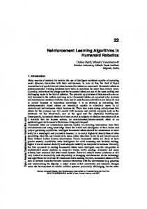
12 Parts of this work appeared in IEEE Transactions on Neural Networks (Vassiliades et al., 2011), in two full conference proceedings/compiled volumes (ICANN 2009, IJCNN 2010) (Vassiliades et al., 2009b; Vassiliades and Christodoulou, 2010b) and several abstracts (Vassiliades et al., 2009a; Vassiliades and Christodoulou, 2010a; Vassiliades et al., 2012). Methodologies similar to this work have been used for modeling the Cyprus problem and are currently at the final preparation for submission (Karaolis et al., 2015). Figure 2.1 illustrates an overview of this chapter. This study draws ideas from the fields of Reinforcement Learning and Evolutionary Computation. The environments used are all multiagent. This study shows that we can achieve desired outcomes by evolving the reward function of the agents.

Figure 2.1: Overview of Chapter 2. This study draws ideas from the fields of Reinforcement Learning and Evolutionary Computation. The environments used are all multiagent. This study shows that we can achieve desired outcomes by evolving the reward function of the agents.

2.2

Introduction

Multiagent Reinforcement Learning (MARL) has attracted an influx of scientific work. The main problem of MARL is that the presence of multiple learning agents creates a nonstationary

13 environment. Such an environment is affected by the actions of all agents, thus, for a system to perform well, the agents need to base their decisions on a history of joint past actions and on how they would like to influence future ones. In MARL there could be different kinds of situations which could be modeled using game theory (Fudenberg and Tirole, 1991; Leyton-Brown and Shoham, 2008; Shoham and Leyton-Brown, 2008): fully competitive or adversarial (which could be modeled with zero-sum games), fully cooperative or coordinative (which could be modeled with team games), and a mixture of both (which could be modeled with general-sum games). Since different issues arise in each situation, a lot of algorithms were proposed to address them. Some of these algorithms are the following: (i) minimax-Q (Littman, 1994), which extends the classic Q-learning algorithm (Watkins, 1989) for single-agent RL by replacing the “max” operator in the update step of Q-learning with one that calculates each player’s best response, and can be applied to two-player zero-sum games; (ii) Nash-Q (Hu and Wellman, 2003), which is an extension of minimax-Q to general-sum games; (iii) Joint Action Learners (Claus and Boutilier, 1998), which is an approach investigated in cooperative settings in which the agents maintain some beliefs about the strategies of the other agents and therefore learn joint action values; (iv) FoF-Q (Friend-or-Foe Q) (Littman, 2001), which can be interpreted as consisting of two algorithms, Friend-Q, which is suited for coordination games and Foe-Q for zero-sum games and is equivalent to minimax-Q; (v) WoLF-PHC (Win or Learn Fast - Policy Hill Climbing) (Bowling and Veloso, 2001), which uses an extension of Q-learning (Watkins, 1989) to play mixed strategies based on the WoLF principle that uses a higher learning rate when the agent is losing and a lower one when it is winning; (vi) WoLF-IGA (WoLF - Infinitesimal Gradient Ascent) (Bowling and Veloso, 2002; Banerjee and Peng, 2002), which combines gradient ascent with an infinitesimal step size (IGA) (Singh et al., 2000) with the WoLF method; (vii) CE-Q (Correlated Equilibria Q) (Greenwald and Hall, 2003), which learns correlated equilibrium (Aumann, 1974) policies and

14 can be thought of as a generalization of Nash-Q and FoF-Q; (viii) FMQ (Frequency Maximum Q) (Kapetanakis and Kudenko, 2005), which is a heuristic method proposed for coordination in heterogeneous environments and is based on the frequency with which actions yielded the maximum corresponding rewards in the past; (ix) GIGA-WoLF (Generalised IGA - WoLF) (Bowling, 2005), which achieves convergence and no-regret (i.e., the algorithm performs as good as the best static strategy); (x) AWESOME (Adapt When Everybody is Stationary Otherwise Move to Equilibrium) (Conitzer and Sandholm, 2007), which is an algorithm that is guaranteed to converge to a Nashequilibrium (Nash, 1950) in self-play and learns to play optimally against stationary opponents in games with an arbitrary number of players and actions; (xi) WPL (Weighted Policy Learning) (Abdallah and Lesser, 2008), which assumes that an agent neither knows the underlying game nor observes other agents, and achieves convergence in benchmark two-player-two-action games, and (xii) M-Qubed (Max or MiniMax Q) (Crandall and Goodrich, 2011), which is a robust algorithm that was shown to achieve high degrees of coordination and cooperation in several two-player repeated general-sum games in homogeneous and heterogeneous settings. For a comprehensive coverage of MARL algorithms, see Bus¸oniu et al. (2008) and references therein. A lot of work is focused in deriving theoretical guarantees, based on different sorts of criteria such as rationality and convergence (Bowling and Veloso, 2001), targeted-optimality, safety and auto-compatibility (Powers et al., 2007) or security, coordination and cooperation against a wide-range of agents (Crandall and Goodrich, 2011). Theoretical work has also been done in analyzing the dynamics of multiagent learning. For instance, Tuyls et al. (2006) investigated MARL from an evolutionary dynamical perspective, while Iwata et al. (2006) approached the field from a statistical and an information theoretical perspective. Since the problem is not very well-defined, Shoham et al. (2007) attempted to classify the existing work by identifying five distinct research agendas. They argued that when researchers design algorithms, they need to place their work

15 under one of these categories which are: (i) computational, which is aimed in designing learning algorithms that iteratively compute properties of games, (ii) descriptive, which is to determine how natural agents (such as humans, animals or populations) learn in the context of other learners and make decisions, (iii) normative, in which the learning algorithms give a means to determine which sets of learning rules are in equilibrium with one another, (iv) prescriptive cooperative, which is how to design learning algorithms in order to achieve distributed control and (v) prescriptive noncooperative, which is how to design effective algorithms, or how agents should act to obtain high rewards, for a given environment, i.e., in the presence of other (intelligent) agents. Subsequently some work did focus on specific agendas (for example see Erev and Roth, 2007), but more agendas were proposed (Gordon, 2007). In addition, the original agendas (Shoham et al., 2007) have been criticized that they may not be distinct, since they may complement each other (Fudenberg and Levine, 2007; Tuyls and Parsons, 2007). Stone (2007) extended the criticism by arguing that the game theoretic approach is not appropriate in complex multiagent problems. Despite these criticisms, our study lies in the original prescriptive non-cooperative agenda (Shoham et al., 2007), i.e., we are interested in effective techniques that result in high rewards for the agents. More specifically, the current study investigates cooperation between self-interested agents in a non-cooperative setting. This situation can be modeled with the Iterated Prisoner’s Dilemma (IPD) which is a general-sum game. It is very interesting and beneficial to understand how and when cooperation is achieved in the IPD’s competitive and contradictive environment, as it could then become possible to prescribe optimality in real life interactions through cooperation, analogous to the IPD. In its standard one-shot version, the Prisoner’s Dilemma (PD) (Rappoport and Chammah, 1965) is a game summarized by the payoff matrix of Table 2.1. There are two players, Row and Column. Each player has the choice of either to “Cooperate” (C) or “Defect” (D). For each pair of choices, the payoffs are displayed in the respective cell of the payoff matrix of Table 2.1. These

16 Table 2.1: Payoff matrix of the Prisoner’s Dilemma game with the most commonly studied payoff values. Payoff for the Row player is shown first. R is the “reward” for mutual cooperation. P is the “punishment” payoff for mutual defection. T is the “temptation” payoff for unilateral defection and S is the “sucker’s” payoff for unilateral cooperation. The only condition imposed to the payoffs is that they should be ordered such that T > R > P > S.

Row Player

Cooperate (C) Defect (D)

Column Player Cooperate (C) Defect (D) R(= 3), R(= 3) S(= 0), T (= 5) T (= 5), S(= 0) P (= 1), P (= 1)

values were used in various IPD tournaments (see for example Axelrod, 1984; Kendall et al., 2007) and to the best of our knowledge are the ones most commonly studied. An outcome is composed from the actions of the two players. For example, the outcome CD means that the Row player selected C (and received the payoff S = 0) and the Column player selected D (and received the payoff T = 5). In game theoretical terms, where rational players are assumed, DD is the only Nash equilibrium outcome (Nash, 1950), (i.e., a state in which no player can benefit by changing his/her strategy while the other players keep theirs unchanged), whereas the cooperative (CC) outcome satisfies Pareto optimality (Pareto, 1906) (i.e., a state in which it is impossible to increase the gains of one player without increasing the losses of other players). The “dilemma” faced by the players in any valid payoff structure is that, whatever the other player does, each one of them is better off by defecting than cooperating. The outcome obtained when both players defect, however, is worse for each one of them than the outcome they would have obtained if both had cooperated. In the IPD, an extra rule (2R > T + S) guarantees that the players are not collectively better off by having each player alternate between C and D, thus keeping the CC outcome Pareto optimal. Moreover, contrary to the one-shot game, CC can be a Nash equilibrium in the infinite version of the IPD (Leyton-Brown and Shoham, 2008).

17 Although the cooperative outcome is a valid equilibrium of the IPD, our study does not aim to assess the strength of the learning algorithms to attain equilibria of the game or best responses to any given strategy. Instead, our goal is to achieve and maintain CC by simple reinforcement learning (RL) agents, as this outcome results in larger cumulative payoffs for both of them. Our preliminary experiments revealed that when two Q-learning or SARSA agents play the IPD, they do not engage in mutual cooperation quickly or consistently and as a result they do not converge to this beneficial outcome. An interesting and revealing observation was that the percentages of the outcomes of the game (such as CC or DD) could dramatically vary when the parameters of the learning algorithms remained the same but the payoff values were changed (within the rules of the game). For this reason we ask whether we can enhance CC by evolving the payoff matrix. The rationale behind this is that we would like to motivate the agents into cooperation by making them perceive the payoff values differently, i.e., as rewards and penalties. The use of an evolutionary algorithm is motivated both by how biological evolution hard-wires primary rewards in animals and by the fact that such algorithms can solve hard problems that have multiple local minima. In this study, we seek to evolve some reward function (shared by both agents) that directly maps the external payoffs into appropriate reinforcement signals that are generated inside the agent. Thus, the evolved payoff values could be thought of representing internal rewards rather than external/environmental stimuli. The mapping between external payoffs and internal rewards is one-to-one for simplicity. As pointed out by Zinkevich et al. (2007) “perfectly predicting the environment is not enough to guarantee good performance”, because the performance depends partly on properties of the environment. In our case, we believe that the property of the environment which plays a significant role in the CC outcome is the reward function (i.e., the payoff matrix), since it specifies the type and strength of the reinforcement the agents receive. Therefore, we introduce a method

18 that evolves the payoff values of the IPD while satisfying its constraints, in order for simple RL algorithms to rapidly reach the CC outcome. The remainder of this chapter is organized as follows. In Section 2.3, we present some related work. Section 2.4 describes our methodology, while the results are given in Section 2.5. Finally, in Section 2.6, we briefly discuss some issues related to this work and summarize our conclusions.

2.3

Related Work

Sandholm and Crites (1996) investigated MARL in the IPD by representing the state-action estimates (Q-function) inside lookup tables and simple recurrent neural networks and showed that lookup tables lead to better results. However, the payoff values they used were a scaled down version of the commonly studied values T = 5, R = 3, P = 1, S = 0. They report results where CC occurred 50% of the time in the final rounds of the game, after running the simulation for 62.5 million rounds. Our previous work with MARL in the IPD (Vassiliades et al., 2009b, 2011), showed that it is possible to train spiking neural networks to reach mutual cooperation. In this case however, a mixture of both positive and negative payoff values is necessary, as the learning algorithms used (Seung, 2003; Florian, 2007), work with positive and negative reinforcements extracted from the payoff matrix and directly applied to the synapses. This mixture was found to be beneficial for non-spiking neural networks as well as lookup tables (Vassiliades et al., 2009b). Reward shaping1 is a technique that introduces supplemental rewards to a reinforcementlearning algorithm, during the learning process, with the purpose of helping the agent learn a desirable behavior more efficiently (see for example Ng et al., 1999; Randløv, 2000). Buffet et al. (2007) proposed a shaping methodology for automatically designing multiagent systems. Their approach was based on progressively growing: (i) the complexity of the task, so that agents would 1

The ‘shaping’ technique goes back to the work of Skinner (1953) (as explicitly stated by Peterson, 2004).

19 incrementally learn harder and harder tasks, and (ii) the multiagent system, by cloning agents that were trained in a simple environment to a more complex one. They tested their approach on simulated environments where the agents had to coordinate in order to reach a common goal and showed that incremental learning results in more efficient learning of complex tasks. Babes et al. (2008) presented a technique they called “social reward shaping” that initializes the Q-function of a Q-learning agent (Watkins, 1989) with values derived from an analysis of a mutually beneficial subgame perfect equilibrium of the IPD. By doing so, they effectively encouraged the agents to converge more quickly to mutual cooperation; this was achieved because the initialization of the Q-function has been shown to be equivalent to adding shaping rewards during the learning process (Wiewiora, 2003). Agents that rely only on pre-designed reward functions in order to be trained might not truly be called adaptive and autonomous, because they can only cope with environment types to which these functions apply. Different approaches addressing this issue do exist (e.g., Ackley and Littman, 1991; Singh et al., 2005). Snel and Hayes (2008) investigated the evolution of valence systems (i.e., systems that evaluate positive and negative nature of events) in an environment largely based on the artificial life world by Ackley and Littman (1991). They compared the performance of motivational systems that are based on internal drive levels versus systems that are based purely on external sensory input and showed that the performance of the former is significantly better than the performance of the latter. Moreover, an elaborated view of the agent-environment interaction (Singh et al., 2005, 2010) splits the environment into the external environment and an internal one, the latter of which is considered to be part of the agent. The external environment provides the sensations to the agent and receives its actions, while the internal environment provides the states and rewards to the agent (since it contains the critic), and receives the agent’s decisions. Such intrinsic rewards can be used

20 to implement curiosity-driven agents (Schmidhuber, 1991). Some other line of work shows that by discriminating external rewards from “utilities” (i.e., internal stimuli elicited by rewards) and using utilities for learning in the IPD, cooperation can be facilitated (Moriyama, 2009). Singh et al. (2009) introduced a framework for reward that complements existing RL theory by placing it in an evolutionary context. They demonstrated the emergence of reward functions which capture regularities across environments, as well as the emergence of reward function properties that do not directly reflect the fitness function. In the case of the IPD, there have been some studies that examined the impact of varying the payoff values. Johnson et al. (2002) investigated the reason why the PD has hardly been found in nature. They argued that the assumption of a fixed payoff matrix for each player is not realistic due to variations between individuals on the payoff matrix. They examined the effect of: (i) adding normally distributed random errors to the payoff values, and (ii) the spacing between payoffs. They showed that frequent violations of the payoff structure occur when the interval between payoffs is low. Chong and Yao (2006) introduced a co-evolutionary framework where each strategy has its own self-adaptive payoff matrix. The adaptation of each payoff matrix is done by an update rule that provides a form of reinforcement feedback between strategy behaviors and payoff values. By relaxing the restriction of a fixed and symmetric payoff matrix, they showed how different update rules affected the payoff values and subsequently the levels of cooperation in the population. Rezaei and Kirley (2009) investigated cooperation in a spatial version of the PD game. They provided each agent with its own payoff matrix which was affected by attributes such as the agent’s age and experience level. They showed that time-varying non-symmetric payoff values promote cooperation in this version of the game.

21 2.4

Methodology

As we mentioned in Section 2.2, the purpose of this work is to evolve the payoff values of the IPD (i.e., T , R, P , S), in order to find more appropriate rewards for the agents, which would motivate them to cooperate. A preliminary investigation was performed with the popular payoff values T = 5, R = 3, P = 1 and S = 0, and 2 Q-learning agents using -greedy exploration (where a random action is chosen with probability , otherwise the greedy action is chosen (Sutton and Barto, 1998)) with = 0.1, while the game simulation ran for 30 independent trials, each lasting 60000 rounds. The results showed that the agents do not engage in mutual cooperation. The following sections describe our methodology, which is split into two phases: the first is the evolutionary simulation, where the payoffs are optimized, and the second is the evaluation phase.

2.4.1

Evolution phase

For the evolution phase we describe below the MARL simulation that takes place during each fitness evaluation, a method that generates an initial population of valid solutions for the IPD, two mutation operators that alter the individuals but do not change their validity, and the evolutionary algorithm used.

2.4.1.1

Multiagent Reinforcement Learning Simulation

The environment is set to be the IPD and the agents implement the Q-learning algorithm (Watkins, 1989). The step size parameter, α, as well as the discount factor, γ, are empirically set to 0.9. We use lookup tables to represent the value function and not function approximators, such as neural networks, as previous work showed that lookup tables yield better results in these settings (Sandholm and Crites, 1996; Vassiliades et al., 2009b). This is because the state-action space is simple, so there is no need to generalize from previously experienced states to unseen

22 ones. In addition, lookup tables are provably convergent with Q-learning (under certain conditions), whereas function approximators may diverge (see, for example, Boyan and Moore, 1995; Baird, 1995; Baird and Moore, 1999; Wiering, 2004). At every round each agent chooses either to Cooperate (C) or Defect (D), and is provided with incomplete information. In particular, each agent receives only the state of the environment, i.e., the actions of both itself and its opponent in the previous round, as well as the payoff associated with its action, but not the payoff associated with the opponent’s action. Both agents need to learn a policy that maximizes their long-term rewards and the only way to achieve that is by learning to cooperate. A Boltzmann exploration schedule is utilized, as it gives a good balance between exploration and exploitation, as well as fast convergence. More specifically, an action ai is selected in state s with probability p(ai ) given by Equation 2.1: p(ai ) =

eQ(s,ai )/t X eQ(s,a)/t

(2.1)

a∈{C,D}

where Q(s, ai ) is the value of choosing action ai in state s and the temperature t is given by t = 1 + 10 × 0.99n , with n being the number of games played so far. The constants 1, 10 and 0.99 are chosen empirically. More specifically, 10 and 0.99 are chosen because we want to move from exploration to exploitation in less than 1000 rounds, while the constant 1 is added to restrict the temperature from falling below that value. The latter was done in order to preserve some stochasticity in action-selection, unless the difference in Q values (of the actions from a certain state) is significant, in which case the policy will be nearly identical to the greedy policy; this will in turn force evolution to find a more appropriate reward function. The number of rounds is set to 1000 and the percentages of all outcomes (CC, CD, DC, DD) are averaged over 30 trials in order to get a smoother estimate of the fitness.

23 2.4.1.2

Generating Valid Solutions for the IPD

When generating the initial population, we need to ensure that all individuals consist of payoff values that fall inside the rules of the game. If not, then we need to assign a penalty term on the fitness function in order to be fair with all individuals. However, by evolving the payoff values with this approach, the final solutions might still not satisfy the IPD rules. Moreover, it might be difficult to construct a penalty function for this purpose. One way to generate valid individuals is to randomly assign the T , R, P , S values and reject solutions that are invalid or use a repair method to ensure that they will satisfy the rules. Another way is to incrementally construct and repair the values by utilizing domain knowledge (i.e., the rules of the game) at every step. We use the latter approach and more specifically, we randomly generate the values of each individual, all uniformly distributed within the bounds specified below, in the following sequence: 1. T 0 ∈ (bmin , bmax ) 2. S 0 ∈ (bmin , T 0 ) 3. P 0 ∈ (S 0 , T 0 ) 4. R0 ∈ (max(P 0 , (T 0 + S 0 )/2), T 0 ) where the primed payoff values (T 0 , R0 , P 0 , S 0 ) are the newly generated values. The lower bound of R0 is max(P 0 , (T 0 + S 0 )/2) because we know from the rules of the game that R0 should be greater than both P 0 and (T 0 + S 0 )/2, and P 0 could either be less or greater than (T 0 + S 0 )/2. The payoffs need to be generated in this order to ensure that each individual will satisfy the constraints of the game. The initial lower bound, bmin , and initial upper bound, bmax , are the bounds of the values within which the initial population is generated. We also set some absolute lower and upper bounds, Bmin = −50 and Bmax = 50, in order to restrict the search space. The

24 values −50 and 50 are chosen empirically. In Section 2.5, we present some experiments where we vary the bounds [Bmin , Bmax ], but never go beyond [-50,50]. In addition, in some experiments we set the bounds of the initial population [bmin , bmax ) either to [Bmin , Bmax ) (which may change according to the experiment), or [0, 1). When initializing the values of the population in the range [Bmin , Bmax ) we effectively help evolution to converge more quickly, since the individuals span the entire search space and not just one region of it (such as [0, 1)). The reason why we have chosen to sometimes initialize the population to the range [0, 1) is to show that evolution manages to find very good solutions even though the initial population is not spread in the entire search space. We also conducted experiments where all individuals in the population were initialized to the values of Table 2.1 and the results did not display any significant difference from the results obtained using any other initialization we tested, therefore we do not report them for brevity.

2.4.1.3

Mutation Operators

In order to introduce variation into the population, two mutation operators are implemented, OP 1 and OP 2 . OP 1 changes the magnitude and relative distance between the payoffs by selecting uniformly distributed values for each payoff T, R, P and S, within the following bounds: • T 0 ∈ (R, min(2R − S, Bmax )) • R0 ∈ (max(P, (T + S)/2), T ) • P 0 ∈ (S, R) • S 0 ∈ (Bmin , min(P, 2R − T )) These bounds were calculated from the rules of the game. For example, when considering the value T 0 , we know from the rule R > (T + S)/2 that T < 2R − S. Since 2R − S could be

25 less or greater than the upper bound of the search space, Bmax , the upper bound of T 0 should be min(2R − S, Bmax ). In contrast with OP 1 , OP 2 keeps the magnitude and relative distance between the payoffs the same, but it effectively shifts them as follows: a random value is generated from the normal distribution N (0, 1) and added on all the payoff values; if the new payoff values go out of bounds (i.e., S 0 < Bmin or T 0 > Bmax ) this is repeated. It is important to note that if the parent payoff values satisfy the rules of the game, this shifting operator generates a valid offspring solution.

2.4.1.4

Evolving payoff values for the IPD

When deciding which fitness function to use, we need to base our decision on a function that is more informative in terms of our goal, which is the fast convergence to the cooperative outcome (CC). We could design our fitness function to be the accumulated payoff of the system (i.e., the sum of the accumulated payoffs of the two agents), since in the IPD the CC outcome results in the highest payoff of the system. However, if we wanted to compare the performance of the system when using payoff matrices that have only negative values, as opposed to when using payoff matrices that have only positive values, this fitness function becomes problematic. The reason is that when using negative payoff values, the fitness value will be negative, whereas when using positive payoff values, the fitness value will be positive. Therefore we need a fitness function that is independent of the payoff and dependent only on the outcome of the game. Such function is the one we are using where the fitness of an individual fi is calculated as shown in Equation 2.2: fi = CC i − CDi − DC i − DDi

(2.2)

where i is the individual (i.e., payoff matrix) being evaluated, and CC i , CDi , DC i , and DDi are the percentages of the corresponding outcomes at the end of the rounds averaged over all rounds and trials. By trying to maximize this function, we effectively find solutions that maximize the

26 cooperative outcome and minimize all other outcomes. Therefore, a value of 1 means that the game simulation consists of only the CC outcome, a value of 0 means that the CC outcome occurs 50% of the time and a value of -1 means that the CC outcome never occurred in the simulation. A (µ + λ)-truncation selection is used which means: 1. µ is the population size and λ = 2∗µ, i.e., for each parent individual we generate 2 offspring (one from each mutation operator), 2. we rank all individuals (parents µ and offspring λ) based on their fitness and 3. the best µ individuals from parents and offspring are selected as the new parents for the next generation. The number of evolution trials is set to 30, the population size to 10 and evolution is repeated for 50 generations. The pseudo-code is illustrated in Figure 2.1. Algorithm 2.1: Pseudo-code of the evolutionary algorithm. Each mutation operator generates one offspring for each member of the population and the best individuals from both parents and offspring are selected for the next generation. 1 2 3 4 5 6 7 8 9 10 11 12

foreach evolution trial do generate and evaluate initial population (P); foreach generation do foreach Individual i ∈ P do Offspring1[i] = mutationOP1(P[i]); Offspring2[i] = mutationOP2(P[i]); evaluate(Offspring1[i]); evaluate(Offspring2[i]); end P = truncSelection(P, Offspring1, Offspring2); end end

27 2.4.2

Evaluation phase

The second phase of our methodology, i.e., the evaluation phase, occurs after we obtain the results from the evolutionary simulation. In the evaluation phase, we take the evolved reward function, i.e., the evolved payoffs that are found from the evolution phase, and use them instead of the external payoff values. To distinguish the Q-learning agent that uses this reward transformation process, we call it “Reward Transformation Q-learning” (RTQ). In this phase, we use the following external payoff values: T = 5, R = 4, P = −2, and S = −3. These are used to measure the performance of the system. In the evaluation phase we also store the value function in a lookup table, and the agents are provided only with incomplete information: they only receive the state of the environment, i.e., the actions of both the agent and the opponent in the previous round, but not the payoffs associated with their opponent’s action. As in the evolution phase, the same Boltzmann exploration schedule is utilized with the same annealing formula (see Equation 2.1). Two types of simulations were performed: (1) between a learning and a non-learning agent, and (2) between two learning agents.

2.4.2.1

Learning Agents Against Non-Learning Opponents

These initial simulations compare three learning agents against opponents that do not use any learning algorithm (single-agent RL). Our learning agents are the following: (a) “Q” (for Qlearning), (b) “SARSA” and (c) “RTQ” (for Reward Transformation Q-learning), i.e., the agent that transforms the external payoff values to different internal rewards. The rewards given to Q and SARSA are the same as the external payoff values. The non-learning opponents are named after the strategies they use: “OnlyCooperate” selects only the Cooperate (C) action, “OnlyDefect” selects only the Defect (D) action, “Random(p)” selects a random action with a specified

28 probability of cooperation p, “Tit-for-Tat” (TFT, Axelrod and Hamilton, 1981) starts with action C and afterwards repeats its opponent’s previous action, and “Pavlov” (also known as “Win-Stay, Lose-Shift”, Nowak and Sigmund, 1993) changes its actions only if the two lowest payoffs, S and P, were received.

2.4.2.2

Learning Agents Against Learning Opponents

The latter simulations compare two learning agents (i.e. Q, SARSA and RTQ) against each other (i.e., we have a MARL setting). The multiagent system can either be homogeneous or heterogeneous where: (i) a homogeneous system is when both agents employ the same learning algorithm, with the same or similar parameters and (ii) a heterogeneous system is when both agents employ the same algorithm with dissimilar parameters, or different algorithms. The parameters are the step size, α, and the discount factor, γ.

2.5

Results and Discussion

2.5.1 2.5.1.1

Evolution phase Evolution of payoffs

In this first experiment we evolve the payoffs in the range Bmin = −50 and Bmax = 50. The bounds of the values of the initial population are set to bmin = 0 and bmax = 1. Figure 2.2 illustrates how the probability of mutual cooperation (CC) between the agents changes with the game rounds, when using the initial payoff values and the payoff values found by evolution. The evolved values are the following: T = 6.37, R = 3.01, P = −41.04 and S = −44.05. It is clear that the probability of CC when the evolved values are used becomes almost equal to 1 at the end of the simulation, which means that the agents start cooperating from very early in the game.

29 Note that if the number of rounds is increased even further, then this measure of the probability of CC will converge to some asymptotic value; it will never reach the value of one as it is essentially calculated as the percentage of CC over all previous rounds (averaged over multiple trials) up to the current round in the simulation. It is interesting to observe that while P and S become close to Bmin , T and R do not become close to Bmax . This may suggest that when “winning”, the agents should accumulate small amounts of reward, whereas when “losing”, the agents need to lose much, in order to understand that such behavior is detrimental. 1

Probability of CC

0.8 Initial Values

0.6

Evolved Values 0.4 0.2 0

0

200

400 600 Rounds Played

800

1,000

Figure 2.2: Probability of mutual cooperation (CC) over time when the Q-agents learn using the initial payoff values (dotted line) and the evolved payoff values (solid line). The evolved values make the agents reach mutual cooperation very early in the game, whereas with the initial values the agents do not learn to cooperate in 1000 rounds, as the probability of CC reaches only 0.12.

2.5.1.2

Effect of the lower/upper bounds

In the second experiment we investigate how the absolute lower and upper bounds (i.e., parameters Bmin and Bmax ) affect the solutions, with the purpose being to check whether the magnitude of rewards is important. More specifically, we check 6 cases for the range [Bmin , Bmax ]: [−1, +1], [−2, +2], [−4, +4], [−8, +8], [−16, +16] and [−32, +32]. The range of the values of the initial population [bmin , bmax ) is set to [0, 1). Table 2.2 shows a comparison between these cases based on the fitness of the best individual found by evolution. It is clear that as the range

30 Table 2.2: Fitness values of the evolved solutions in the bounds specified. As the range of the payoffs increases, so does the fitness (highest fitness shown in bold). The fitness of the payoff values of Table 2.1 is shown for comparison in the first row of the table.

Configuration T = 5, R = 3, P = 1, S = 0 [−1, +1] [−2, +2] [−4, +4] [−8, +8] [−16, +16] [−32, +32]

Fitness -0.769 0.045 0.478 0.557 0.618 0.775 0.910

of the values increases so does the fitness. Therefore, by allowing higher magnitudes of evolved rewards/payoffs the system reaches mutual cooperation more often. If the range of the initial population [bmin , bmax ) is set to [Bmin , Bmax ) in each case, the results are approximately the same; the only difference is that in the latter case, individuals with high fitness are found earlier, since their values span the entire search space instead of just one region (i.e., [0, 1)).

2.5.1.3

Effect of the reward sign

The third experiment deals with the sign of the rewards. The bounds of the payoffs are kept in a range equal to 5, which is the range specified by the values of the initial case (T = 5, R = 3, P = 1, S = 0). More specifically, we check whether evolved solutions that contain all positive values, all negative values, or a mixture of both positive and negative values give better results than the initial case. We test 8 configurations by varying the bounds [Bmin , Bmax ] from [−6, −1] to [1, 6] incrementing them by 1 in every configuration. The range of the values of the initial population [bmin , bmax ) is set to [Bmin , Bmax ) in each configuration. Table 2.3 compares these configurations based on the average fitness of the best individual found by evolution.

31 We observe that when the values of the bounds are negative, the fitness values are greater than 0.5 which means that mutual cooperation occurred more than 75% of the time. The fitness values rise slightly further with the introduction of small positive values; however, as the “penalty” (i.e., negative values) is reduced by moving towards bounds with only positive values, the percentage of mutual cooperation decreases. The highest fitness and thus percentage of mutual cooperation is observed for the range [−3, 2] (as shown in bold). Table 2.3: Fitness values of the evolved solutions in the bounds specified. Highest fitness is observed for the range [−3, 2] (shown in bold). The fitness of the payoff values of Table 2.1 is shown for comparison in the first row of the table.

Configuration T = 5, R = 3, P = 1, S = 0 [−6, −1] [−5, 0] [−4, +1] [−3, +2] [−2, +3] [−1, +4] [0, +5] [+1, +6]

Fitness -0.769 0.523 0.525 0.547 0.548 0.492 0.437 0.326 0.187

It is worth noting that for the range [0, +5], in contrast with the payoff values of Table 2.1 which have the same range, the evolved payoffs have a positive fitness. The reason why this happens is illustrated more clearly in Figure 2.3. The values of the evolved matrices from all configurations appear to follow a pattern. The P and S values become close together and closer to the lower bound, while the values T and R become close together, but closer to the upper bound especially when the values of the bounds are negative. As the values of the bounds increase, T and R seem to be moving away from the upper bound.

Payoff values

32 6 5 4 3 2 1 0 -1 -2 -3 -4 -5 -6

R S T P

[-6,-1]

[-5,0]

[-4,1]

[-3,2]

[-2,3]

[-1,4]

[0,5]

[1,6]

Bounds of the payoff values

Figure 2.3: Evolved payoffs for every range configuration. Boxes indicate the bounds of the corresponding configuration. The following pattern is observed: the values P and S become close to the lower bound of the range specified, while the values T and R become close to the upper bound when the range “includes more” negative values, and seem to be moving away from the upper bound when the range “includes more” positive values. 2.5.1.4

Effect of the population size

In this experiment, the effect of the population size (p) on the quality of solutions is examined. In particular, population sizes of 1, 2, 4, 6, 8, 10 and 12 are investigated. The bounds of the search space Bmin and Bmax are set to -50 and 50 respectively, as described above, and the range of the initial population, [bmin , bmax ), is set to [0,1). The results are depicted in Figure 2.4, where for each population size, the bars show the evolved payoff values, while the corresponding fitness value is written next to them. We observe that as the population size increases, evolution finds better solutions; however, for p = 10 and p = 12 the fitness is approximately the same suggesting that there is no significant improvement with population sizes above 10. Good solutions are found even when there is only 1 individual in the population. This shows that the problem of evolving the payoff values is solved easily. We observe that in fitter solutions, the values T and R are closer together, while the P and S values are closer together and closer to the lower bound. This is better illustrated when comparing the solution found when p = 1, with the solution found when p = 12. It is interesting to note

Population Size

33

12

0.957

10

0.957

8

0.954

6

0.951

4

0.936

2

0.894

1

0.847 -50

-40

-30

-20

-10

0

10

T R P S

20

30

Payoff Values

Figure 2.4: Evolved payoff values with their fitness (written next to the bars) for different population sizes. Larger population sizes result in better solutions, while good solutions are also found with small population sizes. There is no significant improvement in the fitness with population sizes above 10. While the values P and S are closer to the lower bound, the values T and R are less than 10. 1

Fitness

0.8 0.6 0.4 0.2 0

p = 1 p = 2 p = 4 p = 6 p = 8 p = 10 p = 12

0

10

20 30 Generation

40

50

Figure 2.5: Fitness values of the best solution found for different population sizes (p) over the generations. Good solutions are obtained in less than 10 generations for all populations. that for all population sizes, while the values P and S are closer to the lower bound, the values T and R are less than 10. The effect of the population size is also depicted in Figure 2.5, where the fitness of the best individual for different population sizes, is shown over the generations.

34 2.5.1.5

Effect of the mutation operators

Finally, we examine the role of the mutation operators throughout the evolutionary process and how they affect the solutions. In order to do so, we mark each offspring, whenever it is generated, by a value that indicates which mutation operator created it (OP1 or OP2). After ranking the population in order to select the best elite individuals, we count how many individuals were generated by each mutation operator. At the beginning of each generation, this mark is reset for every member of the population. These counters are averaged over 30 evolution trials, as in all other results. Figure 2.6 shows the average number of mutated solutions over the generations with each mutation operator. We notice that OP1 is mostly used in the beginning, thus, we could say that it mostly contributes to the exploration of the search space, while OP2 is used both in the beginning and afterwards, thus explores and fine-tunes the solutions. Towards the end of evolution, the average number of mutated individuals is less than 1, since all members of the population have converged and the quality of solutions cannot be improved any further. It is worth noting that these results are consistent with all population sizes. Number of mutated individuals

5 4 OP1

3

OP2 2 1 0

0

10

20 30 Generation

40

50

Figure 2.6: Average number of mutated individuals over the generations with each mutation operator (OP1 and OP2). OP1 (solid line) is activated more in the beginning of evolution, therefore it mostly contributes to the exploration of the search space, while OP2 (dotted line) is activated both in the beginning and afterwards, thus explores and fine-tunes the solutions. Towards the end of evolution, the average number of mutated individuals is less than 1, since all members of the population have converged and the quality of solutions cannot be improved any further.

35 2.5.1.6

Strategies emerged

By examining the final action-value (Q) functions of the agents after learning, using the evolved payoff values of the best individual from the last generation, we can determine what kind of reactive (i.e., memoryless) deterministic policies emerged in each evolutionary run. That is, if after learning, the agents switch off exploration, and greedily select the action that has the best action-value estimate in each state (CC, CD, DC, DD), we can determine the strategies that emerge from evolution and learning. There are 24 = 16 possible strategies, due to the fact that there are 2 actions and 4 states. Out of these, two are of particular interest: the TFT strategy and the Pavlov (i.e., “Win-Stay, Lose-Shift”) strategy. We tested the evolved payoff values of each evolutionary run for one RL simulation (compared to 30, as was done during evolution) and observed the following: in 14 cases the final strategy of both agents was the Pavlov, in 9 cases the final strategy of both agents was the TFT, whereas in the remaining 7 cases the final strategies were different for each agent. For example, in one of these cases, the final strategy of the first agent was the Pavlov, whereas the strategy of the second agent was the TFT. In another case, the strategy of one of the agents resembled a mixture of Pavlov and TFT, i.e., from CC it chooses C (as in both TFT and Pavlov), from CD it chooses D (as in both TFT and Pavlov), from DC it chooses C (as in TFT), and from DD it chooses C (as in Pavlov).

2.5.2

Evaluation phase

The games are run for 50 trials with 1000 rounds per trial. All combinations of agents are tested with α and γ taking the values 0.1 or 0.9 (i.e., slow/fast learning, weak/strong discounting). For the RTQ agent we use the following internal reward values, which were found from the experiments of the previous section to provide a high amount of mutual cooperation: T 0 = 3.81, R0 = 1.76, P 0 = −44.82 and S 0 = −46.32.

36 2.5.2.1

Learning Agents Against Non-Learning Opponents

As described in Section 2.4.2, the first simulations are between 3 learning agents (i.e., Q, SARSA and RTQ) and opponents that do not use any learning algorithms (i.e., OnlyCooperate, OnlyDefect, Random, TFT and Pavlov). Table 2.4: Results with learning agents against non-learning opponents. The highest ranking performance for each learning agent is shown in bold (see text for explanation of the basis of the rankings). Highest CC is achieved when an RTQ agent competes against a Tit-for-Tat or a Pavlov opponent. Learning Agent α γ RTQ 0.1 0.9 SARSA 0.1 0.9 Q 0.1 0.9 RTQ 0.9 0.1 SARSA 0.9 0.9 Q 0.9 0.1 RTQ 0.9 0.9 SARSA 0.9 0.9 Q 0.9 0.9 RTQ 0.9 0.9 SARSA 0.9 0.9 Q 0.9 0.9 SARSA 0.9 0.9 Q 0.9 0.9 RTQ 0.9 0.1 Q 0.1 0.9 SARSA 0.1 0.9 RTQ 0.9 0.1 Q 0.1 0.9 SARSA 0.1 0.9 RTQ 0.9 0.1

Non-Learning Agent OnlyCooperate

OnlyDefect

TitForTat

Pavlov

Random(p = 0.25)

Random(p = 0.50)

Random(p = 0.75)

CC 6 15 20 0 0 0 99 95 93 99 93 91 5 6 6 8 8 14 14 14 26

Outcome (%) CD DC DD 0 94 0 0 85 0 0 80 0 25 0 75 25 0 75 32 0 68 0.5 0.5 0 2 2 1 3 3 1 0 0.5 0.5 1 3 3 1 4 4 14 20 61 19 19 56 20 18 56 8 42 42 9 42 41 13 37 36 4 62 20 5 61 20 9 49 16

Table 2.4 shows the best results of the simulations between the 3 agents and the non-learning opponents. In terms of performance, they are ranked based on the percentage of: (a) DC in the case of OnlyCooperate opponent, since the agent needs to learn to play D in order to exploit its opponent’s weakness and accumulate more reward, (b) DD in the case of OnlyDefect, as the agent

37 needs to learn to play D so that it does not get exploited by the opponent, (c) CC in the cases of TFT and Pavlov, since CC can be attained against such reactive opponents, (d) DD in the case of Random(p = 0.25), since this agent is similar to the OnlyDefect agent with the difference being that it cooperates with a small probability, (e) DC and DD in the case of Random(p = 0.50), as this agent cooperates half of the time, and (f) DC in the case of Random(p = 0.75), since this agent is similar to the OnlyCooperate agent with the difference that it defects with a small probability. The results show that the RTQ agent achieves the DC outcome faster than SARSA and Q, when playing against OnlyCooperate, which is most probably due to the fact that the rewards it uses (T 0 and R0 ) are smaller than the corresponding payoff values. The difference between SARSA and Q is negligible. When playing against OnlyDefect, RTQ and SARSA achieve 75% DD and Q only 68%. As this is a simple deterministic bandit problem (where the agents are facing the problem of selecting C or D and receiving the rewards S or P ) we would have expected the agents to play D more. The results shown in Table 2.4 were obtained with the exploration method described in Section 2.4.2, which was chosen to illustrate rapid convergence to the CC outcome in the MARL case and more specifically, for RTQ in self-play, as shown in Section 2.5.2.2. Simulations with greedy exploration (with = 0.1) (not shown) demonstrated that against the OnlyDefect opponent, all 3 agents reach the DD outcome nearly 95% of the time with α = 0.9 and γ = 0.1, for the same number of trials and rounds; the remaining 5% can be attributed to exploration. When the opponent was a TFT agent, RTQ achieves CC 99% of the time, followed by SARSA and then Q, where CC attained 95% and 93% respectively. Similar results are observed when the opponent is Pavlov, where RTQ manages to achieve CC 99% of the time, but SARSA 93% and Q 91%. It is worth noting that for both TFT and Pavlov when the discount factor of the learning agents was low (i.e., γ = 0.1), CC percentage was 70 − 76% for RTQ and 18 − 25% for both Q and SARSA (results not shown). This indicates that a high discount factor is required to reach and maintain

38 mutual cooperation. Against the Random(p = 0.25) opponent (i.e., the agent that chooses C with probability 0.25), SARSA achieves DD 61% of the time, while Q and RTQ 56%. As with the case of the OnlyDefect opponent, results with -greedy exploration (with = 0.1) (not shown) indicate that the learning agents play D more often than in the case of softmax exploration, since the DD outcome occurs 69% of the time with Q and SARSA and 67% of the time with RTQ (α = 0.9 and γ = 0.1 for all agents, and the number of trials and rounds was kept the same as in all simulations). As the Random agent becomes more cooperative (p = 0.50, p = 0.75) the DD outcome diminishes, while the DC outcome rises, for all learning agents.

2.5.2.2

Learning Agents Against Learning Opponents

In the previous section the problem was effectively single-agent RL, as the opponents did not use any learning algorithms. This section deals with the MARL problem. More specifically, the 3 learning agents play against each other and themselves under different parameter settings. Figure 2.7 depicts the results of the RTQ agent against itself, ranked by the percentage of CC. The system is homogeneous (i.e., both agents use the same parameters) only in the 5th, 7th, 8th and 10th cases. Interestingly, the results illustrate that CC is highest (i.e., 97% in the 10th case) when both agents learn fast (α = 0.9) and use weak discounting (γ = 0.1). It has to be noted that at the 200th round the percentage of CC was already very high, i.e., 89% and the accumulated reward of the system, i.e., the sum of rewards of the agents was 1401.52, while the theoretical maximum that corresponds to playing CC all the time (thus receiving R + R = 4 + 4 = 8 for each round) is 1600 (200 × 8). Although not shown here, convergence to the CC outcome was observed only for the best four cases (cases 7-10 of Figure 2.7), and was measured with two metrics. More specifically, for every round we calculate: (a) the deviation of the reward the system receives (i.e., the sum of the agents’

39

1) RTQ (α =0.9, γ =0.9) vs RTQ (α =0.1, γ =0.9)

8

64

2) RTQ (α =0.9, γ =0.9) vs RTQ (α =0.1, γ =0.1)

75

3) RTQ (α =0.9, γ =0.1) vs RTQ (α =0.1, γ =0.9)

75

4) RTQ (α =0.1, γ =0.9) vs RTQ (α =0.1, γ =0.1)

15

8

7

4

86

7) RTQ (α =0.1, γ =0.1) vs RTQ (α =0.1, γ =0.1)

12 9 5

6

4 4

6

3 3 5

89

8) RTQ (α =0.9, γ =0.9) vs RTQ (α =0.9, γ =0.9)

5 5

84

6) RTQ (α =0.9, γ =0.1) vs RTQ (α =0.1, γ =0.1)

10

9 6

80

5) RTQ (α =0.1, γ =0.9) vs RTQ (α =0.1, γ =0.9)

13

21 3

94

9) RTQ (α =0.9, γ =0.9) vs RTQ (α =0.9, γ =0.1)

96

211

10) RTQ (α =0.9, γ =0.1) vs RTQ (α =0.9, γ =0.1)

97

111

CC

CD

DC

DD

0%

10%

20%

30%

40%

50%

60%

70%

80%

90%

100%

Figure 2.7: Performance of Reward Transformation Q-learning (RTQ) agent against itself with different parameter settings ranked according to the percentage of mutual cooperation (CC). Highest CC is achieved when both agents learn fast (α = 0.9) and have weak discounting (γ = 0.1). rewards) from the “desired” one that corresponds to the CC behavior (and is equal to 8 according to the external payoff values given; see Section 2.4.2), and (b) the rate of change of the Q values, whose calculation involves normalization to accommodate for the fact that the scale of rewards of the RTQ agent is different from the one of the Q and SARSA agents. Slower learning, by at least one of the agents, seems to decrease the percentage of the CC outcome because the agents might need more time to converge. This is clearly illustrated in Figure 2.7, since the best three results (cases 8-10) are obtained when both agents learn fast. The only exception is observed between the 6th and 7th cases: when both agents use smaller learning rates and discount factors, the performance of the system is better (i.e., 89% in the 7th case) than when the first agent switches to a higher learning rate (i.e., 86% in the 6th case). This might suggest that the system should be homogeneous (as in the 7th case).

40 On the other hand, weak discounting, at least by one of the agents, seems to increase performance, as the CC outcome occurs more frequently. For example, consider the 1st and 2nd cases: the first agent uses a high learning rate and discount factor, whereas the second agent uses low ones (2nd case); when the second agent switches to a large discount factor (1st case) the CC performance drops from 75% to 64%. This is more clearly illustrated in the 8th, 9th and 10th cases (i.e., the best 3 configurations): starting from a high discount factor for both agents, the performance increases as one agent switches to a low discount factor (i.e., from 94% to 96%) and increases even more as the other agent switches to a low discount factor as well (97%). It is worth noting that this observation is in contrast with the results obtained when all learning agents competed against the reactive opponents TFT and Pavlov in Section 2.5.2.1, as a higher discount factor is required there in order to reach the CC outcome. The exception is found between the 4th and 5th cases: both agents use a smaller learning rate and the first agent uses a high discount factor, whereas the second agent uses a low one (4th case); when the second agent changes to a high discount factor, the performance increases from 80% to 84% (from 4th to 5th case). This might suggest that the system should be homogeneous (as in the 5th case). Figure 2.8 shows the best results from the comparison of the other learning agents, ranked based on the CC percentage. Here the system is homogeneous in the 1st, 3rd, 8th and 10th cases. Comparing the 1st and 10th cases, when both Q-agents switch from a high discount factor (1st case) to a low one (10th case), CC occurs more frequently, i.e., from 41% to 69% of the time. Similar results are obtained with SARSA agents (3rd and 8th cases), where the CC percentage changed from 48% to 66%. The configurations “Q vs SARSA” (2nd and 9th cases) have similar results as well, since the performance changed from 43% to 68%. When RTQ competes with SARSA the results follow the same pattern (i.e., highest CC percentage when both agents are myopic); this does not happen however when RTQ competes with Q. More specifically, when

41

1) Q (α =0.9, γ =0.9) vs Q (α=0.9, γ =0.9)

41

2) Q (α =0.9, γ=0.9) vs SARSA (α=0.9, γ =0.9)

43

3) SARSA (α =0.9, γ=0.9) vs SARSA (α=0.9, γ =0.9)

13 14

48 50

5) RTQ (α =0.9, γ =0.1) vs Q (α=0.9, γ =0.1)

52

59

68

10) Q (α =0.9, γ =0.1) vs Q (α=0.9, γ =0.1)

69

DD

0%

10%

20%

9

25 29

11

26

15

9) Q (α =0.9, γ=0.1) vs SARSA (α=0.9, γ =0.1)

DC

29

11 9

66

CD

11

8

8) SARSA (α =0.9, γ=0.1) vs SARSA (α=0.9, γ =0.1)

CC

31

16

54

7) RTQ (α =0.9, γ =0.9) vs Q (α=0.9, γ =0.9)

31

12 12

4) RTQ (α =0.9, γ=0.9) vs SARSA (α=0.9, γ =0.9)

6) RTQ (α =0.9, γ=0.1) vs SARSA (α=0.9, γ =0.1)

15

30%

7 9

8

8 8 40%

50%

60%

19

70%

17

8 8 80%

16 15 90% 100%

Figure 2.8: Performance of Q-learning, SARSA and Reward Transformation Q-learning (RTQ) agents against each other in homogeneous and heterogeneous configurations ranked based on the percentage of mutual cooperation (CC). Highest CC is achieved for Q-learning with α = 0.9 and γ = 0.1 in self-play. switching from farsighted to myopic agents, in the former case the percentage of CC increases from 50% to 54%, whereas in the latter case CC decreases from 59% to 52%. It is worth noting that none of the configurations converged. Although not shown in Figure 2.8, when the learning rate is low, the DD outcome occurs more frequently. The parameters that were found to increase DD are α = 0.1 and γ = 0.9 for both agents, except for the case of “RTQ vs SARSA”, where both agents used a low discount factor and RTQ used a high learning rate while SARSA a low one. For all these configurations, the range of mutual defection was 41% - 46%, but the systems did not converge. By observing the Q values, we noticed that in the best three configurations of Figure 2.7 (cases 8-10, where two RTQ agents with α = 0.9 competed), at the end of the simulation the Q value corresponding to state CC and action C converged to a positive number, whereas all the other Q values converged to negative numbers, for both agents. In the best three configurations

42

Average Accumulated Payoff

1,600

1,200

800

400

0

0

50

100 Rounds Played

150

200

Figure 2.9: Performance of Q-learning agents: effect of the evolved internal rewards on the accumulated payoff. The performance of the system when both agents use internal reinforcement signals (thick solid line) and when the source of reinforcement is the payoff matrix (dashed line). The performance increased significantly when the internal reinforcement signals were used. The agents managed to engage in mutual cooperation. The theoretically best performance is shown for comparison (dot-dashed line). of Figure 2.8 (cases 8-10) we observed something different: the separation of the Q values to positive, for the ones that correspond to action C from any state, and negative, for the ones that correspond to action D from any state, for both agents; however, a plateau had not been reached. This separation of the Q values was not observed in the worst case of Figure 2.8 (case 1), where the discount factor for both Q-agents was set to 0.9, as some values that were positive for the first agent, were negative for the other agent and vice versa. In order to show the effect the evolved internal rewards have on the performance of the system, in terms of the accumulated payoff over time, we need to compare two configurations that have the same parameters but change only the type of agents from Q to RTQ (since RTQ agents use the Q-learning algorithm with different reinforcement signals). This effect is clearly illustrated in Figure 2.9, where the best configuration (10th case) of Figure 2.7 is compared with the best configuration (10th case) of Figure 2.8. The system manages to engage in mutual cooperation from very early in the game, when RTQ agents are used, and thus accumulates an average reward of 1401.52 (thick solid line) in 200 rounds, which is 87.6% of the best possible performance (1401.52

43 / 1600). In contrast, when Q agents are used, the system accumulates an average reward of 372.64 (dashed line) in 200 rounds, which is only 23.3% of the best possible performance (372.64 / 1600). As the exploration schedule was selected with the purpose of running the simulation for 1000 rounds, it has to be noted that the performance of the system at 1000 rounds when RTQ agents are used slightly increases to 96.5% of the best possible performance (7715.92 / 8000); when Q agents are used however, the performance increases more drastically to 65.6% (5246.24 / 8000). This shows that at 200 rounds the Q agents did not learn to cooperate as frequently as they do in 1000 rounds.

2.6


In this chapter, we investigated MARL in the IPD game. This game was chosen as it constitutes an abstraction of a contradictory situation, where the agents are required to exploit each other in a way that benefits all agents. Being an abstraction, it hides away the dynamics of the world and focuses on the payoffs attained by the agents when faced this situation repeatedly. In particular, we investigated whether selfish, reward-maximizing agents can be motivated to cooperate in the IPD game. This was done by finding an appropriate internal reward function which transforms the external payoffs into reinforcement signals that guide the agents to achieve the desired outcome, while these signals still satisfying the rules of the game. The search for such an internal reward function was performed using an evolutionary algorithm. This was motivated by how biological evolution hard-wires primary rewards in animals. The internal reward function is fixed for the lifetime of the agents, i.e., it does not change dynamically during learning. The results clearly showed that it is indeed possible to create such motivated agents using this approach, since Q-learning agents that used the reward transformation (RTQ agents) behaved significantly better than the ones that did not, without any change in the algorithm apart from the reward function.

44 Our approach was inspired by work on intrinsically motivated RL (Singh et al., 2005; Oudeyer et al., 2007; Singh et al., 2009, 2010) that proposes the use of richer reward signals that are not necessarily directly related to solving the task intended by the designer. In our setting, the external payoffs are the extrinsic rewards given by the designer. In contrast, intrinsic rewards, while inherently enjoyable and can foster behaviors such as curiosity, play or exploration in animals (Schmidhuber, 2010), in our setting, they can be seen as altering the level of attained reward. In other words, in our approach, the reward received by the agents can be seen as being calculated by a function that takes as inputs both the extrinsic and some intrinsic rewards. Although in this work we have not considered the processes by which the intrinsic rewards are generated, they could be triggered by various emotional states or social cues, as in the work of Sequeira (2013). Reward signals elicited by emotions could be used to alter the payoff matrix of the IPD dynamically, during an ongoing simulation, as suggested by Cleanthous (2010). Payoff manipulation has also been considered by Aras et al. (2006). In the first part of our experiments, we performed an exhaustive analysis by investigating the effect of: (i) the lower and upper bounds of the search space of the internal reward values, (ii) the reward sign, (iii) the population size, and (iv) the mutation operators used. The evolved solutions suggest that mutual cooperation between the RL agents is enhanced when: (i) T and R are positive, whereas P and S are negative, (ii) T and R are close together, while P and S are close together as well, and (iii) the magnitude of the negative rewards P and S is high, whereas the magnitude of the positive rewards T and R is low. These results show that evolution finds a way to create agents that are motivated to cooperate, since it effectively creates rewards (i.e., positive reinforcement signals) and penalties (i.e., negative reinforcement signals) that “point at” the goal (i.e., mutual cooperation).

45 The evolved payoffs could suggest that when an agent is “losing”, the penalty should be much higher than the reward it accumulates when it is “winning”. Interestingly, this concept can be paralleled with the WoLF (Win or Learn Fast) heuristic (Bowling and Veloso, 2001) adopted by some MARL algorithms, where a smaller learning rate is used when the agent is winning and a much higher one is used when the agent is losing. Certainly, one cannot compare these two approaches, since algorithms that use the WoLF principle work online and very differently than the method we presented. Our goal was not to design another MARL algorithm, but to investigate the impact of evolving the payoff values in the IPD. It is interesting to note that in almost half of the evolutionary trials (14/30), the evolved reward function created agents that both converge to the “Win-Stay, Lose-Shift” strategy. We believe that this strategy emerged so often due to the fact that the evolved rewards for winning are small, thus making an agent cautious when winning, while the evolved penalties for losing are large, thus making an agent altering its choice. One may ask (i) how both agents are using the same reward function given that they are independent, and (ii) why a solution with all positive reward/payoff values was not discovered. With regards to (i), in this study, we made the decision for the agents to share the same reward function since we are mostly concerned with homogeneous settings. That is, while our approach was inspired by intrinsically motivated learning, what essentially is evolved is a payoff matrix shared by both agents instead of independent reward functions. Thus, this study can be mostly viewed as a study in “mechanism design” (also known as “reverse game theory”) where we design the game so as to achieve certain outcomes. An interesting future direction would be to consider heterogeneous settings, where not only the reward function of the agents is different, but the learning algorithm as well. It is worth clarifying that while evolution tries to optimize a fitness function that is provided by some external designer, each agent acts independently by trying to optimize (i.e., maximize) its cumulative reward. Regarding (ii), we believe this might be related

46 to the choice of the parameters (α and γ) and the exploration method (Boltzmann exploration, where the temperature is annealed as shown in Section 2.4.1.1). This issue could be explored further in a follow-up work. In the second part of our experiments, we initially compared the performance of RTQ, Qlearning and SARSA agents against opponents that do not use any learning algorithm and observed that cooperation is established when the opponent uses a TFT or a Pavlov strategy. The performance is maximized when the learning agents are farsighted and use a high learning rate. When the learning agents play against non-learning opponents, the results are as expected, i.e., the learning agent accumulates as much reward as possible. The experiments were then extended to the MARL case, i.e., when both agents use a learning algorithm. According to these results, the only agent that was able to rapidly converge to the CC outcome was the RTQ agent. All other agents did not converge with the given exploration schedule; however, it has to be noted that some configurations did manage to frequently choose to cooperate during the final rounds. In addition, the RTQ agents converged faster when both agents used high learning rates and low discount factors. This fast convergence of the RTQ agents might be due to the combination of high learning rates and low discount factors with the empirically chosen exploration schedule. In particular, this exploration schedule was chosen so as to achieve convergence to CC in less than 1000 rounds with the RTQ agents. Other homogeneous configurations (i.e., with Q and SARSA agents in self-play) benefit from high learning rates and low discount factors as well, since mutual cooperation is increased with these settings. Overall, the work presented in this chapter showed that it is beneficial to evolve the reward function of RL agents playing the IPD. Potential applications for MARL in the IPD arise in negotiations and conflict resolution with notable examples being the Cyprus problem (Lumsden, 1973; Yesilada and Sozen, 2002) and the Greek-Turkish arms race (Smith et al., 2000). Another

47 interesting application is the modeling of how and when internal conflict can be resolved through self-control behavior (Christodoulou et al., 2010; Cleanthous and Christodoulou, 2009). Realworld applications of MARL arise in many areas such as electronic marketplaces, video games, multirobot environments, distributed vehicle monitoring, air traffic control, network management and routing, electricity distribution management, distributed medical care, evacuation operations, military applications and many others. Future work in this area, related to this study, should focus on methods that find reward functions for agents which operate in more complex and partially observable environments with highdimensional state-action spaces and inhabited by a variety of learners (not just in self-play). In such problems, it might be difficult even for evolutionary methods to design a good reward function. For this reason, evolutionary methods could be used alongside intrinsic motivation systems (Oudeyer et al., 2007), reward shaping (Ng et al., 1999), as well as inverse RL techniques (Ng and Russell, 2000; Abbeel and Ng, 2004). The latter are methods that recover reward functions from expert demonstrations and subsequently learn near-optimal policies for these reward functions. Such an endeavor opens up a broad avenue of future directions, which could ultimately lead to truly adaptive and autonomous multiagent systems. In this chapter our focus was on making the agents converge to a stationary policy in a multiagent learning setting with 4 states and 2 actions. This setting was selected because it is one of the simplest possible, but still challenging dynamic environments. In the next chapter, we move on to a more complex multiagent learning scenario where the agents cannot converge to a stationary policy and they are required to continuously adapt to the changing behavior of the other agent.

Chapter 3

Hierarchical Multiagent Reinforcement Learning

3.1

Preamble

Hierarchical reinforcement learning is very useful when a task can be decomposed to subtasks due to some inherent structure. The MAXQ method (Dietterich, 2000) is an approach for hierarchical decomposition of tasks created for single-agent environments. In this chapter, we investigate whether multiagent structured environments can benefit from MAXQ. Since algorithms for single-agent RL can be inefficient in such settings, we explore a novel hybridization of MAXQ with the MARL algorithms Policy Hill Climbing (PHC, Bowling and Veloso, 2002) and Win or Learn Fast-PHC (WoLF-PHC, Bowling and Veloso, 2002). We compare Q-learning (Watkins and Dayan, 1992), SARSA (Rummery and Niranjan, 1994), PHC, WoLF-PHC, MAXQ-Q (Dietterich, 2000), and our newly created algorithms, MAXQ-PHC and MAXQ-WoLF-PHC, on the singleagent taxi domain (Dietterich, 2000), an extended version proposed by Diuk et al. (2008) and on a partially observable multiagent extension of the taxi domain we created. The results indicate that although MAXQ can accelerate learning in single-agent environments, it can make the behavior of a learning algorithm much worse in partially observable multiagent environments, if the algorithm is not suited for such settings (as in the case of MAXQ-Q). In 48

49 contrast, MARL algorithms can benefit from MAXQ, since our MAXQ-PHC and MAXQ-WoLFPHC are more efficient than their non-hierarchical counterparts and single-agent RL algorithms in the partially observable multiagent scenario. Parts of this work appeared in full conference proceedings/compiled volume (EWRL 2011) (Lambrou et al., 2012) and an abstract (Vassiliades et al., 2012). Figure 3.1 illustrates an overview of this chapter. This study draws ideas from the field of Reinforcement Learning and uses single-agent static environments and a multiagent dynamic one which is partially observable. The contribution is two algorithms for hierarchical multiagent reinforcement learning.

Figure 3.1: Overview of Chapter 3. This study draws ideas from the field of Reinforcement Learning and uses single-agent static environments and a multiagent dynamic one which is partially observable. The contribution is two algorithms for hierarchical multiagent reinforcement learning.

3.2

Introduction

Reinforcement learning (RL) suffers from the curse of the dimensionality, where the addition of an extra state-action variable increases the size of the state-action space exponentially and it also increases the time it takes to reach the optimal policy. In order to deal with this problem,

50 there exist three general classes of methods that exploit domain knowledge by: (i) using function approximation to compress the value function or policy and thus generalize from previously experienced states to ones that have never been seen, (ii) decomposing a task into a hierarchy of subtasks or learning with higher-level macro-actions, and (iii) utilizing more compact representations and learn through appropriate algorithms that use such representations (e.g., factored (Boutilier et al., 2000), object-oriented (Diuk et al., 2008), relational (Guestrin et al., 2003) and first-order (van Otterlo, 2009)). In this study, we focus on hierarchical methods that decompose a task into subtasks.

Hierarchical Reinforcement Learning Hierarchical methods reuse existing policies for simpler subtasks, instead of learning policies from scratch. Therefore they may have a number of benefits such as faster learning, learning from fewer trials and improved exploration (Dietterich, 2000). This is an active area of research. Singh (1992) presented an algorithm and a modular architecture that learns the decomposition of composite Sequential Decision Tasks (SDTs), and achieves transfer of learning by sharing the solutions of elemental SDTs across multiple composite SDTs. Dayan and Hinton (1993) showed how to create a Q-learning (Watkins, 1989) managerial hierarchy in which high level managers learn how to set tasks to their sub-managers who, in turn, learn how to satisfy them. Kaelbling (1993) presented the Hierarchical Distance to Goal (HDG) algorithm, which uses a hierarchical decomposition of the state space to make learning achieve goals more efficiently with a small penalty in path quality. Wiering and Schmidhuber (1998) introduced the HQ-learning algorithm, a hierarchical extension of Q-learning, to solve partially observable Markov Decision Processes (MDPs; Puterman, 1994). Parr (1998) developed an approach for hierarchically structuring MDP policies called Hierarchies of Abstract Machines (HAMs), which exploit the theory of semi-MDPs (Sutton et al., 1999),

51 but the emphasis is on simplifying complex MDPs by restricting the class of realizable policies, rather than expanding the action choices. Sutton et al. (1999) considered how learning, planning, and representing knowledge at multiple levels of temporal abstraction, can be addressed within the mathematical framework of RL and MDPs. They extended the usual notion of action in this framework to include options, i.e., closed-loop policies for taking actions over a period of time. Overall, they show that options enable temporally abstract knowledge and actions to be included in the RL framework in a natural and general way. Dietterich (2000) presented the MAXQ decomposition of the value function, which is represented by a graph with Max and Q nodes. Max nodes with no children denote primitive actions and Max nodes with children represent subtasks. Each Q node represents an action/subtask that can be performed to achieve its parent’s subtask. The distinction between Max nodes and Q nodes is needed to ensure that subtasks can be shared and reused. Andre and Russell (2001) extended the HAM method (Parr, 1998) and produced the Programmable HAM (PHAM) method that allows users to constrain the policies considered by the learning process. Hengst (2002) presented the HEXQ algorithm which automatically attempts to decompose and solve a model-free factored MDP hierarchically. Ghavamzadeh and Mahadevan (2004) addressed the issue of rational communication behavior among autonomous agents and proposed a new multiagent hierarchical learning algorithm, called COM-Cooperative Hierarchical RL to communication decision. Mehta et al. (2005) introduced the multiagent shared hierarchy framework, which generalizes the MAXQ framework and allows selectively sharing subtask value functions across agents. They also developed a model-based average-reward RL algorithm for that framework. Shen et al. (2006) incorporated options in MAXQ decomposition and Mirzazadeh et al. (2007) extended MAXQ-Q (Dietterich, 2000) producing a new algorithm with less computational complexity. Mehta et al. (2008) presented the HI-MAT (Hierarchy Induction via Models

52 and Trajectories) algorithm that discovers MAXQ task hierarchies by applying dynamic Bayesian network (Dean and Kanazawa, 1989) models to a successful trajectory from a source RL task.

Multiagent Reinforcement Learning Learning in the presence of multiple learners can be viewed as a problem of a “moving target”, where the optimal policy may be changing while the agent learns. Therefore, the normal definition of an optimal policy no longer applies, due to the fact that it is dependent on the policies of the other agents (Bowling and Veloso, 2002). In many cases, the aim is for a multiagent learning system to reach a balanced state, also known as equilibrium, where the learning algorithms converge to stationary policies. Often a stationary policy can be deterministic, however, there are situations where we look for stochastic policies. An example from game theory (Fudenberg and Tirole, 1991; Leyton-Brown and Shoham, 2008), where pure strategy (i.e., deterministic policy) equilibria do not exist, is the famous Rock-Paper-Scissors game. In this game, the solution is to converge to a mixed strategy (i.e., stochastic policy) equilibrium where the agents play each action with probability 1/3. Therefore, in multiagent learning settings it is sometimes beneficial for an agent to explicitly keep an estimate of its stochastic policy (as in actor-critic methods, Witten, 1977; Barto et al., 1983; Konda and Tsitsiklis, 2003; van Hasselt and Wiering, 2007; Degris et al., 2012; Frémaux et al., 2013) and update it accordingly during the course of learning. This estimate of the stochastic policy is used by the algorithms Policy Hill Climbing (PHC, Bowling and Veloso, 2002), which is an extension of Q-learning, and Win or Learn Fast-PHC (WoLF-PHC, Bowling and Veloso, 2002), which is an extension of PHC (see Section 3.3.3). The WoLF-PHC was empirically shown to converge in self-play to an equilibrium, even in games with multiple or mixed policy equilibria (Bowling and Veloso, 2002).

53 Hierarchical Multiagent Reinforcement Learning In this study, our purpose is to accelerate learning in multiagent environments where (i) continuous adaptation is required and (ii) the task has some structure. Our motivation comes from the observation that (i) multiagent RL (MARL) algorithms are good for addressing the nonstationarity that comes through the adaptation of the other agents, and (ii) hierarchical RL algorithms work by decomposing tasks into subtasks which can be reused and this provides an intuitive approach for scaling to more complex problems. Therefore, we ask the following question: can we combine the mechanism that makes a RL algorithm hierarchical and the mechanism that makes a RL algorithm work well in multiagent settings and create a single algorithm that has the advantages of both? To answer this question we explore a novel combination of the hierarchical method MAXQ with the MARL algorithms PHC and WoLF-PHC. These methods were selected due to their simplicity. To evaluate our approach we specifically engineer a structured multiagent environment (shown in Figure 3.2c) where convergence to a stationary policy is not possible and the focus is on quickly adapting to the changing behavior of the other agent(s). Moreover, we evaluate the performance of Q-learning, SARSA (Rummery and Niranjan, 1994), PHC, WoLF-PHC, MAXQ-Q (Dietterich, 2000), as well as the two newly created algorithms MAXQ-PHC and MAXQ-WoLF-PHC, in two single-agent taxi domains (Dietterich, 2000; Diuk et al., 2008) (shown in Figures 3.2a and 3.2b) and the multiagent extension of the taxi domain we created (shown in Figure 3.2c). This comparison is made in order to establish whether our approach has advantages over existing methods. The rest of the chapter is organized as follows. Section 3.3 describes the methodology we followed with a description of the taxi domain, the MAXQ hierarchical decomposition for this

54

1

2

1

2 4

3

4 (a) Taxi domain

6

3

1

2

5

7

8

(b) Extended taxi domain

3

4

(c) Multiagent taxi domain

Figure 3.2: Single-agent and multiagent taxi domains. (a) Original 5 × 5 domain (adapted from Dietterich, 2000), (b) Extended 10 × 10 domain, with different wall distributions and 8 passenger locations and destinations (adapted from Diuk et al., 2008), (c) Multiagent domain, where there are 2 or more taxis and passengers. domain, and the novel combination of the MAXQ hierarchy with the algorithms PHC and WoLFPHC. The experiments and results are presented and analyzed in Section 3.4, and our discussion and conclusions are given in Section 3.5.

3.3

Methodology

For all RL algorithms we investigate in this study, apart from the PHC and WoLF-PHC variants, -greedy or Boltzmann exploration is utilized. An -greedy exploration selects a random action in a given state with a probability , otherwise it selects the action with the highest Q value. A Boltzmann exploration selects an action ai from state s with probability p(ai ) given by equation 3.1: eQ(s,ai )/t p(ai ) = X eQ(s,a)/t

(3.1)

a∈A

where Q(s, ai ) is the value of state s and action ai , A is the action set, and the temperature t is initialized with a temperature τ0 at the beginning of an episode, and in subsequent steps is decreased exponentially by a multiplication with a cooling rate.

55 3.3.1

Taxi Problems

In the simple taxi problem (Dietterich, 2000) there is a 5 × 5 gridworld with four speciallydesignated locations marked with numbers 1 to 4 (Figure 3.2a) which represent the possible passenger locations and destinations. The taxi problem is episodic. Initially, in each episode, each taxi starts in a randomly chosen state and each passenger is located at one of the 4 locations (chosen randomly). The episode continues with the execution of the wish of the passenger to be transported to one of the four locations (also chosen randomly). The taxi must go to the passenger’s location, pick up the passenger, go to the destination location and put down the passenger there. The episode ends when the passenger is delivered successfully. In an extended version of the simple taxi problem (Diuk et al., 2008), there is a 10 × 10 gridworld with eight possible passenger locations and destinations marked with numbers 1 to 8 (Figure 3.2b). The task is the same as the simple taxi problem with the only difference being apart from the different wall distributions, the higher scale due to the larger grid and the increased number of destinations. The multiagent taxi problem (MATP, Figure 3.2c) is an extension of the simple taxi problem, that we created to evaluate the MARL algorithms. In this version there exist two or more taxis and two or more passengers. Each taxi could carry at most one passenger at a time. The task is again the same with the only difference being that the episode ends when all the passengers are delivered successfully. In the single-agent taxi problems there are six primitive actions: (a) four navigation actions that move the taxi one square North, South, East, or West, (b) a Pickup action, and (c) a Putdown action. In the MATP there is an extra “idle” action (d), which does not modify the position of any agent. Each action is deterministic. There is a negative reward of -1 for each action and an

56 additional reward of +20 for successfully delivering the passenger. There is a negative reward of -10 if the taxi attempts to execute the Putdown or Pickup actions illegally. If a navigation action would cause the taxi to hit a wall, the position of the taxi does not change, and there is only the usual negative reward of -1. In the MATP version, two or more taxis cannot occupy the same cell at the same time. If they collide, they will get an additional negative reward of -20. Then there would be a random selection of which taxi would stay at the current position and the other taxis would go back to their previous positions. If one of the colliding taxis has chosen one of the actions (b), (c) or (d), then surely that taxi would be the one which will stay at the current position and the other taxis would go back to their previous positions. MATP can be seen as a scenario where the state is composed of n + 2k state variables (where n = 2 is the number of taxis and k = 2 the number of passengers): the location of each taxi (values 0-24), each passenger location, including the case where the passenger is in a taxi (values 0-(3+n); 4 means in taxi 1, 5 means in taxi 2) and each destination location (values 0-3). Thus, there will be 25n × (4 + n)k × 4k states. It has to be noted that multiagent versions of the simple taxi domain have been explored in the past. In particular, Fitch et al. (2005) investigate two versions (with and without collisions) of a multiagent taxi domain with two taxis and two passengers, where the navigation actions are stochastic (as opposed to ours where the actions are all deterministic). They show how to obtain optimal results using: (i) two primitive actions for picking up the two passengers (i.e., pickup passenger one and pickup passenger two), (ii) additional values to know when each passenger was delivered, and (iii) Q-learning operating over the joint state and joint action space; this means that a single Q-learning algorithm controls both agents, where the actions available to Q-learning are all combinations of the agents’ actions. They additionally show how to make the problem easier for the agents using various forms of abstractions.

57

Average steps per episode

600 500 Multiagent Q-learning (full observability)

400 300 200 100 0

0

200

400

600

800

1000

Episodes (x 103)

Figure 3.3: Multiagent taxi domain results with Q-learning (full observability). The two Qlearning agents manage to achieve near-optimal performance in 1 million episodes when full state information is given. We tested our MATP using two Q-learning agents and observed that they manage to converge to a near optimal solution. This is shown in Figure 3.3, where the simulation lasts for 1 million episodes (x-axis) and the reported number of steps per episode (y-axis) are averaged over 30 independent trials. For obtaining these results, the discount factor γ was set to 0.99; the step size, α, and the parameter of -greedy exploration were set to 0.9 and 0.1 respectively at the beginning of each trial and they were both multiplied at the beginning of each episode with a decay rate equal to 0.999998; the value functions were initialized to 0 at the beginning of each trial. These results show that the MATP does not contain the necessary properties for which multiagent learning algorithms are designed for. More specifically, such algorithms were designed for dynamic problems, where fast continuous adaptation might be required, therefore, the MATP needs to become more dynamic. One way this can be accomplished is simply by making the problem partially observable, since from the viewpoint of an agent the environment will become nonstationary and change in an unpredictable way. Therefore, we modify the MATP by using the following simple modification: when a passenger is picked up by a taxi, both agents (taxis) know

58 that the passenger is in a taxi, but they don’t know which one. This modification changes the size of the state space from 25n × (4 + n)k × 4k to 25n × 5k × 4k . For the remaining chapter, when we discuss about the MATP we refer to this partially observable version.

3.3.2

MAXQ hierarchical decomposition in the taxi domain

Dietterich (2000) proposed a hierarchical extension of Q-learning, called MAXQ-Q. MAXQQ uses the MAXQ hierarchy to decompose a task into subtasks. The MAXQ graph can effectively represent the decomposed value function of any hierarchical policy π = π0 , ..., πn , where π0 , ..., πn are policies for each of the subtasks. All taxi problems have the same task as described above and share the same hierarchical structure as shown in Figure 3.4. This structure contains two main subtasks, i.e., “get the passenger” and “deliver the passenger”, while both of them involve navigation to one of the four locations. The top of the hierarchy starts with the Root node which indicates the beginning of the task. From the Root node, the agent has the choice of two actions (which are temporally-extended) that lead to the Get and Put nodes, corresponding to the two subtasks mentioned above. From the Get node the agent has the choice of two actions, the pickup primitive action and the Navigate subtask, while from the Put node the agent has the choice of the Navigate subtask and the putdown primitive action. The Navigate subtask in turn leads to the four navigation primitive actions of north, south, east and west. The MAXQ graph has two types of nodes: Max nodes and Q nodes. The task structure of Figure 3.4 can be converted to a MAXQ graph simply by associating each node with a Max node and each edge with a Q node accordingly (note that the Navigate node corresponds to 4 subtasks, one for each landmark, therefore, there are 4 Max nodes). This means that Max nodes correspond both to subtasks (known as composite Max nodes) and primitive actions (known as primitive Max nodes), whereas Q nodes correspond to actions available in each subtask. Max and Q nodes can

59

Root Put

Get

pickup north

Navigate to south

putdown

east

west

Figure 3.4: Hierarchical structure of the taxi task. The whole task (Root) can be broken into two subtasks, one where the taxi goes to the location of the passenger and picks him/her up (Get), and one where the taxi takes the passenger to the destination location and puts him/her down (Put). Both of these subtasks involve navigation to the passenger locations or destinations (Navigate). Rectangles indicate subtasks and rounded rectangles indicate primitive actions. be used to both store information and perform parts of the computation of the decomposed value function. Max nodes compute the projected value function, V π (i, s), for their subtasks (i.e., the expected cumulative reward of executing πi starting in state s until subtask i terminates). While primitive Max nodes store this information, composite Max nodes calculate it by querying their respective child Q node. Q nodes, on the other hand, store their completion function, C π (i, s, a), i.e., the expected discounted cumulative reward of completing the parent task i after executing child task a. They compute the value Qπ (i, s, a) recursively by asking the child task a for the value V π (a, s) and then adding the value C π (i, s, a). The value function decomposition equations of MAXQ-Q are shown in equations 3.2 and 3.3. For completeness, the pseudo-code is included in the appendix of this chapter (Appendix 3A).

V (i, s) :=

    maxa Q(i, s, a) if i is composite    V (i, s)

(3.2)

if i is primitive

Q(i, s, a) := V (a, s) + C(i, s, a)

(3.3)

60 3.3.3

Multiagent extensions that use the MAXQ hierarchy

A multiagent extension of Q-learning to play mixed strategies (i.e., probabilistic policies) in repeated and stochastic games (Leyton-Brown and Shoham, 2008) was proposed by Bowling and Veloso (2002). This extension is known as Policy Hill Climbing (PHC) and, as in actor-critic methods (Barto et al., 1983; Konda and Tsitsiklis, 2003), it works by storing the policy (i.e., the actor) separately from the value function (i.e., the critic); in the simplest case, both the policy and the value function are represented as lookup tables. The policy table maintains probability distributions for choosing actions in each state, therefore, for each state the sum of all policy values is equal to 1. Action selection is done based on the policy values with some exploration. In our case, the exploration method is similar to -“greedy”, where a random action is chosen with probability , while with probability 1 − the action is chosen from the stored probability distribution. After the Q values are updated with the Q-learning rule, the policy values are updated using a learning rate parameter δ based on the chosen action, and subsequently normalized in a legal probability distribution. The policy update uses a simple hill climbing rule, hence the name PHC. An extension of the PHC algorithm was additionally proposed by Bowling and Veloso (2002) and uses the Win or Learn Fast (WoLF) principle, i.e., learn quickly when losing and be cautious when winning. This is achieved by varying the learning rate δ of the policy update. More specifically, two learning rates are used, δwinning when winning and δlosing when losing, where δlosing > δwinning . The WoLF-PHC algorithm, uses a separate table to store an estimate of the average policy over time (see Bowling and Veloso, 2002, for details), in order to calculate when the agent is winning or losing. An agent is winning when the expected performance of its current policy is greater than the expected performance of its average policy. It has to be noted that

61 a stochastic policy (i.e., a mapping of states to distributions over the action space) is needed in these algorithms, so that the agents are able to reach mixed strategy equilibria (for example, in Rock-Paper-Scissors play each action 1/3 of the time), while an estimate of the average stochastic policy over time is needed to check whether the agent is losing or winning. MAXQ-Q was created as a hierarchical extension of Q-learning so that it learns the respective value function for each node in the MAXQ hierarchy, therefore, learning a hierarchical policy (Dietterich, 2000). As described above, the MARL algorithms PHC and WoLF-PHC simply extend Q-learning by maintaining estimates of the current policy (and of the average policy in the case of WoLF-PHC) along with the value functions. Therefore, a possible combination of the MAXQ hierarchy with the PHC or WoLF-PHC algorithms would most probably enable the learning of a hierarchical multiagent policy. This is the basis of the rationale of the approach we follow in this study, where we implement this combination. More specifically, in the case of MAXQPHC, each Max node additionally contains the policy of the respective node, while in the case of MAXQ-WoLF-PHC, the average policy is also included. Thus, the selection of actions (primitive or temporally-extended ones) in each node is done based on the stored policy (with some exploration), rather than an -greedy or a Boltzmann exploration schedule. To the best of our knowledge, such a combination has not previously been reported in the literature. The pseudocode for the MAXQ-PHC and MAXQ-WoLF-PHC algorithms is included in the appendix of this chapter (Appendix 3A).

62 3.4

Experiments, Results and Discussion

3.4.1

Single-Agent Tasks

The Taxi Problem (TP) was run for 50 trials with 3000 episodes per trial and the Extended Taxi Problem (ETP) was run for 30 trials with 5000 episodes per trial. When we use -greedy exploration, takes the value 0.1 and when we use Boltzmann exploration, the initial temperature τ0 takes the value 80 and the cooling rate the value 0.98, except for the MAXQ-Q algorithm; more specifically in the TP, we used a cooling rate of 0.9 at all nodes, while in the ETP, we used cooling rates of 0.9996 at MaxRoot and MaxPut, 0.9939 at MaxGet, and 0.9879 at MaxNavigate. These cooling rate values are the same as the ones used by Dietterich (2000) for the TP; we observed, however, that they are more effective in the ETP rather than in the TP in our case. For both TP and ETP experiments we used a discount factor γ = 0.95 for all algorithms, and a step size α of 0.3 for Q-learning, SARSA, PHC and WoLF-PHC algorithms and 0.5 for MAXQ-Q, MAXQ-PHC and MAXQ-WoLF-PHC algorithms. The policy step size δ was set to 0.2 for the PHC and MAXQPHC algorithms. For the WoLF-PHC and MAXQ-WoLF-PHC algorithms, we set δwinning to 0.05 and δlosing to 0.2 in the TP experiments. In the ETP experiments, these values were set to 0.01 and 0.04 for the WoLF-PHC algorithm, while for the MAXQ-WoLF-PHC, they were set to 0.1 and 0.4 respectively. These values were found after some preliminary experimentation. Table 3.1 shows the ranking of the algorithms based on the median of the number of primitive time steps required to complete each successive trial averaged over 50 and 30 trials for TP and ETP respectively, for each algorithm. As it can be seen, the tested algorithms have different rankings in the two problems. The most efficient algorithm for TP is SARSA using Boltzmann exploration and the most efficient algorithm for ETP is MAXQ-Q using -greedy exploration with a median of 11.46 and 64 respectively. This

63 Table 3.1: Ranking of algorithms in the single-agent taxi problems. The efficiency of each algorithm is ranked according to the median of the number of primitive time steps required to complete each successive trial averaged over 50 and 30 trials for TP and ETP respectively. The most efficient algorithm scored 1 and the least efficient scored 10.

Ranking 1 2 3 4 5 6 7 8 9 10

Taxi Problem Algorithm SARSA(Boltzmann) MAXQ-Q(-greedy) Q-learning(-greedy) SARSA(-greedy) WoLF-PHC PHC MAXQ-PHC MAXQ-WoLF-PHC Q-learning(Boltzmann) MAXQ-Q(Boltzmann)

Median 11.46 11.86 12.1 12.9 14.35 14.74 16.64 16.88 21.88 35.62

Extended Taxi Problem Algorithm Median MAXQ-Q(-greedy) 64 SARSA(Boltzmann) 94.2 Q-learning(-greedy) 95.17 MAXQ-WoLF-PHC 117.18 MAXQ-PHC 125.93 SARSA(-greedy) 130.45 PHC 163.6 MAXQ-Q(Boltzmann) 169.28 Q-learning(Boltzmann) 179.98 WoLF-PHC 220.63

is due to the fact that in ETP the state-action space is bigger than the state-action space of TP, so the agents need more time to learn. Using the MAXQ hierarchical method we speed up learning, so the MAXQ-Q is the most efficient algorithm for ETP. We also notice that, both Q-learning and MAXQ-Q have better results when using an -greedy exploration, in contrast with SARSA which has better results when using Boltzmann exploration. This could indicate that a more thorough investigation is needed to fine-tune all parameters, however, this falls outside the scope of this work. On a closer inspection, when the MAXQ-Q algorithm is paired with a Boltzmann exploration in the TP, the average number of primitive time steps over the last 100 episodes (over all trials) converges around 34.6, whereas when -greedy exploration is used, the average number of primitive time steps over the last 100 episodes (over all trials) converges around 11. This might suggest that in the case of Boltzmann exploration, regardless of the task, more fine-tuning needs to be done to the exploration schedule, while decreasing step sizes could provide an additional advantage. It has to be noted that the exploration schedule of each Max node should be optimized separately.

64 The PHC and WoLF-PHC algorithms are in the middle of the ranking for TP which means that they have respectable results for TP, even if they were initially created to be used in MARL problems. Moreover, the WoLF-PHC with a median of 14.35 is better than the PHC algorithm with a median of 14.74. This was expected because WoLF-PHC is an extension of the PHC algorithm which tries to improve it. Something not expected is that PHC seems to be better than WoLF-PHC for ETP. When plotting the graphs of average steps for each episode, we observed that the WoLFPHC graph is smoother than the PHC graph. Therefore, the median metric of PHC has a lower value than the median value of WoLF-PHC because of oscillations on the PHC curve for average steps that occasionally reach a lower number than the respective WoLF-PHC curve. Finally, we observe that the hierarchical algorithms MAXQ-PHC and MAXQ-WoLF-PHC are more efficient for the ETP rather than for the TP since their ranking is higher in the former case. This was expected, as hierarchy speeds up learning, so the agents learn faster using these algorithms for the ETP where the state-action space is bigger than the state-action space of the TP.

3.4.2

Multiagent Task

The multiagent taxi problem (MATP) was run for 10 independent trials with 1 million episodes per trial. A preliminary experimentation showed that Boltzmann exploration parameters could not be obtained easily, therefore, we used an -greedy exploration. Exploration parameter was set to 0.1 in all algorithms except for MAXQ-Q, for which = 0.25 due to the fact that it could not finish a single trial with lower values. For Q-learning, SARSA, PHC and WoLF-PHC algorithms we used α = 0.3 and γ = 0.95. For the PHC algorithm δ = 0.2, and for WoLF-PHC δwinning = 0.05 and δlosing = 0.2. For MAXQ-PHC and MAXQ-WoLF-PHC algorithms α = 0.5 and γ = 0.9. We also used a δ = 0.2 for MAXQ-PHC, and δwinning = 0.05 and δlosing = 0.2 for MAXQ-WoLFPHC. In the case of MAXQ-Q, we used α = 0.05 and γ = 0.95. Table 3.2 shows the ranking

65 of the algorithms with regards to the median of the number of primitive time steps required to complete each successive trial averaged over 10 trials for each algorithm. Table 3.2: Ranking of algorithms in the multiagent taxi problem. The efficiency of each algorithm is ranked according to the median of the number of primitive time steps required to complete each successive trial averaged over 10 trials. The most efficient algorithm scored 1 and the least efficient scored 7. Ranking 1 2 3 4 5 6 7

Algorithm MAXQ-WoLF-PHC MAXQ-PHC WoLF-PHC PHC Q-learning (-greedy) MAXQ-Q(-greedy) SARSA (-greedy)

Median 102 103 133.1 153.4 705.4 901 1623.9

As we can see, the most efficient algorithms are the hierarchical MARL algorithms MAXQWoLF-PHC and MAXQ-PHC, with medians 102 and 103 respectively. The WoLF-PHC algorithm follows with a median of 133.1, and then the PHC algorithm with a median of 153.4. The least efficient algorithms (in terms of their ranking) are the single-agent ones, i.e., Q-learning, MAXQQ and SARSA with medians 705.4, 901 and 1623.9 respectively. As mentioned in Section 3.3.1, this task is deliberately made partially observable in order to become dynamic from the viewpoint of the agents. Therefore, convergence to the optimal solution cannot be made with the algorithms used, since they do not have any way of disambiguating the state, as some algorithms that address ˚ om, 1965; Kaelbling et al., 1998). Therefore, this task requires partially observable MDPs do (Astr¨ fast continuous adaptation and in order to better understand the performance of the algorithms we need to look at how they behave over time. Figure 3.5 illustrates the performance of the algorithms in terms of the average number of steps over time. To smooth-out the curves and obtain the trend that better illustrates the behavior of each algorithm, we use a moving average of 15K episodes. We notice that the initial average number

66

Multiagent Taxi Domain 2240

Average number of steps

SARSA(ε-greedy)

1120 MAXQ-Q(ε-greedy)

Q(ε-greedy)

560

PHC

280

WoLF-PHC

140 MAXQ-PHC MAXQ-WoLF-PHC

70 0

100

200

300

400

500

600

700

800

900

Episodes (x1000)

Figure 3.5: Multiagent taxi domain results. of steps in all hierarchical methods (i.e., MAXQ-Q, MAXQ-PHC and MAXQ-WoLF-PHC) is significantly lower, compared to the corresponding non-hierarchical methods (i.e., Q-learning, PHC and WoLF-PHC). In addition, we notice that all MARL algorithms (i.e., PHC, WoLF-PHC, MAXQ-PHC and MAXQ-WoLF-PHC) have a significantly lower average number of steps than the single-agent RL algorithms (i.e., Q-learning, SARSA and MAXQ-Q) during all episodes. Interestingly, the behavior of MAXQ-Q shows an upward trend indicating that it becomes worse over time compared to MAXQ-PHC and MAXQ-WoLF-PHC that display a slight downward trend (note the log scale of the y-axis). This shows that while the MAXQ decomposition helps in the single-agent case irrespective of the learning algorithm, in a partially observable multiagent learning scenario it can be problematic when coupled with an algorithm that was not designed specifically for multiagent settings (such as Q-learning).

67 The results of Figure 3.5 clearly show that our proposed algorithms, MAXQ-PHC and MAXQWoLF-PHC, are the most efficient for the MATP in terms of the average number of steps to the goal per episode. This indicates that the MAXQ decomposition complements the adaptive strength of PHC and WoLF-PHC that comes from maintaining an estimate of the stochastic policy and updating it accordingly. The single-agent algorithms have the worst performance as expected. The results of SARSA are worse than the results of Q-learning. This might be due to the fact that SARSA, being an on-policy learning algorithm, evaluates the same policy that is used to control the process, unlike the off-policy Q-learning whose target policy is different than its behavior policy. This shows that on-policy learning could be disadvantageous in such scenarios.

3.5


In this work, we explored a combination of the MAXQ hierarchical value function decomposition method with the algorithms PHC and WoLF-PHC that were created for multiagent learning settings. The newly created algorithms were evaluated first in two single-agent taxi domains and compared with the algorithms Q-learning, SARSA, MAXQ-Q, PHC and WoLF-PHC. For Q-learning and SARSA, we used both -greedy and Boltzmann exploration. We then evaluated all algorithms in a partially observable multiagent taxi task which illustrated the strength of our approach: the MAXQ decomposition worsens the performance of naive, single-agent learning algorithms, such as Q-learning, whereas it improves the performance of the PHC and WoLF-PHC multiagent learning algorithms, in such settings. In other words, our newly proposed MAXQ-PHC and MAXQ-WoLF-PHC algorithms create more adaptive agents than all the other algorithms we tested. Certainly, a direct comparison with other studies that use multiagent taxi domains cannot be made, as their tasks were different than ours (for example, see Fitch et al., 2005).

68 In the single-agent settings, Q-learning was found to be more efficient with -greedy exploration compared to SARSA, which was more efficient with Boltzmann exploration. PHC and WoLF-PHC had good results even though they are algorithms for multiagent learning settings. MAXQ-Q was more efficient with -greedy exploration than with Boltzmann exploration. All algorithms that used the MAXQ method had better results in the ETP compared to their performance in the TP in relation to all other algorithms; this is due to the increased state-action space of the ETP which helped in delineating the strength of the MAXQ hierarchy. One would wonder then how the MAXQ-PHC and MAXQ-WoLF-PHC algorithms fare in a multiagent version of the ETP. At this point, it has to be noted that the curse of dimensionality is still a major problem for the work presented in this chapter, since we have not used any form of state abstraction. To illustrate the explosion of the state space using the multiagent task in the ETP, a rough calculation indicated that each table (Q-table, policy, or average policy) for each agent requires approximately 2.5GB of memory. The problem is not only a matter of storage, but a matter of generalization and speed of learning. For these reasons, it would be very beneficial if state aggregation (Singh et al., 1995) or abstraction is employed (even though it was not the focus of this study) in order to reduce the number of parameters needed to achieve generalization in such large state-action spaces. MAXQ facilitates the use state abstraction (Dietterich, 2000), therefore, using state abstraction would increase the performance of all MAXQ algorithms. Note that state abstraction can be related to relaxation methods used in mathematical optimization (Roub´ıcˇ ek, 1997) and some work exists in using relaxation methods for dynamic programming (for example, see Christofides et al., 1981; Abdul-Razaq and Potts, 1988; Mingozzi, 2002; Lincoln and Rantzer, 2006). An interesting investigation would be on general relaxation methods to reduce the size of the state space in RL problems where the model of the MDP (i.e., state transition and reward functions) is not known, in contrast to dynamic programming. As this is related to

69 function approximation and feature extraction, it is interesting to note that a framework known as feature MDP (ΦMDP) (Hutter, 2009b) has been proposed in the literature to reduce complex unstructured MDPs to smaller ones using information theoretic principles. This work was extended to the case where there is structure in the MDP resulting in the feature dynamic Bayesian network (ΦDBN) framework (Hutter, 2009a). The MAXQ method assumes that the hierarchical structure of the task is given by the designer. A fundamental problem in RL is how to automatically find this hierarchical structure online. Algorithms such as HEXQ (Hengst, 2002) and HI-MAT (Mehta et al., 2008) are examples of how this can be done. An interesting exploration along the lines of the work presented in this chapter would be the investigation of how such hierarchical algorithms perform in multiagent settings and whether they could be hybridized with multiagent learning algorithms such as PHC, WoLF-PHC or others. Automatically learning the state abstraction is also an exciting research avenue; this could be based on semi-MDP homomorphisms (Ravindran and Barto, 2003). An interesting combination of MAXQ with model-based learning is the algorithm R-MAXQ (Jong and Stone, 2009; Jong, 2010) which has also been extended using function approximation to yield an algorithm called “fitted R-MAXQ”. This algorithm effectively fuses the “practically optimal” (probably approximately correct, PAC, Valiant, 1984; Strehl, 2007) R-MAX algorithm of Brafman and Tennenholtz (2003) that learns a model of the environment, with the MAXQ method and “averagers”, an important form of function approximation that is “well-behaved” when coupled with RL methods (Szepesvári, 2010). This makes it possible to perform efficient exploration and learn the model of an MDP that has continuous state variables given the hierarchical task structure. A model-free approach to efficient exploration and hierarchical learning could also be investigated by combining the MAXQ method with delayed Q-learning (Strehl et al., 2006); additionally utilizing function approximation, as in fitted R-MAXQ, could offer advantages in

70 continuous domains. An exciting prospect for future work would not only be the investigation of automatic discovery of the hierarchy or state abstraction (as discussed above), but of models of the other agents, as in the works by Uther and Veloso (1997); Claus and Boutilier (1998); Price and Boutilier (1999); Nagayuki et al. (2000). In addition, utilizing mechanisms for disambiguating the state could help in partially observable environments. Interestingly, certain such non-Markovian tasks can be automatically decomposed into Markovian subtasks and be solved efficiently (Wiering and Schmidhuber, 1998). A heterogeneous setting where the agents in the environment use different learning mechanisms could be further explored. This will demonstrate how the behavior of the agents changes and whether the agents can coordinate their actions. If the agents cannot coordinate their actions then communication protocols between the agents could be established by sharing certain information. An example of an algorithm that gives the opportunity for agents to communicate is the WoLF-Partial Sharing Policy (Hwang et al., 2007) which is an extension of WoLF-PHC. This algorithm could undergo hierarchical extension using the MAXQ decomposition. Moreover, as SARSA did not perform very well in the multiagent scenario, on-policy versions of the PHC and WoLF-PHC algorithms could be investigated, that combine the sampling mechanism of the SARSA algorithm, and the policy update mechanisms of the PHC and WoLF-PHC algorithms respectively. Furthermore, all these could be extended hierarchically using the MAXQ decomposition and compared. Finally, directed exploration methods (Thrun, 1992) could be utilized and compared with the undirected exploration methods we used in this study (i.e., Boltzmann and -greedy). In conclusion, our experiments have demonstrated that as the state-action space grows, the MAXQ decomposition becomes more useful as it speeds up learning in both single-agent RL and MARL problems. In partially observable MARL problems, using a naive learning algorithm with

71 the MAXQ decomposition can be ineffective, whereas the introduction of the PHC and WoLFPHC mechanisms creates more adaptive agents. In this chapter and the previous one we explored multiagent learning environments which are inherently dynamic. In the next two chapters we move on from multiagent to single-agent dynamic environments.

Appendix 3A: Pseudo-code for the MAXQ algorithms

This appendix presents the pseudo-code for MAXQ-Q (Algorithm 3.2) and our extensions, MAXQ-PHC (Algorithm 3.3) and MAXQ-WoLF-PHC (Algorithm 3.4). In all algorithms, whenever Vt (i, s) is required, a call to EvaluateMaxNode(i, s) (Algorithm 3.1) is made. In the pseudoe is a pseudo-reward function that commonly sets 0 to terminal goal states and non-terminal code: R e is a completion function that is used states, and a negative reward for terminal non-goal states; C only inside a node in order to discover a locally optimal policy for a subtask (see Dietterich, 2000); π and π e are the stored policy and average policy respectively; πx is an exploration policy calculated from the value function; |Ai | is the cardinality of the action set of subtask i, and Ti is its termination predicate; c(s) is a state counter; γ ∈ [0, 1] is the discount factor. Algorithm 3.1: Pseudo-code for greedy execution of the MAXQ graph (adapted from Dietterich, 2000). 1 2 3 4 5 6 7 8 9 10 11

Function EvaluateMaxNode(MaxNode i, State s) if i is a primitive MaxNode then return hVt (i, s), ii else foreach j ∈ Ai do let hVt (j, s), aj i = EvaluateMaxNode(j, s) end let k = argmaxj Vt (j, s) + Ct (i, s, j) return hVt (k, s), ak i end end

72

Algorithm 3.2: The MAXQ-Q algorithm (adapted from Dietterich, 2000). 1 2 3 4 5 6 7 8 9 10 11

12 13 14 15 16 17 18 19 20 21 22 23 24 25

Function MAXQ-Q(MaxNode i, State s) let seq=() be the sequence of states visited while executing i if i is a primitive MaxNode then execute i, receive r, and observe next state s0 Vt+1 (i, s) := (1 − α) · Vt (i, s) + α · rt push s onto the beginning of seq else let count=0 while Ti (s) is false do choose an action a according to current exploration policy πx (i, s) let childSeq=MAXQ-Q(a,s), where childSeq is the sequence of states visited while executing action a. (in reverse order) observe next state s0 et (i, s0 , a0 ) + Vt (a0 , s0 )] let a∗ = argmaxa0 [C let N = 1 foreach s ∈ childSeq do et+1 (i, s, a) := (1−α)· C et (i, s, a)+α·γ N [R ei (s0 )+ C et (i, s0 , a∗ )+Vt (a∗ , s0 )] C Ct+1 (i, s, a) := (1 − α) · Ct (i, s, a) + α · γ N [Ct (i, s0 , a∗ ) + Vt (a∗ , s0 )] N := N + 1 end append childSeq onto the front of seq s := s0 end end return seq end

26 27 28 29 30

// Main program let α ∈ (0, 1] be a learning rate e s, a) with 0 initialize all V (i, s), C(i, s, a) and C(i, MAXQ-Q(root node 0, starting state s0 )

73

Algorithm 3.3: The MAXQ-PHC algorithm 1 2 3 4 5 6 7 8 9 10 11 12 13 14 15

16 17 18 19 20 21 22 23 24 25 26 27 28 29

Function MAXQ-PHC(MaxNode i, State s) let seq=() be the sequence of states visited while executing i if i is a primitive MaxNode then execute i, receive r, and observe next state s0 Vt+1 (i, s) := (1 − α) · Vt (i, s) + α · rt push s onto the beginning of seq else let count=0 while Ti (s) is false do choose an action a according to π(i, s, a) with some exploration update π(i, s, a) and constrain it to a legal probability distribution as follows: π(i, s, a) := π(i, s, a) + ∆sa , where −δsa if a 6= argmaxa0 Q(i, s, a0 ) ∆sa = P δ 0 otherwise a0 6=a sa δsa = min π(i, s, a), |Aiδ|−1 let childSeq=MAXQ-PHC(a,s), where childSeq is the sequence of states visited while executing action a. (in reverse order) observe next state s0 et (i, s0 , a0 ) + Vt (a0 , s0 )] let a∗ = argmaxa0 [C let N = 1 foreach s ∈ childSeq do et+1 (i, s, a) := (1−α)· C et (i, s, a)+α·γ N [R ei (s0 )+ C et (i, s0 , a∗ )+Vt (a∗ , s0 )] C N Ct+1 (i, s, a) := (1 − α) · Ct (i, s, a) + α · γ [Ct (i, s0 , a∗ ) + Vt (a∗ , s0 )] N := N + 1 end append childSeq onto the front of seq s := s0 end end return seq end

30

33

// Main program let α ∈ (0, 1] and δ ∈ (0, 1] be learning rates e s, a) with 0, π(i, s, a) = initialize all V (i, s), C(i, s, a) and C(i,

34

MAXQ-PHC(root node 0, starting state s0 )

31 32

1 |Ai |

74

Algorithm 3.4: The MAXQ-WoLF-PHC algorithm 1 2 3 4 5 6 7 8 9 10 11 12 13 14 15 16 17 18 19

20 21 22 23 24 25 26 27 28 29 30 31 32 33

Function MAXQ-WoLF-PHC(MaxNode i, State s) let seq=() be the sequence of states visited while executing i if i is a primitive MaxNode then execute i, receive r, and observe next state s0 Vt+1 (i, s) := (1 − α) · Vt (i, s) + α · rt push s onto the beginning of seq else let count=0 while Ti (s) is false do choose an action a according to π(i, s, a) with some exploration update estimate of average policy, π e(i, s, a), as follows: c(s) := c(s) + 1 1 ∀a0 ∈ Ai π e(i, s, a0 ) := π e(i, s, a0 ) + c(s) (π(i, s, a0 ) − π e(i, s, a0 )) update π(i, s, a) and constrain it to a legal probability distribution as follows: π(i, s, a) := π(i, s, a) + ∆sa , where −δsa if a 6= argmaxa0 Q(i, s, a0 ) ∆sa = P δ 0 otherwise a0 6=a sa δsa = min π(i, s, a), |Aiδ|−1 P P e(i, s, a0 )Q(i, s, a0 ) δw if a0 π(i, s, a0 )Q(i, s, a0 ) > a0 π δ= δl otherwise let childSeq=MAXQ-WoLF-PHC(a,s), where childSeq is the sequence of states visited while executing action a. (in reverse order) observe next state s0 et (i, s0 , a0 ) + Vt (a0 , s0 )] let a∗ = argmaxa0 [C let N = 1 foreach s ∈ childSeq do et+1 (i, s, a) := (1−α)· C et (i, s, a)+α·γ N [R ei (s0 )+ C et (i, s0 , a∗ )+Vt (a∗ , s0 )] C N Ct+1 (i, s, a) := (1 − α) · Ct (i, s, a) + α · γ [Ct (i, s0 , a∗ ) + Vt (a∗ , s0 )] N := N + 1 end append childSeq onto the front of seq s := s0 end end return seq end

34 35 36 37 38

// Main program let α ∈ (0, 1], δl > δw ∈ (0, 1] be learning rates e s, a) with 0, π initialize all V (i, s), C(i, s, a) and C(i, e(i, s, a) = π(i, s, a) = MAXQ-WoLF-PHC(root node 0, starting state s0 )

1 |Ai | ,

c(s) = 0

Chapter 4

Toward Nonlinear Local Reinforcement Learning Rules Through Neuroevolution

4.1

Preamble

In this chapter we consider the problem of designing local reinforcement learning rules for artificial neural network (ANN) controllers. Motivated by the universal approximation properties of ANNs, we adopt an ANN representation for the learning rules, which are optimized using evolutionary algorithms. We evaluate the ANN rules in partially observable versions of four tasks: the mountain car, the acrobot, the cart pole balancing, and the nonstationary mountain car. For testing whether such evolved ANN-based learning rules perform satisfactorily, we compare their performance with the performance of SARSA(λ) with tile coding, when the latter is provided with either full or partial state information. The comparison shows that the evolved rules perform much better than SARSA(λ) with partial state information and are comparable to the one with full state information, while in the case of the nonstationary environment, the evolved rule is much more adaptive. It is therefore clear that the proposed approach can be particularly effective in both partially observable and nonstationary environments. Moreover, it could potentially be utilized

75

76 towards creating more general rules that can be applied in multiple domains and transfer learning scenarios. Part of this work has been published in an article in Neural Computation (Vassiliades and Christodoulou, 2013). Figure 4.1 illustrates an overview of this chapter. This study draws ideas from the fields of Reinforcement Learning, Neural Networks and Evolutionary Computation. The focus is not on multiagent environments (as in the previous chapters), but on single-agent ones and more specifically, we use three static environments and a dynamic one, all being partially observable. This study shows that we can evolve the learning rules of the agents to create adaptive behavior.

Figure 4.1: Overview of Chapter 4. This study draws ideas from the fields of Reinforcement Learning, Neural Networks and Evolutionary Computation. The focus is not on multiagent environments (as in the previous chapters), but on single-agent ones and more specifically, we use three static environments and a dynamic one, all being partially observable. This study shows that we can evolve the learning rules of the agents to create adaptive behavior.

4.2

Introduction

A reinforcement learning (RL) agent can be seen as an entity that has two components: (i) the policy/controller, which is a mapping from past observations to actions, and (ii) the learning

77 rule, which modifies the policy towards better performance. A way to address large or continuous state-action spaces that need generalization is by representing the policy using parametric approximators. Feedforward artificial neural networks (ANNs) are known to be universal function approximators (Hornik et al., 1989; Park and Sandberg, 1991), while recurrent ANNs are considered as universal approximators of dynamical systems and can potentially represent arbitrarily complex mappings (Funahashi and Nakamura, 1993). For this reason, a particular form of direct policy search known as neuroevolution (NE, Floreano et al., 2008; Yao, 1999), i.e., the evolution of ANNs, has demonstrated remarkable performance over the years, even though it does not explicitly address problems such as partial observability or the exploration/exploitation tradeoff (Gomez et al., 2008). For example, in partially observable environments or in nonstationary ones (where the state transition function changes over time), NE can find near-optimal nonstationary policies in the form of recurrent ANNs. While recurrent connections can be used to create adaptive agents, adaptation can also be achieved with the evolution of plastic ANNs, where a learning rule changes the synaptic weights online (Risi et al., 2010). The evolution of adaptive ANNs, either recurrent or plastic, provides a promising approximate solution to the problem of finding optimal policies in general partially observable MDPs; a problem that is known to be undecidable (Madani et al., 1999). In this chapter, we turn our focus from the policy to the learning rule itself considering the latter to be a mapping as well. This mapping can potentially take as input the observations, the actions, the rewards and the parameters of the policy, and outputs a modified policy with the goal to improve (or maintain) performance. Our major aim is to investigate the emergence of general and robust learning rule mappings that could potentially be used for various classes of environments or tasks (e.g., generalized environments; Whiteson et al., 2011), as well as transferring learning rules (as opposed to knowledge transfer) between related and potentially unrelated domains. The

78 motivation behind this goal comes from the observation that families of RL rules from the RL literature can be used in a variety of tasks. For example, Q-learning (Watkins and Dayan, 1992) is a well-known family of RL rules that has been used in many domains. Before even trying to tackle such a difficult problem, we first need to test whether promising approaches can be effective in simpler problems. More importantly though, we need to identify the parts or aspects that make the problem vague and resolve any ambiguities that might arise from them. For this reason, we outline below several choices we made before developing the approach presented in this work. These choices (and consequently, this study) reflect the starting point from which we set out to explore the potential realization of our goal. Concretely, this study investigates an approach where: 1. The policy is represented only by (plastic) ANNs, due to their universal approximation properties. Alternative policy representations (e.g., decision trees), whilst interesting, fall outside the scope of this work. 2. The rules are not only optimized towards specific policy ANN architectures (Yao, 1999), but they are also coupled with the initial state of the ANNs that they modify. An alternative would be to develop rules that are optimized towards any ANN (topology and weights); this could not be done, unless the rules are manually designed with some guarantee in mind or with some external knowledge injected into the problem. 3. The rules require only local synaptic information and as a result make only local changes. An alternative would be to create global rules; local rules, however, are more biologically plausible and could have the same expressive power with the added advantage of requiring less information.

79 4. The rules do not modify the structure of the policy ANN, but only make synaptic modifications (synaptic plasticity). An alternative would be to allow structural changes as well (structural plasticity). Algorithms that modify both the structure and the parameters of ANNs, e.g., cascade-correlation (Fahlman and Lebiere, 1990), could be viewed as offering both structural and synaptic plasticity to the ANN. In this regard, even optimization algorithms could be viewed as learning rules, however, we prefer to make a distinction between learning rules and optimization algorithms. 5. The rules are optimized using gradient-free methods and more specifically, evolutionary algorithms. Other gradient-free methods could be used, while an alternative would be to use gradient-based methods. Using the latter, however, it is not clear to us at this stage how to formulate a cost function, estimate the gradient and subsequently derive a learning rule that trains the learning rule. 6. Only the parameters of the rules are optimized, not their internal structure, i.e., the “equation” of the rule does not change during optimization. Optimizing both the structure and the parameters clearly offers a lot of flexibility to the models. A drawback, however, is an expanded search space. While the (continuous) parameter space is considered to be infinite, structure learning makes the space combinatorial. Moreover, if the structure is allowed to vary, adding neurons increases the number of parameters and consequently the dimensionality of the problem. Algorithms that modify both the structure and the parameters of ANNs using evolutionary algorithms are sometimes called Topology and Weight Evolving ANNs (TWEANNs, see for example Stanley and Miikkulainen, 2002), but such algorithms are not used in this study.

80 7. Different RL rules are evolved for different RL tasks, i.e., the rule is overfit to the task. This is a starting point for this work as mentioned above. The proposed approach needs to be evaluated in simpler problems before moving to more complicated ones. The remainder of this chapter is organized as follows. Section 4.3 presents our approach and Section 4.4 describes the experimental setup. The results are presented in Section 4.5 followed by a discussion and conclusions in Section 4.6.

4.3

Approach

In local learning rules, the update requires only local synaptic information, i.e., presynaptic activation, postsynaptic activation and the connection weight. Such rules have the advantages of potentially reduced complexity and biological plausibility. An example of the latter is spiketiming-dependent plasticity, which has already been considered as a form of temporal difference (TD) learning (Rao and Sejnowski, 2001). We are interested in creating local RL rules and not only correlation-based (Hebbian) ones (Kolodziejski et al., 2008; Wörgötter and Porr, 2005); for this reason, the update is required to include the reward signal as an extra input. We use an ANN-based representation for storing the learning rules, since ANNs are capable of representing complex mappings. Therefore, two ANNs are used, one for the policy (shown in Figure 4.2) and one for the learning rule (shown in Figure 4.3).

4.3.1

Policy ANN

In order to keep the policy ANN simple, its architecture has no hidden nodes, but a fullyrecurrent connectivity at the output layer (thus the output neurons can act like hidden neurons). Both feedforward and recurrent connections can be adapted by the learning rule network. The input vector encodes the observation of the agent and has a dimensionality equal to the number of

81 observation variables. A bias unit is also used. The output vector appropriately encodes the action of the agent depending on the task. For example, in an one-dimensional discrete action space, the number of output neurons is equal to the number of actions, and the action that corresponds to the neuron with the highest activation is selected. The activation function used is the hyperbolic tangent. The weights of the policy network are all initialized to 1.0 and the purpose of the learning rule network is to modify them in such a way, so as to maximize the average return per episode. (ij)

(ij)

The weight update rule is θt+1 = θt

(ij)

+ ∆θt (ij)

weight between neurons i and j, and ∆θt

(ij)

, where θt

is the current value of the connection

is the weight change calculated by the learning rule

ANN. The controller/policy network is shown in Figure 4.2.

Figure 4.2: The controller/policy network. The input neurons encode the observation the environment provides to the agent and the output neurons encode the action that is selected by the agent. The output layer is fully recurrent, though not shown in the figure for simplicity. No hidden units are used.

4.3.2

Learning rule ANN

The learning rule ANN (which is different from the policy ANN) uses a bias unit as well and has one output neuron that is responsible for a synaptic change. The output neuron uses the

82 sigmoidal function

8x 1+|x| ,

where x is the net input, which has values in the range (-8,8). This was

decided after some preliminary experimentation which revealed that a faster adaptation could be achieved in this range than with the standard hyperbolic tangent function (in the range [-1,1]) or with a piecewise linear function. The learning rule ANN could have the form: (ij)

∆θt

(i)

(i)

(i)

(j)

(j)

(j)

(ij)

= Φ(ot+1 , ot , ..., o0 , ot+1 , ot , ..., o0 , θt

(ij)

(ij)

, θt−1 , ..., θ0 , rt+1 , rt , ..., r1 )

(4.1)

where Φ corresponds to the change in the synaptic (policy) weight θtij between two neurons i and (i)

(i)

j, t is the discrete time step between agent decisions (stimulus-response time scale), ot , ..., o0 (j)

(j)

and ot , ..., o0 are the histories of pre- and post-synaptic activations respectively (at times t, t − (ij)

1, ..., 0), θt

(ij)

(ij)

, θt−1 , ..., θ0

is the history of the policy weight values, rt+1 , rt , ..., r1 is the history (i)

(j)

of reward signals (that are scaled in the range [-1,1]), and finally, ot+1 and ot+1 are the resulting pre- and post-synaptic activations respectively, when the policy network is activated using as input the observation variables obtained from the new state (at time t + 1) before a synaptic modification is made. The latter means that the rule could effectively do an one-step simulation by seeing how the activation levels of the policy neurons change when using the unmodified weights and the new observation as input. It could then utilize these new activation levels for the calculation of the weight updates. This concept is similar to how dynamic programming and TD-learning methods work (i.e., bootstrapping). Each term in Equation 4.1 corresponds to an input in the learning rule ANN. The tasks could have an infinite-horizon, therefore, there needs to be a bound to the number of inputs. An approach would be to utilize a moving window. However, since recurrent connections can theoretically create internal representations that encode information for arbitrary long sequences, they could allow a simplification in the form of the rule, where the histories are not used as input: (ij)

∆θt

(i)

(j)

(i)

(j)

(ij)

= Φ(ot+1 , ot+1 , ot , ot , θt

, rt+1 )

(4.2)

83 A further simplification can be made by not using the “bootstrapping” approach described above, i.e., the pre- and post-synaptic activations from time t + 1 are not used as input. This additionally reduces the search space of evolutionary optimization. As in the policy network, the architecture of the learning rule network is restricted to one that does not contain any hidden nodes (in order to have low complexity), but has a recurrent connection on its output node. This is done in order to allow complex dependencies between weight updates and was decided after some preliminary experimentation which revealed a significant improvement in performance compared to the case where a recurrent connection is not used. Therefore, the rule used in this study has the following form: (ij)

∆θt

(i)

(j)

(ij)

= Φ(ot , ot , θt

, rt+1 )

(4.3)

The learning rule network is shown in Figure 4.3.

Figure 4.3: The learning rule network. The inputs are the local information (i.e., presynaptic activation, postsynaptic activation and weight value) of the currently queried connection from the controller and the reward obtained by the agent. The output is the change to be added on the weight of the currently queried connection. A recurrent connection on the output unit is used. The evolutionary algorithm modifies only the six weights of the learning rule network.

4.3.3

Learning procedure

The arguments of the function expressed in Equation 4.3 imply that the new observation ot+1 is not fed to the controller network at the point of update of a connection. This is important for

84

Figure 4.4: The agent-environment interaction. The environment provides the observation ot to the controller network and the reward rt to the learning rule network. The learning rule network updates the controller network before this is activated with ot , thus, expressing causality (i.e., seeing the observation ot−1 and choosing action at−1 resulted in reward rt ). After the controller network is updated, ot is fed as an input to the controller network and the action at is chosen based on the output node that has the highest activation. The action is fed to the environment, the environment makes a transition to the next state st+1 and provides the new reward rt+1 to the learning rule network and the new observation ot+1 to the controller network, and the procedure is repeated. expressing causality: the agent sees ot , selects at , then receives reward rt+1 (which is an input to the learning rule network), the learning rule network changes the controller and only at that point

85

Figure 4.5: The controller-learning rule interaction. The controller nodes hold the activations from time t. At time t + 1 the reward rt+1 is given to the rule network, but the new observation ot+1 is not given to the controller. The rule network queries all k adaptable connections of the controller network, one by one and updates them accordingly. Therefore, the learning rule network needs k “internal” time steps (τ ) to update the controller network, before the agent chooses an action. Note that we use a fully recurrent output layer in the controller network where the recurrent connections are themselves adaptable, but do not illustrate them for simplifying the figure.

86 the new observation ot+1 is given as input to the controller network and the new action at+1 is chosen. The agent-environment interaction is depicted in Figure 4.4. Figure 4.5 illustrates the interaction between the controller and the learning rule network. At some time step t, the agent chooses an action using its policy/controller ANN. Then the local information from all adaptable synaptic connections k of the policy is given to the learning rule. The learning rule has to process all k connections, before t is incremented, thus, while the policy ANN is activated once every t (stimulus-response time scale), the learning rule ANN is activated k times every t (synaptic-modification time scale). It is worth noting that the total number of connections in the policy could be much larger than k, since the policy could contain connections that are not adaptable. For example, in reservoir computing (Lukoˇseviˇcius and Jaeger, 2009), where the ANNs contain a very large number of sparsely and randomly connected hidden neurons, the hidden to hidden connections are fixed and only the output connections are adaptable. If we view the learning rule ANN as a graphical model unfolded in time, we can say that the rule effectively causes an “ordered asynchronous update” on the policy. The update is “ordered”, due to the fact that all local variables from the policy are processed by the rule in the same order at each time step t, and “asynchronous”, because the recurrent connections in the rule ANN modify the state of rule neurons and thus affect the updates of subsequent policy weights, during the synaptic modification steps. While this approach might at first sound strange, in our preliminary experiments it demonstrated better results than without using recurrent connections. It is worth noting that the rule could be converted to a batch/offline RL rule by delaying the updates after some iterations or at the end of the episode accordingly. Whilst interesting, such rules fall outside the scope of this study. It is also noteworthy that the behavior of both the policy and the learning rule ANN is deterministic, since the way they operate does not involve any stochastic elements, i.e., the activation functions are deterministic and the recurrent dynamics is

87 deterministic. Preliminary experiments with a softmax activation function at the output layer of the policy network (and consequently a probabilistic selection of actions), or a Boltzmann machinetype sigmoid function (Ackley et al., 1985) at hidden neurons (i.e., stochastic neurons) in either the policy or the rule, did not reveal any advantages, therefore, they are not used in this study.

4.4

Experimental Setup

4.4.1

The Tasks

To evaluate the effectiveness of the learning rules, we use three stationary RL benchmark domains, the mountain car (Moore, 1990; Singh and Sutton, 1996), the acrobot (Spong, 1994; Sutton and Barto, 1998) and the cart pole balancing task (Barto et al., 1983; Gomez et al., 2008), as well as a nonstationary (NS) version of the mountain car task (White, 2006). In order to make the tasks more challenging, the agent is provided only with partial state information, i.e., the velocity information is not given to the agent. In the mountain car task, a car is situated in a valley and needs to drive up the rightmost hill. However, gravity is stronger than the engine, so the car needs to first move backwards towards the opposite hill and then apply full thrust forward in order to be able to reach the goal. The state is composed of the current position of the car (in [−1.2, 0.6]) and its velocity (in [−0.07, 0.07]), and the actions are a throttle of {−1, 0, 1}. The car is initialized with a position equal to − π6 (i.e., at the bottom of the valley) and a velocity equal to zero at the beginning of each episode, and an episode ends when the car’s position becomes greater than 0.5 or after 1000 time steps. The reward is -1 at each time step and 0 at the goal. The acrobot is a two-link, underactuated robot, roughly analogous to a gymnast swinging on a high bar (Sutton and Barto, 1998). In this task, the state is composed of four continuous

88 variables: two joint positions (both in [−π, π]) and two joint velocities (in [−4π, 4π] and [−9π, 9π] respectively). The actions are a torque of {−1, 0, 1} applied at the second joint. At the beginning of each episode, the state is initialized with all variables set to zero. An episode ends when the tip (the “feet”) reaches above the first joint by an amount equal to the length of one of the links or after 1000 time steps. The reward is -1 at each time step and 0 at the goal. The cart-pole balancing task consists of a pole hinged to a cart that moves along a track. The objective is to apply forces to the cart at regular intervals, so as to keep the pole from falling over for as long as possible. The state is composed of the cart position, the cart velocity, the angle between the pole and its vertical position and the angular velocity of the pole. The reward is +1 at each time step and the episode ends when 100k time steps are reached (which is the goal), or if the pole falls past a given angle or if the cart goes off track. At the beginning of each episode, the cart and the pole are reset to their initial positions. In the NS mountain car task (White, 2006), the force of gravity changes every 50 episodes and in addition, if the agent tries to finish the task with a velocity greater than 0.005, it is penalized with a reward of -100 and the episode ends. At the beginning of each episode, the car is initialized at the bottom of the valley, as in the stationary version of this problem. The difficulty of the problem is controlled by a parameter, p, which takes values in the range [0, 1]. Setting p = 0 makes gravity weaker and greatly simplifies the problem, while setting p = 1 makes gravity stronger and consequently, the agent faces a more difficult problem. Setting p = 0.5 we get the dynamics of the original mountain car problem, without considering the extra penalty of -100 discussed above. In order to be able to draw more meaningful conclusions regarding the behavior of the agents, the force of gravity does not change randomly, but in a controlled manner. More specifically, parameter p changes according to the schedule {0, 0.5, 0, 1, 0.5, 1}, i.e., p = 0 for episodes 0−50, p = 0.5 for episodes 51 − 100, p = 0 for episodes 101 − 150, p = 1 for episodes 151 − 200

89 and so on. This schedule is periodically repeated every 300 episodes, which cover every possible pair of these three levels of difficulty, i.e., ‘easy’ when p = 0, ‘medium’ when p = 0.5 and ‘hard’ when p = 1. We need to test pairs of difficulty levels, in order to see how the agent adapts to the changing difficulty. The following ordered set describes these pairs: {‘easy-medium’, ‘mediumeasy’, ‘easy-hard’, ‘hard-medium’, ‘medium-hard’, ‘hard-easy’} (which amount to a total of 300 episodes). By adding 50 episodes at the end (thus a total of 350 episodes), we cover any last adaptation that might be needed for the ‘easy’ scenario, when changing from ‘hard’ to ‘easy’. In Section 4.5 we introduce two additional difficulty levels that were not used during the optimization of the learning rules.

4.4.2

SARSA(λ) with tile coding

We compare the performance of the evolved rules with the performance of an agent that uses SARSA(λ) (Rummery and Niranjan, 1994) with tile coding1 (and accumulating traces), which is provided with either partial or full state information. The comparison with the full state information setting is done in order to have a reference as to what a target performance should be in these tasks. It is worth noting that while it is known that SARSA(λ) needs full observability, we experimentally confirmed that it does not converge to a stable behavior in the partially observable tasks in which the other rules are evaluated. For this reason, to allow the SARSA agents to have better performance in the partially observable scenarios, we extended their inputs to include the immediately previous observation and action, i.e., a delay window of size 1, as in Gomez et al. (2008). Our preliminary experiments confirmed that a delay window of size 1 was sufficient, while larger windows did not offer any benefits, but only slowed down learning. 1

The implementation of SARSA(λ) with tile coding was ported from Richard Sutton’s implementation which can be found in http://webdocs.cs.ualberta.ca/ sutton/MountainCar/MountainCar.html (last accessed: 01 January 2013).

90 SARSA is an on-policy algorithm, meaning that its estimation policy and behavior policy are the same, while an off-policy algorithm can have an estimation policy that is different from its behavior policy. In particular, Q-learning (Watkins and Dayan, 1992) can, for example, behave in a random manner, but it estimates a greedy policy. While Q-learning has a convergence guarantee in the tabular case, it may diverge in the case of linear function approximation. SARSA(λ) has a stability guarantee with linear function approximation and does not diverge (Gordon, 2001). It also has to be noted that SARSA(λ) may diverge when combined with nonlinear function approximation (Tsitsiklis and Van Roy, 1997). The reasons above explain our rationale behind the choice of SARSA(λ) coupled with a linear function approximator, rather than a neural network.

4.4.3

The Evolutionary Algorithms

To optimize the parameters of the learning rule ANNs, we use the Cooperative Synapse Neuroevolution (CoSyNe, Gomez et al., 2008) algorithm. We have also created a memetic algorithm that uses the basic CoSyNe algorithm for global search and (1+1)-Cholesky-CMA-ES (Covariance Matrix Adaptation Evolution Strategies, Suttorp et al., 2009) for local search, as a means of improving the speed of evolution and the performance of the solutions. It works by simply replacing each fitness evaluation with some iterations of the (1+1)-Cholesky-CMA-ES. To the best of our knowledge, such a combination of the aforementioned algorithms (CMA-CoSyNe) has not been investigated before. In the experiments reported in this chapter, for the stationary mountain car, the acrobot and the nonstationary mountain car tasks, the basic CoSyNe algorithm is used (i.e., no local search), while for the pole balancing task, the memetic algorithm (CMA-CoSyNe) is used. This decision was made after observing that the basic CoSyNe algorithm did not consistently manage to create rules that solve the pole balancing task. More specifically, when using CoSyNe, we observed that the task was solved in only 3 out of 10 evolutionary trials, whereas

91 with CMA-CoSyNe the task was solved in all 10 trials. While CMA-CoSyNe may have more computational cost, comparing the two algorithms falls outside the scope of this work.

4.4.4

Evaluation Methodology

The evaluation methodology consists of two phases: a training/offline phase and a testing/online phase. The training phase is the evolutionary optimization, where a rule is optimized towards the task/domain using multiple independent evolutionary trials and then selecting the best performing individual over these evolutionary trials. The testing phase comes afterwards, where the best performing individual is evaluated in an RL simulation that runs for more episodes and more independent RL trials than the ones used during the fitness evaluations in the training phase. In addition, the online performance of the best rule in the last generation is compared with the online performance of the best rule in the first generation, as well as the performance of SARSA(λ) with tile coding that uses either full or partial state information.

4.4.5

Configurations

All evolutionary simulations were run for 10 independent trials with 100 generations per trial. For the mountain car and acrobot tasks, each fitness evaluation consists of running one RL trial for 10 episodes and taking the average return over the last 3 episodes. This was motivated by the fact that a learning algorithm needs some time to optimize a policy, therefore its performance is assessed at some last episodes where it might have converged to an optimal policy for a certain task. For the pole balancing task, each fitness evaluation consists of running 5 independent RL trials for 10 episodes and taking the average return over the last 3 episodes from all trials. Preliminary experiments showed that by using only 1 RL trial during the fitness evaluation (as in the mountain

92 car and acrobot tasks), occasionally results in inconsistent behavior during the online evaluation, i.e., different behavior between RL trials. We believe that this is due to the only source of randomness in this system, i.e., a tie-breaking mechanism in the selection of actions. Averaging over 5 RL trials alleviated this undesirable effect. For the mountain car and the acrobot tasks, more trials did not offer any benefits and only slowed down the fitness evaluations. By enforcing each simulation to last only 10 episodes during the fitness evaluation of the rules in the stationary tasks, we effectively constrain evolutionary search into finding sets of weights that highly overfit the task, i.e., rules that quickly modify the policy towards the desired performance. An advantage of such a constraint is that each fitness evaluation takes less time to complete, whereas a disadvantage is that the resulting rules might not generalize as well to new environments. For the NS mountain car task, each fitness evaluation consists of 5 independent RL trials running for 350 episodes (see Section 4.4.1 for the rationale of this choice) and taking the average return over all episodes and all trials. As in the pole balancing task, more RL trials during the fitness evaluation showed more stability and consistency in the online phase. Therefore the fitness functions for the respective problems are the following: • Mountain Car: average return per episode over the last 3 episodes of one 10-episode simulation • Acrobot: average return per episode over the last 3 episodes of one 10-episode simulation • Cart Pole: average return per episode over the last 3 episodes of five independent 10-episode simulations • NS Mountain Car: average return per episode over 350 episodes of five independent simulations

93 For the CoSyNe and the CMA-CoSyNe algorithms, we used a weight permutation probability of 1.0, as used in the original paper of Gomez et al. (2008). For the acrobot and the mountain car tasks, a population size of 200 was used, while for the NS mountain car task, the population size was set to 100. In all three tasks, we use a mutation probability of 0.3 and a scale parameter for the Cauchy distributed noise of 0.3. For the pole balancing task, a population size of 80 was used, a mutation probability of 0.4, a scale parameter for the Cauchy distributed noise of 0.4, a number of CMA-ES iterations of 20 and an initial step size for CMA-ES of 1.0. The configuration of SARSA(λ) with tile coding is as follows. In all tasks we use the standard grid-like tilings, as well as hashing to a vector of dimension 106 . After some experimentation, the number of tilings was set to: (i) 12 for the fully observable mountain car task, for both the fully and partially observable acrobot task, and for the partially observable pole balancing task, (ii) 20 for the partially observable mountain car task and both versions of the NS mountain car task, and (iii) 10 for the fully observable pole balancing task. The number of discretization intervals per observation variable for each tiling was set to 16. Additionally, we use a discount factor γ = 1.0 in all tasks, since preliminary experiments showed that smaller values resulted in inferior performance. This is not surprising, since all problems considered in this study are episodic and each observed reward is equally important to express the goal of the respective RL task. For the mountain car and the acrobot tasks, for both the fully and the partially observable scenarios, we use a step size α = 0.2, eligibility trace decay λ = 0.9, = 0.0 for -greedy exploration, meaning no random exploratory actions. The latter does not mean that there is only exploitation in the system. Exploration comes from the fact that we perform optimistic initialization of the value function, by setting the initial parameters to the maximum possible Q-value of rmax /(1 − γ) = 0, where rmax = 0 is the maximum possible reward in these tasks. We have experimented with larger values, i.e., powers of 10, and up until 105 learning was possible; at 106 each episode reached the

94 maximum number of steps. For the fully observable pole balancing task, we use α = 0.9, λ = 0.7, = 0.01, while for the partially observable version we use α = 0.3, λ = 0.9, = 0.1. For the NS mountain car task, we used α = 0.1 in the fully observable version and α = 0.15 in the partially observable version, while λ = 0.95 and = 0.05 in both versions. All parameters were chosen after some experimentation and are summarized in Table 4.3 in Appendix 4A (of this chapter). In the partially observable case of SARSA, the observation and action at time t − 1 are used as part of the features (as discussed in Section 4.4.2), with the exception of the acrobot task where we have only included the observation and not the action, since this resulted in better performance. The (discrete, 1-dimensional) actions are treated as a continuous variable that has the range [0, n − 1], where n is the number of actions in each scenario, and discretized using a number of discretizations equal to n. During the testing phase, the best performing learning rule ANN of generation 0 and 100, as well as both SARSA versions, are evaluated for 30 RL trials with 1000 episodes per trial in the stationary tasks and 3000 episodes per trial in the NS mountain car task.

4.5

Results

Figure 4.6 illustrates both phases of our evaluation. The left column shows the training/offline phase, i.e., the evolutionary optimization of the rules, in each of the four scenarios, using error bars that represent the standard deviation between the evolutionary trials. Note that in the case of the pole balancing task, the standard deviation is very large in the initial generations and this is due to the fact that some of the trials have already reached the target performance of 100K. At generation 86 the target performance of 100K is reached in all trials, thus, the standard deviation is 0. On the right column, the online performance of the rules is demonstrated for each scenario respectively. We show four types of lines in the graphs of the right column that illustrate the behavior of the

95

A

B

-105

-80

-110

Return

Fitness

Rule(Gen 100)

-115

Mountain Car

-120

SARSA(partial) SARSA(full)

-160 Rule(Gen 0)

-120

-200 0

20

40

60

80

100

0

200

400

Generation C

800

1000

D

-75

0 SARSA(full) -50

-80

Return

Fitness

600

Episode

-85

Acrobot

Rule(Gen 100)

-100 SARSA(partial)

-150 -200 -250

-90

Rule(Gen 0)

-300 0

20

40

60

80

100

0

200

400

Generation

600

800

1000

Episode

E

F 100k

100k

Return

Fitness

Rule(Gen 100) 50k

50k

SARSA(full) Rule(Gen 0)

Pole Balancing 0

0 0

20

40

60

80

100

0

200

400

Generation

600

800

1000

Episode

G

H 0

-200

SARSA(partial)

Rule(Gen 100)

-200

Return

Fitness

SARSA(partial)

-400 Non-stationary Mountain Car

-600

-400 -600 -800 -1000 SARSA(full)

-800

Rule(Gen 0)

-1200 0

20

40

60

Generation

80

100

0

150

300

450

600

Episode

Figure 4.6: The left column shows the evolutionary results (averaged over 10 independent runs). For each domain of the left column, the online evaluation (averaged over 30 independent runs) is illustrated in the right column, by showing a comparison of the best performing rule at generation 100 (black lines), with the best performing rule at generation 0 (red lines), as well as with SARSA that has full observability (green lines) and partial observability (blue lines). The ANN rules receive only partial state information. See text for further details.

96 compared RL rules: a) the best performing rule ANN of generation 100 is shown using black lines, b) the best performing rule ANN of generation 0 is shown using red lines, c) SARSA with full state information is shown using green lines, and d) SARSA with partial state information is shown using blue lines. In the mountain car task, we notice that the best performing rule of generation 100 quickly rises from an average return of -179 to -103 from the 2nd episode and maintains that performance until the end of all episodes. Similarly, the best performing rule of generation 0 rises from a value of -244 to -158 from the 2nd episode as well and does not change afterwards. SARSA with full observability converges to an average return of -103.6 at episode 345, while SARSA with partial observability fluctuates at an average value of -143.2 at the last 200 episodes. In the acrobot task, the evolved rule starts with an average return of -89.98 and converges to a value of -74 from the 2nd episode. In contrast, the best performing rule of generation 0 starts behaving in an oscillating manner from the 3rd episode, by alternating between the values -191.2 and -168.8; this is repeated until the end of all episodes. SARSA with full observability converges to an average value of -67.8 over the last 200 episodes, and displays some minor fluctuations due to averaging between multiple trials. SARSA with partial observability behaves similarly reaching, however, an average value of -77.3 over the last 200 episodes. In the cart pole balancing task, the evolved rule converges to the desired performance of 100K from as early as the 4th episode. In contrast SARSA with full observability does reach the desired performance, but not in all RL trials. More specifically, in 27 out of 30 trials SARSA managed to converge, whereas in the remaining 3, it did not. For this reason, the average return of the last 200 episodes is 99.8K, instead of the full 100K. The best performing rule of generation 0, as well as SARSA with partial observability behave very poorly in this task as they accumulate an average

97 return of 457.4 and 415.2 respectively over the last 200 episodes. We have not managed to find good parameter settings that give reliable results for SARSA with partial observability in this task. The most interesting case is the one of the NS mountain car task (shown at the bottom right part of Figure 4.6), since the force of gravity changes in a controlled manner every 50 episodes. The reader is reminded that the level of difficulty follows the schedule: ‘easy → medium → easy → hard → medium → hard’. Since each difficulty level lasts 50 episodes, this schedule is repeated every 300 episodes (not to be confused with the 350 episodes we used during the fitness calculation; see Section 4.4.1 for the rationale behind the additional 50 episodes). The graph shows only the first 600 episodes (with a total of 3000) for convenience. Figure 4.7A shows a larger version of this graph that contains the first 1500 episodes. We notice that the best individual of generation 0 starts with a reward of -1000 which means that it has not managed to solve the task, since 1000 is the maximum allowed number of steps (and each step has a reward of -1). After approximately 10 episodes it reaches a performance of -621.3 and remains there until the difficulty level changes to ‘medium’. At a medium difficulty level we notice a spike to an average return of approximately -242.5 that lasts for 8 episodes and then a sudden drop to an average return of -621.3 as before and subsequently at -1000. The noticeable trend is that when the difficulty is at a ‘medium’ level, this rule performs its best, but only for 8 episodes. The best individual of generation 100 has a radically different behavior. It starts in the ‘easy’ difficulty level with an average return of -846 and after 4 episodes converges to a value of -147. As mentioned in Section 4.4.1, the NS mountain car task has the extra requirement that the agent needs to slow down at the goal (i.e., velocity should be less than 0.005), otherwise it receives a reward of -100. Examining the number of steps the agent needs to solve the ‘easy’ task, we notice that it is 47 instead of 147. This means that the agent managed to solve the task without slowing

98

A 0 Rule(Gen 100)

SARSA(partial)

-200

Return

-400

-600

-800

-1000 SARSA(full)

Rule(Gen 0)

-1200 0

150

300

450

600

750

900

1050

1200

M

M

1350

1500

Episode B -50 E

E-M

E

M

E

M-H

E

H

E-M

M

E-M M-H E-M

H

M-H

H

M-H

H

E

-100

-150

-147

-147

-147

-147

-147 -175

-175

-175

Return

-175 -200 -218 -218

-218

-218

-250 -289

-283

-289

-283

-289

-283

-283 -289

-300 -314

-314

-314

-350 -375

-375

-375

-846

-400 0

30

60

90

120

150

180

210

Episode

Figure 4.7: Performance in the nonstationary mountain car task. The performance of all rules for the first 1500 episodes (with a total of 3000) is shown in A. Note that gravity changes every 50 episodes. The (limited) generalization performance of the evolved rule is shown in B where: (i) gravity changes every 10 episodes instead of 50 (that were used during evolution), and (ii) the difficulty level takes not only the ‘easy’ (E), ‘medium’ (M) and ‘hard’ (H) values (that were used during evolution), but the intermediate values ‘easy-medium’ (E-M) and ‘medium-hard’ (M-H) as well, which were not seen in training (during evolution).

99 down at the end and for this reason it received an additional penalty. When the difficulty changes to ‘medium’, the average return becomes -218 and the number of steps 118. An interesting trend is observed when the difficulty changes to ‘hard’ at episode 150: a sudden drop to a level of -375 (275 steps) that lasts for 3 episodes and subsequently, a rise to an average return of -283 (183 steps). This is a sign of online adaptation, since the rule seems to create an agent that ‘understands’ that the difficulty of the task has changed and only needs 3 episodes to adapt its behavior. Interestingly, we can infer the difficulty level of the task from just observing the performance of the evolved rule: better performance is observed at the ‘easy’ task, a medium one at the ‘medium’ task, and its worst performance at the ‘hard’ task. Another interesting observation is that the evolved rule displays the same behavioral pattern across all 3000 episodes, despite the fact that its fitness evaluation lasted only 350 episodes. While 350 episodes cover every possible pair of difficulty levels (as mentioned in Section 4.4.1), this does not mean that the evolved rule has optimal performance. This can be observed at some episodes between the episodes 650 and 700, where both SARSA versions manage to receive a larger average return than the evolved rule at the ‘medium’ difficulty level. For this reason we performed a set of experiments to identify some empirical bounds that show what the target performance should be for all difficulty levels. This was done by performing experiments with SARSA(λ) with tile coding on two stationary (and fully observable) versions of the mountain car task. The first is the standard task described in Section 4.4.1. The second task is similar to the standard one with the added requirement that if the agent finishes the task with a velocity larger than 0.005, it is penalized with a reward of -100. For this reason we name it as “Mountain Car VP” (for Velocity Penalty). It is the same task as the NS mountain car, but without changing the force of gravity throughout the episodes. In order to find the target performance, we varied the parameters of the agent as well as the ones of the simulation (e.g., number of episodes,

100 number of steps per episode etc.) and did not consider averages over RL trials, but the maximum return achieved from all episodes and all trials (without requiring the agent to converge). The results are shown in Table 4.1. The results suggest that the evolved rule does not manage to Table 4.1: Target performance (cumulative reward) for the standard mountain car task and the mountain car task with velocity penalty (VP) for each difficulty level. Domain Mountain Car Mountain Car VP

easy -44 -62

medium -101 -111

hard -141 -159

achieve the optimal cumulative reward in each phase of the problem, since it achieves -147, -218 and -283 for the ‘easy’, ‘medium’ and ‘hard’ phases respectively, as opposed to (the empirically optimal) -62, -111 and -159. However, the number of steps needed to complete the episodes in each phase of the problem are 47, 118 and 183 respectively, since the evolved rule does not manage to create an agent that slows down towards the end of the episode. This means that if the evolved rule is transferred to the standard mountain car task, it will achieve a performance of -47, -118 and -183 in the respective levels of difficulty, as opposed to the (empirically) optimal -44, -101 and -141. Comparing the behavior of the two versions of SARSA, we notice that during the first 100 episodes, the one that has partial state information accumulates more reward than the one that is provided with full state information. Whenever the simulation reaches the phase of the ‘hard’ difficulty level, the performance of both versions of SARSA dips towards a return of -1000, but during that phase it starts rising back up. As time progresses, the performance of SARSA that has full state information does not fall as low as the performance of SARSA that has partial state information, and the former progressively accumulates more reward. Another interesting observation is that when the difficulty level changes from ‘hard’ to ‘medium’ or from ‘medium’

101 to ‘easy’, the performance of both agents starts decreasing, whereas, when changing from ‘hard’ to ‘easy’ or from ‘easy’ to ‘medium’, the performance of both agents continues to increase. In order to test for some limited generalization in the nonstationary mountain car task, we evaluated the evolved rule in a simulation where: (i) gravity changes every 10 episodes instead of 50 (that were used during evolution), and (ii) the difficulty level takes not only the ‘easy’ (E, p = 0), ‘medium’ (M, p = 0.5) and ‘hard’ (H, p = 1) values (that were used during evolution), but the intermediate values ‘easy-medium’ (E-M, p = 0.25) and ‘medium-hard’ (M-H, p = 0.75) as well, that were not present during evolutionary training. The performance of the rule is shown in Figure 4.7B. The simulation lasts 210 episodes, since these are sufficient to cover all 20 possible pairs of the 5 difficulty levels. The first thing we notice is that the performance of the rule in the newly tested E-M and M-H difficulty levels, does not deteriorate. On the contrary, in the E-M level, the performance gracefully interpolates between the respective performance values of the E level (-147) and the M level (-218) to a value of -175. When the phase changes from E to M-H or from E-M to M-H, the performance of the rule falls at -314 for 2 episodes and then converges to -289. In the case where the phase changes from M to M-H the performance falls to -305 in the first episode, then goes to -314 in the second episode and then converges to -289. Although the value -314 is greater than -375 (that corresponds to the level at which the performance drops when the difficulty changes from E to H, from E-M to H, and from M to H), the value -289 (achieved at the M-H level) is less than the value of -283, achieved at the H level. In other words, the performance in the H level is better than the performance in the M-H level. This shows that in the case of M-H, the performance does not interpolate as in the E-M case. We also notice that in the cases where the difficulty changes (i) from M-H to E, (ii) from H to E-M, (iii) from M-H to E-M, (iv) from H to M, (v) from M-H to M, and (vi) from H to E, there is a sudden increase in performance that is slightly better in the first episode (of the respective phase), than in the remaining nine episodes.

102 Lastly, in the cases where the phase changes from H to M-H and from M-H to H, we do not notice any sudden drops or rises in the performance. Note that generally lower returns are expected in the ‘hard’ difficulty level as shown in Table 4.1, which displays the empirically optimal values. It is also interesting to note that using the information from Table 4.1 one could present the results of Figure 4.7B in a ‘normalized’ way by showing how the performance of the best rule deviates from the empirically optimal. Table 4.2: Comparison of the performance of the evolved rules and SARSA(λ) with tile coding. The performance is measured as the average return per episode per trial (over 30 trials) over the last 200 episodes in the stationary tasks (with a total of 1000) and the last 500 episodes in the NS mountain car task (with a total of 3000). Domain Mountain Car Acrobot Cart Pole NS Mountain Car

Rule (Gen 0) -158.0 -179.9 457.4 -730.2

Rule (Gen 100) -104.0 -74.0 100k -219.8

SARSA (full) -103.6 -67.8 99.8k -423.6

SARSA (partial) -143.2 -77.3 415.2 -634.6

Table 4.2 summarizes the performance of the best rules at generation 0 and 100, as well as SARSA in full and partial observability settings, for all tasks. The performance is measured as the average return per episode per trial (over 30 trials) over the last 200 episodes in the stationary tasks (with a total of 1000) and the last 500 episodes in the NS mountain car task (with a total of 3000). Performing a Mann-Whitney U-test (on these last episodes), reveals that the difference in performance between the evolved rules and both versions of SARSA(λ) is statistically significant (p < 0.001) in all tasks.

4.6

Discussion and Conclusions

In this work, we investigated an approach for representing local learning rules using ANNs. We demonstrated that such a representation can be effective, by finding (through evolutionary

103 optimization) ANN-based rules that perform well in partially observable versions of four environments: the mountain car, the acrobot, the cart pole and the NS mountain car. The evolved rules were compared with the SARSA(λ) learning algorithm which uses a linear function approximator and tile coding for feature extraction. While the results showed that the evolved rules perform better than the version of SARSA that is provided with partial state information, such a comparison is not fair because SARSA is a general algorithm, whereas the evolved rules are very specific to the tasks. Moreover, the evolved rules have 100 generations head start on the SARSA variants, however, the effect of this overhead would diminish as we increase the number of subsequent tasks being performed, since our goal is to eventually create more general rules. The purpose of the comparison was to show that the ANN representation of the learning rules can be effective in (i) partially observable settings, as its performance was comparable to the performance of a well established learning algorithm which, however, was provided with full state information, and (ii) nonstationary environments, where fast adaptation is needed. Our approach solved each individual problem near-optimally, even though the evolutionary algorithm only optimized the six parameters of the learning rule and not any parameter of the controller in each scenario. A noticeable trend in all simulations is that the evolved rules converge very fast and suggest that most optimization occurs offline (i.e., during evolution) rather than online. This is due to the methodology adopted in this study, where the purpose was to overfit the rules to the tasks in order to examine whether such ANN representations are effective. For this reason, if the currently evolved rules are transferred to different domains, they will most probably not perform well. Alternative methodologies, where generalized environments (Whiteson et al., 2011) or multiple domains are used during the fitness evaluation, could possibly show that such ANN-based rules can be used in more general settings. In such methodologies, the number of episodes of the

104 RL simulations (during the fitness calculation) should be large, in order to allow for more online optimization. Apart from experimentation with more environments (as mentioned above), it is important to explore nonstationary environments in more depth. This could potentially be done using the nonstationary mountain car and omitting certain nonstationary cases. Some preliminary experiments showed that by including all cases (i.e., changes in difficulty level) in the schedule, the rules became more robust. A follow-up study could be done where the schedule during the fitness evaluations is varied systematically (between experiments). This would enable conclusions to be drawn regarding the robustness of the emerged rules as a function of the provided schedule. Related to what is discussed above, there is an issue with time scales in nonstationary environments. In particular, we can identify the following time scales: (i) evolutionary, (ii) environmental change (nonstationarity), (iii) agent-environment interaction (stimulus-response), (iv) controller activation, and (v) learning rule operation. The evolutionary time scale is the slowest one within the time frame of which training/optimization of the rules is performed (offline). The time scale of controller activation in our experiments was set to be the same with the time scale of agentcontroller interaction, i.e., the controller is activated for just one time step for every observation. The learning rules of our approach can be seen as operating in a somewhat faster time scale than the agent-environment interaction, due to the recurrent connection on the output neuron; that is, even though the learning rule networks update the respective controllers at every time step of the agent-environment interaction, they are required to be activated multiple times. The only remaining time scale is the time scale of the environmental nonstationarity. If the world changes very quickly, the agent cannot adapt. For this reason, we designed our experiments so that the world changes after some episodes and not after certain time steps, however, providing a maximum number of steps per episode. We could then ask the following: (i) How can an agent “feel” that the

105 world is changing? The answer to this question lies in the recurrent connections of the output layer of the controller network. That is, the process of “feeling” that the world is changing is not explicit, but is done implicitly through the memory created by the recurrent connections. (ii) Does the agent learn to learn faster as necessary given these different time scales? This demands further investigation as it is not clear whether this happens, for example, in the nonstationary task we investigated. For example, one could disable the learning rule after it makes a controller settle to a solution for a given difficulty level, and when the difficulty level changes, the performance of the controller should be compared to the performance of the controller-learning rule combination. This needs to be studied carefully though since it is not known what the effect of disabling the learning rule would be. This is because evolution might have found a solution where changes from the learning rule keep the controller stable and disabling the learning rule could make the controller diverge. An interesting future work would be to design specific experiments so as to provide concrete answers to both of these questions. Another issue related to nonstationarity and time series analysis is that a nonstationary process/series can be converted to a stationary one using various techniques, for example, by taking successive differences of the observations (Peña et al., 2011). A reasonable question would then be: can we use similar techniques in order to transform a nonstationary task to a stationary one from the viewpoint of an agent? There is no direct analogy between the nonstationary time series and nonstationary tasks in RL, therefore, it is not trivial to incorporate techniques in them from time series analysis. This is because: (i) the (nonstationary) observations in time series analysis greatly differ from the (nonstationary) “observations” in RL tasks, and (ii) the problem in time series analysis is only about prediction, however, in RL it is also about control. Let us elaborate on these two issues. In RL what makes an environment nonstationary is some change in the transition model, i.e., the state transition function or the reward function. This change affects the transition

106 samples (of the form hs, a, s0 , r0 i) obtained by the agent and, assuming a fixed policy, we can generate (multivariate) nonstationary time series based on the states and rewards by leaving out the action. Note that in the nonstationary task considered in this study, the agent is given partial state information. Assuming again a fixed policy, but now an optimal one in the special case where an ‘oracle’ agent knows when the environment changes, we will notice that in our nonstationary task, the time series vary over time in a ‘seasonal’ manner (Peña et al., 2011), since the same ordered set of difficulty levels is repeated unchanged. In the ‘big picture’ what additionally changes periodically is the performance of the agent which is translated to either the expected number of steps to the goal or, equivalently, to the expected return per episode. Since the policy is not fixed, exploration plays a crucial role and affects the performance of the agent. The standard way for an agent to transform a nonstationary task to a stationary one is by incorporating ‘time’ in its state variables, however, this results in an explosion of the state space (the curse of dimensionality). Therefore, for answering the question raised at the beginning of this paragraph, more investigation is needed and could be the subject of future work. Interestingly, the approach presented in this study could be adapted for time series problems, such as trading or forecasting foreign exchange rates. Special care needs to be given to the design of the reward provided to the learning rule network, which should be something related to the performance of the prediction network and could potentially have a dimensionality greater than one. It is interesting to note that the well-known problem of saturation of weights which can be observed when a standard Hebbian rule is employed, is not present in our networks. This problem is surpassed (i) explicitly by bounding the range of controller weights to [−50, 50] and (ii) implicitly through the selective pressure of the evolutionary algorithms. To explain the latter assume that an individual (rule) in the population creates a controller network that has saturated weights; if this

107 controller/rule combination has low fitness, then the individual rule will not proliferate throughout the generations and will be replaced by more fit individuals that do not have this problem. During this study, we observed that the problem of designing ANN-based learning rules is hugely multimodal, since there are many different sets of weights that result in the same performance. Moreover, radically different weight vectors produce very similar behaviors, whereas sometimes very similar weight vectors produce disparate behaviors. This issue has not been addressed in this work. Approaches that maintain a behaviorally diverse population (e.g., see Lehman and Stanley, 2011; Mouret and Doncieux, 2012; Cully et al., 2015) could explore the search space more efficiently and produce more consistent results. The general ANN-based learning rules presented in this study can be computationally expensive, because they are queried for every policy ANN connection. Every agent-environment time step (t) has a computational complexity of O(n + nm), due to the costs of activating the ANN controller with n connections and the ANN learning rule with m connections, respectively. Parallelizing the computation of the update for each policy connection could yield some improvements. However, the current form of our rules causes an asynchronous update on the policy, thus, this type of parallelization cannot be realized. This is due to the fact that the rules use ordinary recurrent connections (also known as unit-delay operators, z −1 ; Haykin, 2009) that delay a signal one internal time step (i.e., at the synaptic modification scale) and thus, the updates must be done in a serial order. Rules that perform synchronous updates could effectively be parallelized. Such rules could be realized by either not using recurrent connections at all, or by using special recurrent connections that delay the signal n internal time steps (i.e., use n-delay operators, z −n ). The expressive power of such synchronous ANN-based rules is yet to be experimentally determined. The current form of the rules is particularly relevant to immediate reward domains. It is often the case in RL that there is a delayed reward, being given only at the end of the episode. We

108 believe that there exist certain limited delayed-reward tasks in which the proposed approach will work well and this is mainly due to the use of (i) recurrent connections in both the policy and the rule networks, and (ii) evolutionary optimization algorithms, since they are global optimizers. However, in more complex delayed-reward tasks our methodology might struggle since the evolved rules (i) do not seem to explore a lot, because they are deterministic and severely overfit the environment, and (ii) do not utilize a value function, eligibility traces or any other memory mechanism that is known to deal with the temporal credit assignment problem. They only use a recurrent connection that creates dependencies between weight updates. A disadvantage of the ANN-based rules is the fact that an ANN is like a black-box, where we cannot easily infer what happens internally. For example in this study, although we know the final rule weights (see Table 4.4 in Appendix 4B), we cannot easily say what the rule does exactly. An advantage, however, is that a variety of complex learning rules or behaviors could potentially be realized, due to the inherent universal approximation property of ANNs. An interesting observation can be made about this. While an ANN-based learning rule could theoretically approximate behaviorally some other learning rule, it is possible to create learning rule ANNs that are structurally identical to known learning rules, thus having not only approximate, but identical (ij)

behaviors. For example, a simple TD learning rule, i.e., ∆θt

(i)

(j)

(j)

= α ∗ ot ∗ (rt+1 + γ ∗ ot+1 − ot )

can be structurally instantiated in a learning rule network that uses Equation 4.2 (Section 4.3), where the pre- and post-synaptic activations from time t + 1 are used in the input as well. For such a TD learning rule network to be realized, activation functions such as “multiplication” are also needed (these functions are needed for implementing Hebbian rules as well), thus resulting in higher-order networks (Durbin and Rumelhart, 1989), or compositional pattern producing networks (CPPNs, Stanley, 2007) that could mix summing and multiplicative units. This TD learning rule serves only as a proof of concept, by being an example of a rule that can be used for prediction,

109 not for control, when the input of the feedforward neural controller is the complete state space, no hidden units are used and the activation function of the output unit is the linear function. In other words, this TD learning rule network can be used when the neural controller becomes identical to the tabular case. It is noteworthy that CPPNs have also been used for representing learning rules using a variant of the HyperNEAT (Hypercube-based NeuroEvolution of Augmenting Topologies) algorithm, called adaptive-HyperNEAT (Risi and Stanley, 2010). This approach requires the policy ANN to reside in a geometric space and makes the update rule dependent on the coordinates of source and destination neurons of a connection, the activation levels and the current weight value. The adaptive-HyperNEAT does not create learning rules in which the synaptic updates are dependent on (or potentially modulated by) the reward signal, since the reward signal is not given as input to the learning rule as in our model, but rather it is part of the sensors (i.e., input neuron in the controller). Moreover, the scope of our study is different from the scope of that work in the sense that our purpose is to eventually create more general learning rules instead of overfitting them to the task. This work could be viewed as a study that optimizes local learning rules. It has to be noted that there are approaches in the literature that optimize the step size parameter of TD learning rules using various strategies (e.g., see Dabney and Barto, 2012 and references therein). TD learning rules such as SARSA(λ), however, are examples of global rules, due to the calculation of the dot product of the parameter vector and the feature vector. Similar approaches cannot be easily applied in our case, since the evolved ANN-based rules do not have any meta-parameters that can be tuned further. In contrast, SARSA(λ) does have tunable meta-parameters (such as the step size, the discount factor etc.), however, SARSA(λ) is a family of learning rules and each combination of its meta-parameters can be seen as instantiating a different rule. This is true for most RL algorithms,

110 i.e., they are families of global RL rules, thus, in our case one could say that the structure of the ANN rule is a distinct family of local RL rules. Different weight combinations instantiate different rules. Finding a general ANN structure that satisfies certain desirable properties (e.g., contraction mapping, that is, a true learning rule, not just an update rule) would be equivalent to finding a family of local learning rules or local RL algorithms, whose meta-parameters are either all or some of the weights. TWEANNs (Stanley and Miikkulainen, 2002) could be used for such an endeavor, however, designing a good and efficient methodology does not seem to be a simple task. A related point is the unification of various learning rules into a single equation and some work exists already in this front (Gorchetchnikov et al., 2011). Evolutionary algorithms are examples of gradient-free optimization methods. As mentioned in the introduction, gradient-based methods could potentially be used if a cost function could be formulated. This could be the subject of a separate study, as it demands a further and a more extensive investigation. The cost function could potentially be related to the accumulated reward, and techniques used in policy gradient methods (see for example Williams, 1992) could provide some direction with regards to the training procedure. In addition, the function of the learning rule network could be embedded in the controller network providing an easy and natural way of optimizing the rule parameters (see Chapter 7 for more details). An alternative approach could be to utilize a forward model for the rule, instead of the policy, and develop a learning rule that maximizes the predictive information of the weight update process instead of the sensorimotor process as in the work by Der and Martius (2011) and the work by Ay et al. (2012). Finally, it is worth mentioning that gradient information could be used in a different way in our system: as an extra input to the learning rule network. Therefore, if gradient information is available this could be used to either train the learning rule or as part of the function of the learning rule. Utilizing gradient information could offer benefits such as accelerated optimization of the learning rules. It

111 could, however, have disadvantages due to local optima, therefore, an exciting prospect for future work would be to explore this direction. Moving towards the goal of evolving more general learning rules, we identify some issues that need to be taken into consideration. The first has to do with stability, which could be viewed as equivalent to generalization (Shalev-Shwartz et al., 2010). Intuitively, stability notions measure the sensitivity of the learning rules to perturbations in the training dataset. The training set in this case contains environments and their parameters. An open research direction therefore for the future could be the investigation of methodologies or experiments in which evolved rules are stable in multiple environments. A second issue is convergence. In TD learning, convergence can be seen in the form of a decreasing TD error, especially in stationary environments, where the error can approach zero. In this work, convergence was not addressed explicitly, even though the fitness function for stationary environments took into account the performance in the last episodes of the simulations. One way to explicitly account for convergence could be to check whether the magnitude of the weight changes produced by the learning rule gets minimized. An approach would be to view convergence as another objective and use a multiobjective optimization algorithm to create rules that are both high performing and convergent. A further issue is optimality. In more general environments, the rules need to be able to address the exploration/exploitation problem online. In this work, this problem was addressed mostly offline, by evolutionary adaptation, and as a result, the rules became very specific to the tasks. How experiments can be designed in which local RL rules emerge that behave optimally in a no-regret, a Bayesian or a Probably Approximately Correct (PAC) sense (Li, 2009), remains an open question. The focus of future work in this area should be to explore such interesting research avenues.

112 In this chapter the nonstationarity of the (dynamic) environment we studied lies in the state transition function of the underlying MDP. In the next chapter we explore dynamic environments where the nonstationarity lies in the reward function of the underlying MDP.

113 Appendix 4A: Parameter Settings Table 4.3: Parameter settings for SARSA: ‘full’ denotes the fully observable and ‘partial’ denotes the partially observable version of the task, α is the step-size, γ is the discount factor, λ is the eligibility trace decay rate, is the probability of selecting a random action instead of the greedy one, nT is the number of tilings, nD is the number of discretization intervals per observation variable and w is the size of the delay window. Domain Mountain Car (full) Mountain Car (partial) Acrobot (full) Acrobot (partial) Cart Pole (full) Cart Pole (partial) NS Mountain Car (full) NS Mountain Car (partial)

α 0.2 0.2 0.2 0.2 0.9 0.3 0.1 0.15

γ 1 1 1 1 1 1 1 1

λ 0.9 0.9 0.9 0.9 0.7 0.9 0.95 0.95

0 0 0 0 0.01 0.1 0.05 0.05

nT 12 20 12 12 10 12 20 20

nD 16 16 16 16 16 16 16 16

w 0 1 0 1 0 1 0 1

Appendix 4B: Final Evolved Rule Weights Table 4.4: Final Evolved Rule Weights (rounded up to 3 decimal points). The arrow (→) denotes a connection between two neurons in the learning rule network: ‘pre’ denotes the neuronal input that is responsible for feeding the presynaptic activation, ‘post’ is the neuronal input that feeds the postsynaptic activation, θ is the input that feeds the weight parameter of the currently queried connection in the controller, r is the input responsible for the (normalized) reward the agent obtained at time t + 1, ‘bias’ has a constant value of 1.0, and ‘out’ is the output neuron. Source→Destination pre→out post→out θ→out r→out bias→out out→out

Mountain Car 0.397 -0.768 -0.423 -0.083 0.391 0.027

Acrobot -0.036 0.115 -0.113 -0.118 2.077 0.066

Cart Pole 19.139 -14.770 -29.677 12.448 -38.158 -2.903

NS Mountain Car 0.043 0.338 -0.451 0.633 0.921 -0.191

Chapter 5

Behavioral Plasticity Through the Modulation of Switch Neurons

5.1

Preamble

A central question in artificial intelligence is how to design agents capable of switching between different behaviors in response to environmental changes. Taking inspiration from neuroscience, we address this problem by utilizing artificial neural networks (ANNs) as agent controllers, and mechanisms such as neuromodulation and synaptic gating. The novel aspect of the work of this chapter is the introduction of a simple model of a type of artificial neuron we call “switch neuron”. A switch neuron regulates the flow of information by selectively gating its incoming synaptic connections, effectively allowing only one to propagate forward. This connection is determined by the switch neuron’s level of modulatory activation which is affected by modulatory signals, such as signals that encode some information about the reward received by the agent. An important aspect of the switch neuron is that it can be used in appropriate “switch modules” to send its own modulatory signals, thus, modulate other switch neurons. This enables the design of a modulatory pathway capable of exploring in a principled manner all permutations of the connections arriving on the switch neurons. We test the model by presenting appropriate switch neuron architectures in (1) arbitrary, nonstationary, binary association problems, and (2) discrete 114

115 T-maze problems with an arbitrary number of sequential decision points. The results show that for all tasks, the switch neuron architectures generate optimal adaptive behaviors, providing evidence that the switch neuron model could be a valuable tool in simulations where behavioral plasticity is required. Part of this work has been submitted for publication in Neural Networks (Vassiliades and Christodoulou, 2015) and we are currently revising the paper based on the reviewers’ comments. Figure 5.1 illustrates an overview of this chapter. This study draws ideas from the field of Neural Networks. The environments used are all single-agent. The contribution is a new type of artificial neuron we call “switch neuron”.

Figure 5.1: Overview of Chapter 5. This study draws ideas from the field of Neural Networks. The environments used are all single-agent. The contribution is a new type of artificial neuron we call “switch neuron”.

5.2

Introduction

Adaptive organisms need to have the ability to adjust their behavior in response to changes in their environment. Such behavioral plasticity is believed to be linked with changes in the neural circuitry that produces the behavior. These changes are likely to be caused by mechanisms that

116 go beyond the classical neurotransmission (of excitation or inhibition), such as neural plasticity (Churchland and Sejnowski, 1992; Binder et al., 2009) and neuromodulation (Katz, 1999). Neural plasticity refers to the capacity of neural circuits for functional or organizational modifications due to previous activity or damage (Churchland and Sejnowski, 1992; Binder et al., 2009). For example, synaptic plasticity, i.e., the strengthening or weakening of synapses, is a major process that underlies learning and memory (Martin et al., 2000) and has been validated through neural recordings (for example, see Kandel and Tauc, 1965; Bliss and Lømo, 1973; Markram et al., 1997; Bi and Poo, 1998). Neuromodulation refers to the process where a small number of neurons can influence (modulate) the intrinsic properties of multiple synapses or neurons, through the diffusion of certain neurotransmitters known as neuromodulators (Katz, 1999; Marder and Thirumalai, 2002; Binder et al., 2009). Neuromodulation and neural plasticity can be complementary. For example, the neuromodulator dopamine is believed to play a major role in operant conditioning (Thorndike, 1911; Skinner, 1938) as it was found to encode a reward prediction error (RPE; for example, see Schultz, 1998) similar to temporal difference (TD) error in reinforcement learning (RL, Sutton and Barto, 1998). In this chapter, we consider nonstationary environments where the reward function, i.e., the goal of the agent, changes over time. Whenever this happens, the agent needs to be capable of exploring different ways of behaving (i.e., different policies), not in a random manner, but rather in a structured, ordered manner. As mentioned above, a mechanism that might be used for adaptation is synaptic plasticity and has been successfully used with ANNs in the past (for example, see Floreano and Urzelai, 2000; Niv et al., 2002a,b; Stanley et al., 2003; Soltoggio et al., 2008; Risi and Stanley, 2010; Soltoggio and Stanley, 2012). It is difficult, however, to devise synaptic plasticity rules that create structured exploration behavior, and most of the work in this front relies on evolutionary methods that optimize the ANN controllers and/or plasticity rules.

117 In this study, we make a step towards creating a mechanism for ANNs that endows them with structured exploration behavior. This mechanism does not rely on synaptic plasticity, but rather on neuromodulation. While neuromodulation can be used to gate plasticity and synaptic transmission, a growing number of studies provide evidence that supports the existence of other types of synaptic gating mechanisms, capable of regulating information flow between various sets of neurons (see Gisiger and Boukadoum, 2011, and references therein). Such mechanisms should not be thought of as simply interrupting information flow, as they can also act as permissive gates (Katz, 2003). For example, certain neurons from an area of the brain called the nucleus accumbens (NAcc) were found to implement this type of gating. These NAcc neurons are bistable, meaning that they exhibit oscillations between two discrete states: an “up” state (where the membrane potential is depolarized) during which the neuron generates action potentials (spikes), and a resting, “down” state (where the membrane potential is hyperpolarized) during which the production of action potentials is absent (O’Donnell and Grace, 1995; Grace, 2000). They were found to be part of a gating mechanism that controls whether information from the prefrontal cortex (PFC) is allowed to pass through to the ventral pallidum and further, to the thalamus. More specifically, input from PFC neurons arrives at NAcc neurons, but only those that are in their up state allow the input to propagate forward. What modulates the state of the NAcc neurons is an extra input from the hippocampus (HPC). That is, only the NAcc neurons that are stimulated by HPC neurons enter their depolarized state and subsequently, fire upon receiving input from the PFC (Grace, 2000). For this reason, these neurons are said to implement a type of AND gate, since they fire only if they receive input from both the PFC and the HPC (Gisiger and Boukadoum, 2011).

118 Gruber et al. (2009) used multichannel recordings to investigate rats during spatial exploration of an operant chamber1 , and during reward-seeking afterwards in the same chamber. They observed that during spatial exploration, the activities of neurons in the NAcc core, i.e., the inner part of the NAcc which is located within the basal ganglia (Gerfen and Wilson, 1996, p. 372), synchronized with the activity of HPC neurons; however, during reward-seeking, they instead synchronized with the activity of PFC neurons. This suggested that the NAcc core can dynamically select its inputs according to environmental requirements, as it is able to switch its synchronization in a task-dependent manner (Gruber et al., 2009). It has to be noted that the basal ganglia is the structure believed to be associated with action selection (Redgrave et al., 1999) and RL (Barto, 1995; Montague et al., 1996; Schultz et al., 1997). For example, Redgrave et al. (1999) proposed that the action selection problem of vertebrates is solved by a central “switching” mechanism that reside in the basal ganglia. It has also been recently suggested that the release of a peptide called “substance P” in the striatum (i.e., the primary input nucleus to the basal ganglia), allows for rapid switching between actions in action sequences (Buxton et al., 2015). Apart from bistable neurons, which were found to be abundant in the cortex, other gating mechanisms have been observed in theoretical or experimental data, that feature inhibitory neurons or even oscillations (see Gisiger and Boukadoum, 2011, and references therein). It has also been demonstrated computationally that neural circuits can implement various logic gates such as NOT, Switch, XOR, and Flip-Flop (Vogels and Abbott, 2005). In all observations and models, certain “gatekeeper” circuits influence synaptic transmission (Gisiger and Boukadoum, 2011). As mentioned above, it has been observed that for NAcc neurons the gatekeepers originate in the HPC. For cortex neurons, experimental evidence suggests that the gatekeepers could originate in the cortex, thalamus and basal ganglia (Gisiger and Boukadoum, 2011). Gisiger and Boukadoum (2011) 1

An operant (conditioning) chamber is also known as a Skinner box (see Section 5.4.1.1).

119 present a theoretical model where a copy of the gating signal produced by one gatekeeper circuit, can be fed as an input to another gatekeeper circuit (see Figure 5 in Gisiger and Boukadoum, 2011). A key observation in that model is the existence of two types of neural pathways: the first implements normal information processing, whereas the second is formed by the gating mechanisms and “could play various roles”. They hypothesize that such interacting gating circuits could create sequences of gating events that are responsible for the production of structured behavior. Gating mechanisms can be seen as implementing a type of “on-off” switch by allowing or interrupting communication between brain regions. Inspired by these gating phenomena in the brain, which seem to play a significant role in various processes such as working memory (Williams and Goldman-Rakic, 1995), attention (Usher et al., 1999), and decision making (Cisek et al., 2009), we ask whether we could design an abstract computational model that can be used for the purpose of adaptive behavior. For this reason, we adopt the artificial intelligence agenda of rational decision making (Russell and Norvig, 2003), where an agent tries to maximize its reward intake (Sutton and Barto, 1998). The agent is controlled by ANNs, as they are very well suited for simulating adaptive behavior, due to the possibility of implementing memory through recurrent connections, and learning through plasticity rules. In this chapter, we do not focus on learning behavior per se, but rather on behavior exploration. More specifically, a central hypothesis of this work is that once some general neural circuits are established for certain behaviors through possibly neural plasticity mechanisms (or other methods), neuromodulation alone can be used to switch these behaviors by selectively gating various pathways accordingly. We implement this gating mechanism by introducing a novel type of an artificial neuron we call “switch neuron” that can be used in ANNs. Instead of implementing an on-off switch for certain connections, this unit selects which one of its incoming connections is allowed to propagate forward by opening its gate, while closing the gate of all others. We assess the switch neurons in nonstationary association tasks (Section 5.4.1)

120 and discrete T-maze problems (Section 5.4.2). We further show that interactions between switch neurons can implement optimal and deterministic exploration behavior, therefore, providing a possible explanation as to what can be done when such gating mechanisms are linked in a sequence (see Gisiger and Boukadoum, 2011). Note that the switch neurons of this work should not be viewed in a strict biological sense, but rather in a functional sense. They are inspired by biological phenomena, but they are artificially constructed to perform certain computations. Thus, throughout this study, we use the word “neuron” for the switch neuron, but note that this is a purely artificial unit. If mechanisms similar to the switch neuron we present in this chapter exist in the brain, they could either be in the form of individual cells, population of cells, or groups of interconnected neurons. The switch neuron model, described in Section 5.3, is integrated in several architectures that were designed specifically for the experiments reported in Section 5.4 along with the results. Section 5.5 discusses our results and future work possibilities, and the conclusions are given in Section 5.6. Appendix 5A summarizes the functions of the neurons depicted in our graphs and Appendix 5B analyses two architectures we constructed to solve a subset of the association tasks.

5.3

Approach

5.3.1

Artificial neurons

The usual formulation of an artificial neuron involves the integration of incoming signals y := (y1 , y2 , ..., yN ) and parameters w := (w1 , w2 , ..., wN ) through an accumulation or integration function G(.) resulting in the neuron’s activity a(t) := G(y, w) at time t. This activity is then fed through an activation function F (.) resulting in the neuron’s output y(t) := F (a(t)).

121 In the work of Soltoggio et al. (2008), the distinction between standard neurons and modulatory neurons is made. Standard neurons can be modeled as above, with their output interpreted as a “standard signal”. Modulatory neurons, on the other hand, transform the incoming standard signals by emitting special “modulatory signals” that affect the synaptic plasticity of a target neuron. A critical modeling aspect is that both types of neurons have an internal value for a standard activation a(std) (t) and a modulatory activation a(mod) (t). In this work, we adopt a more flexible formulation where connections instead of neurons can either be standard or modulatory (see also Risi and Stanley, 2012, for a similar modeling). This way the same neuron can emit both a standard and a modulatory signal if needed. This change is important for the modeling of switch modules, as it will be described in Section 5.3.3. Before introducing the switch neuron model, we start with a more general formulation of the neurons that are used in this work. An active neuron ni (i.e., hidden or output) consists of two parts that are responsible for the calculation and storage of its standard activation and modulatory activation: (std)

ni := hsi (std)

si

(mod)

and si

(mod)

, si

i

(5.1)

are tuples that hold the parameters for computing and storing the standard output

and the modulatory output of the neuron respectively, and are represented as (x)

si

(x)

(x)

(x)

(x)

(x)

(x)

(x)

:= hFi (.), Gi (.), ai (t), yi (t), zi , wi , di i

(5.2)

where for part (x) (this can be the standard or modulatory part) each component is described below by omitting the (x) index for simplicity: Fi (.) is the activation function, Gi (.) is the integration function, ai (t) := Gi (.) is the activity at time t, yi (t) := Fi (ai (t)) is the output at time t, wi := [w1i , w2i , ..., wN i ]T is a vector that contains the weights of the presynaptic connections, di := [d1i , d2i , ..., dN i ]T is a vector that contains the delays of the presynaptic connections where

122 N is the number of presynaptic connections and dji ∈ {0, 1, 2, ..., dmax } with dmax being the maximum delay a connection could have, and zi := [yi (t − 1), ..., yi (t − max(∀jdij ))]T is a vector that contains the previous outputs of neuron i, with max(∀jdij ) being the maximum delay from all outgoing connections of neuron i. Note that in the case of a feedforward connection, the delay dji takes the value of zero. Also note that in the case of feedforward networks the vector zi does not exist since there is no need to store the previous outputs, and in the case of normal recurrent networks, where the delay of all connections is equal to one, the vector zi contains only one element, i.e., yi (t − 1). As it will be shown in Section 5.4.2 the connection delays can be useful for disambiguating the state in partially observable problems. Various models can be implemented by substituting different integration and activation functions for both the standard and modulatory part2 . The activity at time t (standard or modulatory accordingly) is computed as

ai (t) := Gi (y(t − di ), wi )

(5.3)

where y(t − di ) := [y1 (t−d1i ), y2 (t−d2i ), ..., yN (t−dN i )]T is a vector that contains the outputs of the presynaptic neurons at times t − di . In the experiments we present in this chapter (Section 5.4), in all neurons apart from the (mod)

switch neurons: (i) the modulatory integration function is the “weighted-sum”, i.e., ai

(t) =

(std) (t−dji ) (where M od is the set of incoming modulatory connections), and (ii) wji ∈M od wji ·yj

P

(mod)

the modulatory activation function is the “hyperbolic tangent”, i.e., yi

(mod)

(t) = tanh(ai

(t)).

Note that although we use these functions based on the work by Soltoggio et al. (2008), in our experiments, the modulatory parts of all neurons except for the switch neurons do not affect the computation of the ANN architectures, since modulatory connections arrive only at switch neurons (see Section 5.4); therefore, any function could be used without a change in the outcome. 2

See Appendix 5A of this chapter for more details on the neurons used in the experiments.

123 5.3.2

Switch neuron model design

The rationale behind our switch neuron model is that the incoming signals are not integrated, but instead only one is allowed to be propagated forward, while all the others are blocked. The switching activity of the neuron is influenced by modulatory signals. More specifically, modulatory signals change the level of modulatory activity of the switch neuron and the level of modulatory activity determines which of its incoming connections is allowed to be propagated forward. The functional role of the switch neuron is to endow the agent with different behaviors by enabling information flow through different parts of the network. A desired trait for a switch neuron is not only to be modulated, but to be able to modulate other switch neurons, as in the theoretical model of Gisiger and Boukadoum (2011) where gating circuits could interact with each other, in order to create sequences of gating events. This, however, implies that the switch neurons ‘need’ to emit two distinct signals, a standard and a modulatory one, with both being calculated by different functions. It is important to note that this is not equivalent to having a neuron calculate its (standard) output and use two outgoing connections from it, a standard and a modulatory one, since both connections would carry information about the same signal. This stems from the fact that artificial neurons are traditionally designed to output a scalar (std)

value, i.e., their standard output, yi (mod)

output of the neurons, i.e., yi

(t), and not a vector of values. That is, the modulatory

(t), is not transmitted to other neurons, and in previous work

it has been used locally to adjust the strength of synaptic plasticity (Soltoggio et al., 2007, 2008; Soltoggio, 2008; Dürr et al., 2008, 2010; Soltoggio and Jones, 2009; Risi et al., 2009, 2010; Risi and Stanley, 2012; Sher, 2012; Silva et al., 2012; Arnold, 2011; Arnold et al., 2012, 2013; Tonelli and Mouret, 2011b,a, 2013; Nogueira et al., 2013; Ellefsen, 2013; Coleman et al., 2014; Lehman and Miikkulainen, 2014; Mouret and Tonelli, 2014; Yoder and Yaeger, 2014). Therefore, in order

124 to ensure the simplicity of implementation and to make the model more widely applicable, it was deemed necessary to make the following change: a switch neuron is replaced with a module of three neurons (described in Section 5.3.3), only when interactions between switch neurons need to be modeled. More specifically, the switch neuron that needs to emit its own modulatory signal is replaced with this three-neuron module, which we often refer to as a “switch module” throughout this work.

5.3.3

Module of three neurons

The first neuron in the module is the switch neuron and is described above. The second neuron is responsible for altering the level of modulatory activity of the switch neuron and is referred to as “modulating neuron”. The role of the modulating neuron is to alter the behavior of the agent when needed. Finally, the third neuron is responsible for integrating a copy of the signal emitted by the modulating neuron. It outputs a signal only when a certain threshold is reached; it then immediately resets to its initial state. The role of the third neuron is for connecting different modules of switch neurons together. As it will be shown in Section 5.4, interactions between switch modules provide an effective way of exploring the different combinations of the states of all switch neurons and consequently, the different behaviors of the agent. This third neuron is referred to as “integrating neuron”. The switch module is illustrated in Figure 5.2 where we show how the three neurons connect with each other, while in Figure 5.4 (right box), we show how the switch modules can be used to modulate one another. We now proceed to a more detailed description of these neurons.

125

Figure 5.2: The switch module contains three neurons. The “switch neuron” has n incoming standard connections (shown by solid lines) and can be seen as endowing an agent with different behaviors. The “modulating neuron” is responsible for altering the level of modulatory activation of the switch neuron and for this reason it connects to the switch neuron with a modulatory connection (shown by a dashed line). The “integrating neuron” integrates the modulatory signals emitted from the modulating neuron, using a standard connection that has the same weight as the modulatory one, which is equal to 1/n, and fires when its activation exceeds a threshold value; this neuron is responsible for connecting different switch modules. 5.3.3.1

Switch Neuron

A switch neuron first computes its modulatory part and then its standard part. Formally, its (std)

standard part uses the “linear” activation function yi

(std)

(t) = ai

(t), while the integration func-

tion calculates its standard activation as (std)

ai (std)

where ai

(std)

(t) = wji · yj

(t − dji )

(5.4) (std)

(t) is the standard activation of the switch neuron at time t, yj

(t) is the standard

output of the jth presynaptic node at time t and wji is the weight of the (standard) connection. The jth index is selected according to: j=

k

k−1 k (mod) ≤ yi (t) < , n n

∀k = 1, 2, ..., n

(mod)

= bn · yi

(t)c

(5.5)

126 (mod)

where n ∈ N+ is the number of incoming standard connections and yi

(t) ∈ [0, 1) is the

modulatory output of switch neuron i at time t. This equation effectively partitions the range of modulatory output [0, 1) into n homogeneous intervals, with the size of each interval being equal to 1/n. It also implies an ‘order relation’ between the connection indices, i.e., connection k comes after connection k − 1, meaning that if currently connection k − 1 is selected and the next modulatory output is at most 1/n greater than the current, then the next selected connection will be connection k. Note that the level of modulatory activity can change this index and consequently the function of the switch neuron. Therefore, the switch neuron could be viewed as possessing a type of intrinsic plasticity (Triesch, 2007). This is also consistent with work showing that neuromodulation can alter the intrinsic properties of neurons (see Marder and Thirumalai, 2002, and references therein). An important design decision is that the modulatory signals do not directly decide the selected connection of the switch neuron, since such an approach might have been difficult to control. Instead, they do so indirectly by determining the change in the modulatory activity of the switch neuron. Concretely, the modulatory part of the switch neuron uses the linear activation function (mod)

yi

(mod)

(t) = ai

(t) and an integration function that acts as a perfect integrator of the weighted-

sum of the incoming modulatory signals (mod)

ai

(mod)

(t) = ai

(t − 1) +

X

(std)

wji · yj

(t − dji )

(5.6)

wji ∈M od

but ensures that the activity is kept in the range [0, 1) using (mod)

ai Equation 5.73

(mod)

(t) = f rac(ai

(mod)

(t) − bai

(t)c

(5.7)

can be seen as connecting the maximum with the minimum of the range [0, 1) (mod)

by stripping away the integer part of ai 3

(mod)

(t)) = ai

(t). This effectively implements a “cyclic” relation

Equation 5.7 is an example of a “sawtooth” function of the form y(x) = Af rac(x/T + φ), where f rac(x) = x − bxc, amplitude A = 1, period T = 1 and phase φ = 0.

127 in the space of indices, a biological evidence of which is still to be found. This means that if connection n (i.e., the last one) is currently selected and the next modulatory output is at most 1/n greater than the current, then the next selected connection will be connection 1 (i.e., the first one). Similarly, if connection 1 is currently selected and the next modulatory output is at most 1/n less than the current, then the next selected connection will be connection n. In the current study, this modeling aspect is necessary since we would like both positive and negative modulation to explore the connections. The only difference is that positive modulation will cause the value to increase, thus, exploring the indices of the connections in a “clockwise” manner (as shown in Figure 5.3) whereas negative modulation will cause the value to decrease, thus, exploring the indices of the connections in a “counterclockwise” manner. Alternatively, the same functionality (mod)

could be implemented by using Equation 5.7 as an activation function (thereby setting yi (mod)

instead of ai

(t)

(t)), rather than using the linear activation function. With this approach however, (mod)

it would be possible for the modulatory activity, ai

(t), to grow to a large positive or negative

number, due to its integration (see Equation 5.6), resulting in an arithmetic overflow or underflow respectively. This problem could be addressed by setting the modulatory activity to be equal to (mod)

the modulatory output, i.e., ai

(mod)

(t) = yi

(t), immediately after its calculation through the

activation function. (mod)

It is worth noting that the initial value of the modulatory activity is set to ai

(0) = 1/(2n),

i.e., in the “middle” of the first interval. By setting it in the middle of an interval, we provide some robustness to noisy modulatory signals and more specifically, for a noise level of ±1/(2n). An obvious drawback is that if many choices are present, then each interval gets smaller. In other words, as n increases, the noise robustness decreases. It is possible to design a model where the number of choices do not affect the interval, for example, by making the whole range proportional to the number of choices instead of just [0, 1). In this work however, we do not consider any

128

Figure 5.3: Modulatory “wheel”. The wheel (top) shows how the level of modulatory activation of the switch neuron (bottom) affects its decision. The switch neuron has 3 incoming connections, thus, it partitions the range [0, 1) into 3 homogeneous intervals of size 1/3, one for each incoming connection. Initially, connection 2 (C2) is selected as the modulatory activation falls in the range [1/3, 2/3). Upon the reception of a positive signal (+1), which is multiplied by the weight 1/3, the modulatory activation falls in the range [2/3, 1), thus, connection 3 (C3) is selected. Another positive signal makes the modulatory activation fall in the range [0, 1/3), thus, selecting connection 1 (C1). Positive modulatory signals have this clockwise behavior, whereas negative ones behave similarly in a counterclockwise manner. randomness in the modulatory signals, as we assume that they get filtered before entering the switch neurons.

5.3.3.2

Modulating Neuron

The modulating neuron uses the weighted-sum integration function and the linear activation for calculating its standard activation and standard output respectively. Therefore, its (standard) output signal is computed as (std)

yi

(t) =

X

(std)

wji · yj

(t − dji )

(5.8)

wji ∈Std

where Std is the set of incoming standard connections. The modulating neuron is connected to the switch neuron via a modulatory connection and to the integrating neuron via a standard

129 connection, both having a shared weight value equal to 1/n, where n is the number of incoming connections of the switch neuron. This special connectivity was designed to permit the following two desired characteristics. The first is related to the modulation of an individual switch neuron and the exploration of its states; it is achieved by the modulatory connection from the modulating neuron. If the output of the modulating neuron has the value of +1 or -1, this is interpreted as an instruction for the switch neuron to select the next index in a clockwise (see Figure 5.3) or counterclockwise manner respectively. An output with magnitude less than ±1 does not ensure this, whereas an output with magnitude greater than ±1 would skip at least an index (depending on n). Therefore, the intensity of the output of the modulating neuron (coupled with the weight) determines the index to be selected. Note that since the modulatory integration function of the switch neuron behaves as a perfect integrator, modulatory signals emitted from the modulating neuron could accumulate before switching to the next index. That is, switching could occur after receiving multiple modulatory signals from the modulating neuron. The second characteristic is related to interactions between switch neurons. By feeding the (weighted) signal of the modulating neuron to the integrating neuron, the latter becomes able to know when all the states of the switch neuron (i.e., n connections) have been explored. It could then emit a signal to other parts of the network. This is described in the next section along with the details of the integrating neuron.

5.3.3.3

Integrating Neuron

The integrating neuron integrates the signals received by the modulating neuron and fires when some threshold is reached. Its role is to communicate to other parts of the network that all the states of its switch neuron have been explored, by conveying an instruction similar to the external modulatory signal. The integration function is a perfect integrator of the weighted-sum

130 of the incoming standard signals: (std)

ai

(std)

(t) = ai

X

(t − 1) +

(std)

wji · yj

(t − dji )

(5.9)

wji ∈Std

The activation function is the following:   (std)   1 if ai (t) ≥ θ     (std) (std) yi (t) = −1 if ai (t) < −θ        0 otherwise

(5.10)

where θ > 0 is a (positive) threshold value that is set to 1 in all experiments. This neuron resembles integrate-and-fire neurons (Lapicque, 1907; Tuckwell, 1988), but has a symmetric form in the sense that the output can be both positive or negative. When the output is not zero, i.e., 1 or -1, the activation of the neuron is reset to a baseline value, b, which is set to 0 in all experiments of this study. (std) ai (t)

=

    0

(std)

if yi

(std)

(t) = 1 or yi

(t) = −1 (5.11)

   a(std) (t) otherwise i 5.3.4

Modulatory signal

As mentioned in Section 5.3.3.2, a non-zero modulation signal, either positive or negative, has the same meaning for the switch neuron and is interpreted as an instruction to change the connection that is propagated forward. The only difference is the direction. For example, a continuous stream of negative modulation will select the connections in a counterclockwise manner, whereas a continuous stream of positive modulation will select the connections in a clockwise manner. The design of this modulation signal differs from modulation signals devised for synaptic plasticity rules (see for example, Soltoggio and Stanley, 2012), in the sense that there is no reinforcing of pathways when a positive signal is used. A zero signal indicates that the current behavior must

131 not change. However, both positive and negative signals elicit a change in behavior, i.e., an exploratory action (if the NN architecture is appropriate) if they manage to significantly alter the modulatory activity of a switch neuron.

5.3.5

Figure simplification

In order to simplify the figures in the sections that follow, we present below (Figure 5.4) a depiction of how a connected subnetwork of switch neurons is illustrated and how it is actually implemented. Whenever we show that there is a modulatory connection flowing out from the top

E

E

Modulating Neuron

D

D C B

Σ

Switch Neuron A

A

C+B

C

B

A Σ

Σ

Σ

Integrating Neuron

Figure 5.4: Illustration and implementation of switch neurons and switch modules. The left box shows how a network of switch neurons is illustrated throughout this work. The right box shows how this network can be implemented. Solid lines represent standard connections and dashed lines represent modulatory connections. Whenever a modulatory connection is shown to be flowing out from the top of a switch neuron (see left box) means that a module of three neurons needs to be used. See text for more details. of a switch neuron (see the example in Figure 5.4, left box), then that switch neuron is substituted (in implementation) with the switch module described in Section 5.3.3 as shown in Figure 5.4. In the example of Figure 5.4, external signals A and C, and internal signal B are represented as modulatory signals, but implemented as standard signals. This is due to the fact that the switch

132 neuron, on which they are connected, interacts with another switch neuron via an outward connection. Signals E and D are both represented and implemented as modulatory signals without using any module of neurons. This is because their connecting switch neuron does not need to emit any modulatory signal, so not using a module of neurons slightly reduces the complexity of the network. Figure 5.4 illustrates that each modulating neuron (linear unit) has the role of accumulating all incoming modulation, convert it into a modulatory signal that is fed into the switch neuron, and propagate it forward as a standard signal that is fed into the integrating neuron (integrate-and-fire unit). Note that the two connections which flow out of each modulating neuron share their weight.

5.3.6

Modulatory behavior

In this study, we use two modulatory topologies that affect the modulatory behavior of the network in a different manner. The first topology enables parallel/simultaneous modulation of multiple switch neurons by an external signal that is roughly related to the reward obtained by the agent (or its RPE encoded in the level of dopaminergic activity). This is shown in Figure 5.5a, where solid lines represent standard connections and dashed lines represent modulatory connections. Unless an individual modulatory connection is gated, a continuous stream of non-zero reward signals modulates all switch neurons at every time step. The second topology, shown in Figure 5.5b, organizes the switch neurons one after the other along a modulatory pathway. The result is that switch neurons can modulate other switch neurons sequentially. That is, in this topology, modulation does not only come from an external source, but it can also be calculated internally by the network. This is motivated and inspired by studies on intrinsic neuromodulation (for example, see Katz and Frost, 1996), as well as what Gisiger and Boukadoum (2011) call “the second pathway” that “could play various roles”. In order to understand how often each neuron on this pathway is modulated, suppose that Switch1 has n1

133

ni

…

…

n2

…

…

n1

…

…

ni

…

…

r

r n2

n1

(a) Topology for parallel (external-only) modulation.

(b) Topology for sequential (external and internal) modulation.

Figure 5.5: Modulatory topologies. The architecture in (a) is an example where the external reward signal modulates all switch neurons. As a result, all switches are modulated in parallel at every time step if the reward signal is non-zero. The architecture in (b) is an example where all switches reside on a modulatory pathway and thus, they are modulated in sequence: the external reward signal modulates Switch1 , Switch1 modulates Switch2 , and generally Switchi−1 modulates Switchi . As a result, if the reward signal is always -1 or +1, Switch1 is modulated at every Qi−1time nj step, Switch2 is modulated every n1 steps, and generally Switchi is modulated every j=1 steps. Solid lines represent standard connections and dashed lines represent modulatory connections. incoming connections, Switch2 has n2 incoming connections,..., Switchi has ni connections. External modulation modulates Switch1 , Switch1 modulates Switch2 , Switch2 modulates Switch3 ,..., Switchi−1 modulates Switchi . Now assume that a continuous stream of -1 (or +1) external modulation is received. This means that Switch1 will be modulated at every time step, Switch2 will be modulated every n1 time steps, Switch3 will be modulated every n1 ×n2 time steps, and generally, Switchi will be modulated every n1 × n2 × ... × ni−1 =

Qi−1

j=1 nj

time steps. This implies that this

type of modulatory connectivity can explore all permutations of the connections, which are equal to

Qi

j=1 nj ,

in an ordered manner. This is useful because a different permutation might mean a

134 different behavior policy for an agent. Note that the standard signals could come from any input, hidden or output neurons. Similarly, the (standard) signal from switch neurons could be fed to other hidden or output neurons. Figure 5.6 illustrates an example of how the exploration of all the permutations of the connections on the switch neurons is performed (see caption for details).

Figure 5.6: Example of how the exploration of the permutations of the (standard) connections on the switch neurons is performed. There are two switch neurons. The external modulatory signal (not shown) modulates the lower switch neuron and this, in turn, modulates the upper switch neuron. The upper switch neuron receives 3 standard connections, while the lower switch neuron receives 2 standard connections. A continuous stream of +1 modulatory signals (received at every time step) changes the (incoming) connections on the switch neurons as shown: the lower switch neuron changes its connection at every time step, while the upper switch neuron changes its connection every 2 time steps. At t + 5 all 6 permutations of the connections have been explored.

5.4

Experiments and results

In the following sections we present our experimental setup, the NN architectures used and the results obtained in two sets of domains. The first is a broad set of association problems and the second is a set of T-maze domains. Both types of problems involve reward associations that are hidden from the agent and change with time. Thus, they can be seen as nonstationary and partially observable problems. In the first set of problems, if the reward associations are revealed to the agent, then the problem becomes fully observable and stationary. In the second set of problems,

135 if the reward associations are revealed to the agent, the problem becomes stationary, but remains still partially observable due to the agent not being able to sense its location inside the maze.

5.4.1

Nonstationary association problems

The first set of domains we investigate is association problems. The general setting is to learn the random associations between binary input patterns and binary output patterns based on feedback that comes in the form of a reward signal. These associations can be randomized again at certain points in time, requiring from the system to unlearn the previous associations and relearn the new ones. It is important to note that the reward signal is a scalar value and not a vector that represents the error of each output variable as it is done in supervised learning / classification settings. For this reason, the system needs to be able to explore all possible output patterns for each given input pattern. The reward signal is not delayed, therefore, there is no temporal credit assignment problem (Sutton and Barto, 1998). Before delving into the general problem of inputpattern to output-pattern (many-to-many) associations we start with a simplified version known as the “Skinner box” and progressively build our NN architectures from there.

5.4.1.1

Skinner box - one-to-one association problems

The “Skinner box” is a laboratory apparatus invented by Skinner (1938, 1953) for his operant conditioning experiments. It is a box inside of which an animal must learn to associate certain stimuli (e.g., light cues) with certain actions (e.g., pushing a lever). If the action executed is correct, the animal is rewarded (e.g., with food), whereas if the action is wrong, the animal is punished (e.g., with an electric shock). The problem can be seen as learning to associate one input to one output (one-to-one association), where the number of inputs (stimuli) n is equal to the number of outputs (actions) m

136 (n = m). Tonelli and Mouret (2013) investigated the evolution of plastic NNs for such a simulated Skinner box, and the interplay between synaptic plasticity and developmental encodings. They showed that by using developmental encodings, the evolved, plastic NNs display improved learning abilities, as opposed to a direct encoding (i.e., where evolution directly operates on the parameters and structure of the NNs). As they note, this happens because the developmental encodings generate more regular networks. The investigated problem had four stimuli and four actions. Their NN architectures used four outputs, one for each action, and ten inputs: four inputs for the stimuli, four inputs for a copy of the action probability values calculated by the network, and two inputs for the reward and punishment signals. We simulated the same problem with a varying number of inputs and outputs. The experiment is performed as follows. Initially, every input is randomly associated with an output. For example if n = m = 4, a random association set would be {(1, 2), (2, 4), (3, 1), (4, 4)}, where the pair (i, j) is an association between input i and output j. Each input is presented sequentially to the network, by setting its corresponding node to emit a signal equal to one and all others a zero signal. The agent then selects an action and the episode ends. If the action j chosen by the agent was correct for input i, i.e., the pair (i, j) exists in the association set, then a reward of 0 is given, otherwise a reward of -1. This reward function was designed to be suitable with the modulation signals the switch neurons “understand”, i.e., only a non-zero modulation changes behavior. Before feeding the next input to the network, a second activation (forward propagation) is done by keeping the current input active and setting the reward signal appropriately to its corresponding input. This is necessary for allowing the network to adjust its internal state if needed. At that point the new episode begins and the next input is fed to the network. After repeating this procedure for a number of episodes, the association set is randomized and the network needs to adapt by

137 unlearning the previous associations and learning the new ones. This is repeated until a maximum number of episodes is reached. Input 1

Σ *

Input 2

*

Σ

Σ

*

Σ

+10 0 -10

Input 3

* r

+10 0 -10

Input 2

*

Input 3

+10 0 -10

Input 1

* r

(a) Output-Switch-Neuron Architecture.

(b) Input-Switch-Neuron Architecture.

Figure 5.7: Architectures for the simulated Skinner box problem with number of stimuli n and actions m equal to three. Solid lines represent standard connections and dashed lines represent modulatory connections. The NN in (a) uses switch neurons that gate their outgoing connections. It effectively chooses a single output unit. The NN in (b) uses switch neurons that gate their incoming connections. The action is decided from the activation of the linear output unit, which is bounded in [−10, 10]. Both architectures result in the same behavioral response and have the same number of connections. The current state of both models of switch neurons associate Input 1 with Action 1, Input 2 with Action 3, and Input 3 with Action 2.

Figure 5.7 presents two architectures that optimally solve this problem using the switch neuron model we propose in this work. For simplicity we use n = m = 3, however, we should emphasize that it is straightforward to extend the architectures for an arbitrary number of stimuli/inputs (n) and actions/outputs (m) without even imposing the restriction n = m. Both architectures use n + 1 input neurons: n for all the stimuli, and one for the modulation signal. The NN architecture in Figure 5.7a, depicts a model of switch neurons that gates its outgoing connections (for this reason we call it “Output-Switch-Neuron Architecture”). This effectively makes it capable of selecting a single output. In contrast, the NN architecture in Figure 5.7b uses the model described in Section 5.3.3.1 that gates its incoming connections (for this reason we call it “Input-SwitchNeuron Architecture”). Both NNs contain the same number of connections, i.e., n(m + 4), but

138 the NN in Figure 5.7a has more nodes. In particular, it uses m binary output nodes that encode the m actions, whereas the NN in Figure 5.7b uses only a single linear output neuron that is bounded in the range [−10, 10]. This range is used for selecting the action. In the example, where m = 3, Action 1 is selected if the output is in (+3.3, +10], Action 2 is selected if the output is in [−3.3, +3.3], and Action 3 is selected if the output is in [−10, −3.3). For this reason, the weights take the values of +10 (for selecting Action 1), 0 (for selecting Action 2), and -10 (for selecting Action 3). Note that if a different activation function is used, then these weights could change. Both architectures result in the same behavioral response. The current state of the switch neurons in the figures associate Input 1 with Action 1, Input 2 with Action 3, and Input 3 with Action 2. While we present both models for completeness, the “Input-Switch-Neuron” model, which was described in Section 5.3.3.1 and shown in Figure 5.7b, is the one used because of its simpler implementation. From Figure 5.7b we observe that for each input neuron there is one switch neuron and one product unit. In addition, each input neuron is connected with its corresponding switch neuron using not a single connection, but a number of connections equal to the number of actions, i.e., three. Therefore, if the problem requires more actions then more connections need to be added each one corresponding to each action with an appropriate weight, as discussed above. The role of the product unit is for gating the modulation signal. More specifically, if the reward signal is nonzero, then modulation is applied to the switch neuron whose input was active. The modulatory weight is equal to 1/m in order to be able to cycle through all incoming connections when a −1 modulatory signal is received. All other connections have a weight of 1.0. The experiments are run for 100 independent trials of 2000 episodes (with each episode lasting one step) and the association sets are randomized every 500 episodes. Figure 5.8 illustrates the performance of the switch neuron architectures for n = m = 3, n = m = 6, n = m = 10 and

139

Skinner Box 0 -1

n=m=3

Reward

0 -1

n=m=6

0 -1

n=m=10

0 -1

n=m=20 0

500

1000

1500

2000

Episode Figure 5.8: Skinner box results. The average reward per episode over 100 independent trials is shown for the configurations n = m = 3, n = m = 6, n = m = 10 and n = m = 20. The association sets are randomized every 500 episodes. Each network needs on average n × (m − 1) steps to learn the associations every time they are randomized. n = m = 20. The performance is the average reward per episode over all trials. We notice from the graphs that as the number of inputs and outputs increase, and subsequently, the number of possible associations, the adaptation time becomes longer. In all experiments, the network is able to learn all associations in an average number of steps/episodes that is at most n(m − 1), every time the association sets are randomized. This value is the theoretical maximum, since learning a random association set of this type requires iterating over all n inputs, and finding which output is associated with every input requires in the worst case m − 1 steps; thus, the network is able to find the associations in O(n(m − 1)) time. Note that if n(m − 1) > 500, then the association sets need to be randomized not every 500 steps, but at least every n(m − 1) steps to give sufficient time for the network to learn the current associations. In particular, for n = m = 3 the network

140 learns the associations in 6 steps, for n = m = 6 the network learns in 30 steps, for n = m = 10 the network learns in 90 steps and for n = m = 20 the network learns in 380 steps. The reported number of steps is the average over 100 trials as mentioned above. Upon examination of individual trials, we noticed that the networks could learn the associations in fewer than n(m − 1) steps. This is due to two reasons: (1) the network behavior is deterministic, and (2) the shuffling of association sets is performed in a random, rather than an “adversarial” manner. The latter could be done by taking into consideration the state of the switch neurons and the direction of connection change, due to the sign of the modulation signals. For example, consider the simple case of 1 input and 4 outputs. The input connects to a switch neuron with 4 standard connections that correspond to the 4 actions. The initial state of the switch neuron selects the 1st connection, thus the 1st action, and the modulation signals are as above (-1). This means that the connection (and consequently the action) indices change in reverse order, i.e., 1, 4, 3, 2. Therefore for this example, an adversarial (as opposed to a random) way of creating association sets that ensures that the network always needs n(m − 1) steps to learn them would be to associate the single input with the action indices that follow the schedule (2, 3, 4, 1, 2, 3, 4,...).

5.4.1.2

One-to-many association problems

The Skinner box can be considered as an one-to-one association problem between n inputs and m = n outputs. In the previous section we showed how to design networks that solve these problems and do not require the restriction m = n. Switch neurons can also be used in networks that solve one-to-many association problems. In these networks, each individual input can be considered as corresponding to a distinct problem that needs to be solved, and the complete output vector represents a solution for this problem (Soltoggio and Stanley, 2012). Since the output vector is binary, there are 2m possible solutions for each input. The experiment is performed as

141 before with the difference being that every input is randomly associated with an output pattern instead of a single output. Consistently with the previous experiments, the modulation signal was designed to be 0 for the target output vector and -1 for all the other output vectors. This problem is structured as learning a number (n) of nonstationary but simplified multiarmed bandit problems described below. A multi-armed bandit (Robbins, 1952; Gittins, 1979; Sutton and Barto, 1998) is a tuple hA, Ri, where A is a set of k actions/arms, and Ra (r) = P (r|a) is a probability distribution over rewards and unknown to the agent. At each time step t, the agent selects an action at ∈ A, the environment generates a reward rt ∼ Rat and the goal is to maximize the cumulative reward. The stationary case involves reward distributions that do not change over time. Our setting is nonstationary (as the experiment in the previous section), which makes the problem more challenging. However, we make the following simplification: the reward function is a Bernoulli distribution parameterized by a vector p ∈ [0, 1]k , R = B(p), such that for a random arm i ∈ A, pi = 1 and

P

j∈A−{i} pj

= 0. This means that only arm i emits a

reward of 1.0 (due to the Bernoulli distribution) with probability 1.0, while all other arms emit a reward of 0.0. This also means that the arms are not independent, as they are often modeled in such settings, and the only way to find out which arm has the non-zero reward is by trying them all out; this requires in the worst case k steps. The nonstationary part comes from the fact that the action or arm i is randomized every 500 steps as in the previous section. The reward is mapped to the modulation signal just by subtracting 1.0, thus, obtaining a modulation signal of 0 for each correct association and -1 for all incorrect associations. This is needed due to the way the switch neurons are designed. Another interpretation for this setting is given by Soltoggio and Stanley (2012) who modeled this one-to-many association problem similarly as a multi-armed bandit problem. These authors state that the mapping between rewards and modulation is preset, since estimating the relative

142 values of rewards and identifying the hidden Markov processes that underlie the reward policies were not the focus of their experiment. This is true for our case as well, if we consider a general nonstationary multi-armed bandit setting without the simplification described above. Figure 5.9 illustrates two architectures that optimally solve one-to-many association problems with n = 3 inputs and m = 2 outputs (thus, 4-arm bandit tasks). The NN architecture in Figure 5.9a uses the approach followed when designing the architecture of Figure 5.7b in the previous section. More specifically, instead of having m = 2 output neurons, a single linear neuron is used to encode the 2m actions. This is done by allowing it to take 2m different values, which is achieved by having 2m different connections from each input. The actual weight values of the standard connections that feed to the switch neurons do not matter as long as they are distinct and there is a mapping from each weight to each action. In Figure 5.9a, this is achieved by bounding the linear unit in the range [-1,1] and splitting it to the 2m = 22 = 4 weight values to encode the 4 actions, i.e., +1 for Action 1, +0.5 for Action 2, −0.5 for Action 3 and −1 for Action 4. +1.0 +0.5 -0.5 -1.0

Input 1

+1 -1

Input 1

+1 -1

* * +1.0 +0.5 -0.5 -1.0

Input 2

Σ

Input 2

Σ +1 -1 +1 -1

* * +1.0 +0.5 -0.5 -1.0

Input 3

+1 -1 +1 -1

* r

r

(a) Architecture with one output neuron.

Σ

Input 3

*

(b) Architecture with m output neurons.

Figure 5.9: Architectures that solve one-to-many association problems with n = 3 and m = 2. The architecture in (a) uses one linear output neuron that encodes the 2m = 4 actions by mapping them to 2m distinct values; these are determined by the connection weights that feed on to the switch neurons, which are +1, +0.5, -0.5 and -1. The architecture in (b) uses m binary output neurons that encode the actions as a bit pattern. All standard connections apart from the ones that feed to the switch neurons have a weight of 1.0. All modulatory connections have a weight of 1/2m = 0.25 in (a) and 1/2 = 0.5 in (b).

143 In contrast, Figure 5.9b depicts an architecture where m binary output units are used, instead of just one. The 2m actions are encoded in the bit pattern of the output units. For example, the bit pattern “01” means that the first neuron has an output of 0 and the second neuron has an output of 1. In this architecture, the switch neurons need to be able to work together, so as to optimally explore all possible bit patterns. For each input, there are m switch neurons that connect to their corresponding output neuron. Each switch neuron can take the value of +1 or −1. This means that the output neurons can either take the value of +1 or 0 respectively, as they use the Heaviside activation function. Remember from Section 5.3.5 that the bottom switch neuron for each input is actually implemented as a module of neurons, since it is the only one that emits a modulatory signal. This means that its integrating neuron will fire, and consequently the upper neuron will be modulated, only when all two states of the bottom neuron are explored (by the -1 modulatory signal). The firing will cause the integrating neuron to reset, and will also force the upper switch neuron to modify its state. This procedure will be repeated until a zero modulatory signal is received. Table 5.1 demonstrates how this procedure works with an example where there is one input, two outputs and negative modulation (-1) is always fed to the network. “Switch 1” is the lower switch neuron on which the external modulation is applied. “Switch 2” is the upper switch neuron that is modulated by Switch 1. Switch 1 connects to Output 1 (the lower output neuron) and Switch 2 connects to Output 2 (the upper output neuron). In the example, the input is always +1. The initial state of the switch neurons indicate that a value of +1 will be propagated forward by both (since the connections have a weight of +1). This causes the output units that use the Heaviside step function to output +1 and consequently the output pattern “11”. When a modulation of -1 is received for the first time, i.e., at the end of time step 1, Switch 1 changes its state by allowing the inhibitory connection to propagate forward, thus, Output 1 becomes 0 and the output

144 Table 5.1: Switching example for one input and two outputs. See text for details. Timestep

Switch 1 (lower)

Switch 2 (upper)

Output 1 (lower)

Output 2 (upper)

Output Pattern

1 2 3 4 5 6 .. .

+1 -1 +1 -1 +1 -1 .. .

+1 +1 -1 -1 +1 +1 .. .

1 0 1 0 1 0 .. .

1 1 0 0 1 1 .. .

11 01 10 00 11 01 .. .

pattern “01”. A further -1 modulation causes Switch 1 to change its state again by allowing, as initially, the excitatory connection to propagate forward; this time, however, Switch 1 sends a modulation signal to Switch 2 which causes the latter to change its state and consequently, the output pattern becomes “10”. This procedure is repeated accordingly with Switch 1 changing state at every time step and Switch 2 changing state every 2 time steps. As in the previous section, the experiments are run for 100 independent trials of 2000 episodes (with each episode lasting one step) and the association sets are randomized every 500 episodes. The reported performance is the average reward per episode over all trials. Figure 5.10 depicts the performance of the switch neuron architectures where we set the number of inputs to n = 10 and vary the number of outputs from m = 2 to m = 5. In these experiments, the optimal number of exploration steps on average is n(2m − 1). Both architectures in Figure 5.9 achieve this. More specifically, for m = 2 the network learns the association patterns in 30 steps (n = 10 inputs ×2m − 1 = 30), for m = 3 the network learns in 70 steps, for m = 4 the network learns in 150 steps and for m = 5 the network learns in 310 steps. An analysis of both architectures, which can be found in Appendix 5B of this chapter, reveals that it is preferable to use Architecture 2 (Figure 5.9b) when m ≥ 5.

145

One-to-Many Associations 0 -1

n=10,m=2

Reward

0 -1

n=10,m=3

0 -1

n=10,m=4

0 -1

n=10,m=5 0

500

1000

1500

2000

Episode Figure 5.10: Results for one-to-many association problems. The average reward per episode over 100 independent trials is shown for the configurations where n = 10 and the number of outputs is varied from m = 2 to m = 5. The association sets are randomized every 500 episodes. Each network needs on average n × (2m − 1) steps to learn the associations every time they are randomized. 5.4.1.3

Many-to-many association problems

A more interesting scenario is when we want to associate input-patterns (instead of a single inputs) with single outputs, i.e., many-to-one association problems, or with output-patterns, i.e., many-to-many association problems. In Section 5.4.1.1 we showed that by using a single output unit, we can encode m actions, and thus solve one-to-one problems. In Section 5.4.1.2 we showed that the same approach can be used, but the output unit can now encode 2m actions, thus, solving one-to-many problems. An alternative architecture, where switch modules are utilized (see Figure 5.9b), was shown to be able to solve such one-to-many problems using fewer connections.

146 Therefore, by using these approaches, we know how to handle the output or output-pattern based on single inputs. It is possible to handle input-patterns by transforming them to features, since an input in the previous sections can be viewed as a feature. Thus, the only change in the architectures is the transformation of raw inputs to features. Since the structure of the experiment is such that every some number of steps the association sets change randomly, this means that the network needs to be capable of learning every possible association set that involves n binary inputs and m binary outputs. Table 5.2 shows the number of possible association sets for every type of association problem. Table 5.2: Types of association problems, their corresponding number of possible association sets and the (expected) time steps needed to learn a random association set of each type. n is the number of inputs and m is the number of outputs. Type of association problem

Number of possible association sets

Time needed to learn (in steps)

One-to-One One-to-Many Many-to-One Many-to-Many

mn (2m )n n m2 n (2m )2

n(m − 1) n(2m − 1) 2n (m − 1) 2n (2m − 1)

Consider a simple case of a many-to-many association problem where n = 2 and m = 1. 2

The number of possible association sets are (21 )2 = 24 = 16. This means that the requirement enforced on the NN is to be able to learn a randomly selected problem out of these 16 in at most 2n × (2m − 1) = 4 steps. In supervised learning settings, this would be equivalent to using just one “epoch” to learn the problem. This is a very strict constraint and to the best of our knowledge, the only way an architecture could achieve such a performance is by using a separate feature for every possible permutation of the binary inputs. That is, for n binary inputs, the number of features should be 2n . Examples of such problems are functions such as OR, AND, as well as the famous XOR problem that was used to signify the importance of hidden units and the use of the backpropagation algorithm (Rumelhart et al., 1986b).

147 The features represent various permutations of the inputs and do not necessarily correspond to individual neurons. This is because they can be thought of being spatially localized clusters on the dendrites that perform independent nonlinear operations (Poirazi et al., 2003; Rvachev, 2013). However, in our study, we represent such features as neurons in order to have a simple implementation. Following the work of Rvachev (2013), we model these feature neurons as follows. Assuming that all inputs are binary, i.e., either 1 (active) or 0 (inactive), and the weights of the connections from inputs to features are either +1 (excitatory) or -1 (inhibitory), a feature neuron that detects a certain permutation computes its activation using the following integration function: (std)

ai

(t) = ni − n∗i − ni

(5.12)

where n∗i =

P

P

≥ 0 is the number of active excitatory (standard) connections, n∗i ≥ ni ≥ 0,

wji >0 wji yj

ni =

P

wji >0 wji

wji 0.33. We chose to use this kind of architecture and not, for example, one where the action is encoded by a softmax output layer, in order to be consistent with previous work (Soltoggio et al., 2008). No noise affects the inputs or internal neural transmission. The reward function used is the same as in Soltoggio et al. (2008): the value of the high reward is 1.0, whereas the low reward is 0.2. During navigation the reward is set to 0. The agent is penalized for crashing on the walls and this happens when it fails to maintain a forward direction in corridors, or when it fails to turn to the appropriate direction at a turning point. The penalty for crashing is 0.4 and this value is subtracted from the amount of reward collected. When this happens the agent is repositioned at the home location and a new episode commences. In the homing task, there is an additional penalty for failing to return to the home position. This happens when the agent while navigating back to the home position, at a turning point it enters a corridor that is not the one from which it came from. The penalty for doing so is 0.3 and this also signifies a terminal state of the episode and the agent is relocated to the home position. The corridors could stretch for a variable number of agent steps; in the experiments presented in this study this number was set to 2 in all corridors. The effect the corridor length plays on the NN architecture is discussed in Section 5.4.2.2. The turning point stretches for only one agent step. It is worth noting that the environment is partially observable since the agent does not know its exact location in the maze and the high reward location. As it will be shown below, both the partial observability problem and the problem of nonstationarity are solved with the NN architectures we constructed. More specifically, the problem of partial observability is resolved by carefully constructing a neural module that detects certain features in the environment. The problem of

154 nonstationarity is addressed by making the agent explore the different maze-ends using the idea of modulated switch neurons we present in this work.

5.4.2.2

NN architectures

Let us approach the single T-maze problem first. We exploit the observation that an optimal agent goes forward inside the corridors and only turns when its T input is active. When its ME input becomes active, the high reward does not elicit a change in behavior, whereas the low reward does. A change in behavior only means, in this case, to turn left or right at the turning point, depending on whether it turned right or left respectively at the previous episode. A simple way to implement this behavior is by connecting the T input with a switch neuron using two connections, one for each turning action, and the switch neuron to the output neuron using a weight of 1. We know that the output neuron uses the hyperbolic tangent function and that “turn left” is selected if the output o ≤ −0.33 and “turn right” is selected if o > 0.33. This means that by choosing appropriate weights, a negative weight for “turn left” and a positive weight for “turn right”, the actions can be executed when the T input becomes active. If the T input is inactive, the action “go forward” is executed since the output values of the switch neuron and the output/action neuron remain 0. We chose these weights to be high in magnitude to saturate the output neuron; any weights, however, that satisfy the above inequalities would work. These are −5 for “turn left” and +5 for “turn right”, and result in an output of ≈ −1 and ≈ +1 respectively. What is now missing from the model is how to modulate the switch neuron. As mentioned in previous sections, a zero modulatory signal does not change the function of the switch neuron, whereas a signal of ±1 selects the next connection in a direction specified by the sign. Since there are only two connections on the switch neuron it does not matter whether the signal is positive or negative, as long as it has a magnitude of 1. Figure 5.14 shows a simple

155

bias -rmax

H Σ

1

T

*

-1.25

1

ME 1

MOD

r

Figure 5.14: Neural circuit for converting the reward signal to a modulatory one that is compatible with switch neurons. This circuit essentially implements the equation M E(r − rmax ) where rmax = 1 is the high reward and the maximum obtained at any given time in the task. The multiplication with the input ME is done since we want the modulation to be applied only when ME is active, i.e., at the maze-end; thus, ME acts as a gate. The output is either 0.0, when the high reward is obtained, or -0.8, when the low reward is obtained. Multiplying the output of -0.8 with a weight value of -1.25 results in the value of +1. Therefore, when the low reward is received the output of the circuit is +1 and when the high reward is received the output of the circuit is 0. neural circuit that converts the reward signal to one that is able to modulate the switch neurons. This circuit implements the following function

y = M E(r − rmax )

(5.14)

where r is the value of the reward input and rmax = 1 is the high reward and the maximum obtained at any given time in the task. The ME input is used in the equation as we want it to control when a change should occur. Since we want the low reward to induce behavioral change, this means that r − rmax = −0.8. By multiplying the output of the circuit with a weight of −1.25 we obtain a modulation signal of +1. Table 5.3 summarizes how all possible reward values in these tasks are converted to modulatory ones using this circuit. Figure 5.15a illustrates the simple architecture described above for solving the single (nonhoming) T-maze task. In order to create architectures for the more complicated n-branched Tmazes it is required to address the issue of perceptual aliasing that stems from the limited sensing capabilities of the agent. Our approach is based on feature detector neurons. In particular, we use

156 Table 5.3: Reward values and corresponding converted modulatory ones. The first two reward values can be obtained at a ME. The remaining reward values cannot be obtained at a ME, therefore, they are 0.0. Reward

Modulation

1.0 0.2 0.0 -0.3 -0.4

0.0 1.0 0.0 0.0 0.0

bias

bias

H

H +5 -5

T

Σ

T

ME

ME

r

r MOD

Σ

+5 -5

Σ

MOD

(a) Single T-maze architecture without a feature (b) Single T-maze architecture with a feature dedetector neuron. tector neuron. bias

bias

H

Σ

+5 -5

T ME

Σ

r

T

(c) Double T-maze architecture.

Σ

+5 -5

Σ

+5 -5

Σ

ME

r MOD

+5 -5

H Σ

+5 -5

Σ

MOD

(d) Triple T-maze architecture.

Figure 5.15: Architectures for the single, double and triple T-maze (non-homing) task. Solid lines represent standard connections, dashed lines represent modulatory connections and a thick solid line towards a neuron i represents a vector of delayed standard connections [w1i (t − 1), w2i (t − 2), ..., wδi (t−δ)]T where δ = maximum corridor length + 1. The weights of the connections of the modulatory circuit are shown in Figure 5.14. The weights of the connections from the bias unit to the feature detectors are all -1.5. All other weights are 1.0. The figures show how straightforward it is to extend the neural architecture as the number of sequential decision points increases. a separate feature detector for each sequential turning point. Figure 5.15b shows an alternative architecture that solves the single T-maze task using a hidden neuron that fires when the agent comes

157 from the home position and reaches the turning point. The feature detector uses the weighted-sum integration function and the Heaviside activation function. This means that if the activation is greater or equal to 0.0 the neuron fires. The figure shows that there are incoming connections from three different inputs: the bias unit that has a constant value of +1, the turning point input, and the home input. The weight of the connection from the bias unit is -1.5. This inhibition is used to suppress the activity of the neuron and by using a weight of +1 on the remaining connections, the feature neuron fires only when a signal of +1 comes from both H and T, since the activation becomes 0.5 > 0.0. In order to achieve this, the connection from the H input needs to have a delay. Since we use the same time scale for both the agent-environment interaction (stimulus-response) and the network activation, the delay of the connection must be equal to the corridor length + 1. We followed a more robust approach where the connection from the H input is not a single delayed connection, but a vector of delayed connections [w1i (t − 1), w2i (t − 2), ..., wδi (t − δ)]T where i is the index of the neuron and δ = maximum corridor length + 1. This approach implements what is known in the literature as a complete serial-compound stimulus (Sutton and Barto, 1990; Montague et al., 1996; Schultz et al., 1997; Gershman et al., 2013) and comprises a way of representing a stimulus through time. Its advantage is that it can be used for mazes with a variable corridor length; we only need to know the maximum corridor length. Note that the feature detection part could be done differently by using recurrent connections, for example, therefore, obviating the requirement of knowing the maximum corridor length. However, feature detection is not the focus of this work and the approach described above suffices. Figures 5.15c and 5.15d illustrate how the architectures can be extended to solve the double and triple T-maze tasks respectively. For the double T-maze task, a new feature detector neuron needs to be added that detects the new (second) turning point in the sequence. This feature detector neuron needs to fire when the agent comes from the previous (first) turning point and reaches the

158 new (second) one. This means that instead of being connected to the H input with a vector of delayed connections, it needs to connect to the previous (first) feature detector, as the latter fires when the previous (first) turning point is encountered. The new feature neuron needs to connect to its own switch neuron and the switch neuron to the output neuron. The trick now is not to modulate both neurons in parallel (as in Figure 5.5a), but in sequence (as in Figure 5.5b). This is because we want the agent to be able to explore all maze-ends one after the other. For the triple T-maze and generally an n-branched T-maze, the procedure above is repeated to create an architecture that can optimally solve the corresponding problem.

bias

Σ

+5 -5

Σ

+5 -5

H T

Σ

MOD

ME r

Σ

+5 -5

Σ

+5 -5

Figure 5.16: An architecture for the double T-maze with homing task. When going towards a maze-end, this architecture makes the agent turn right at T1 (by selecting the connection with weight +5) and left at T2 (by selecting the connection with weight -5), thus, visiting ME3. When homing, the agent turns right at T2 and left at T1.

For the homing task we make the following observation. The agent takes a series of decisions when going towards a maze-end (the first part of the task) and reverses them when going towards the home position (the second part of the task). For example, in the triple T-maze task, when going towards a maze-end, “RLL” means to take a Right turn at T1, a Left turn at T2 and a Left turn at T3; when returning to the home position, the agent needs to reverse its sequence of decisions

159 to be “RRL”, i.e., to take a Right turn at T3, then to take a Right turn at T2 and finally, to turn Left at T1. The architectures for the non-homing tasks are simple to interpret, since we know the exact function of each neuron and the role each plays on the synthesis of the behavior of the agent. Since the homing task has a second part, which seems to be mirroring the first, this mirroring should appear in an architecture that solves the homing task. That is, the NN architecture should have some symmetry that reflects the symmetry of the task. This turns out to be true, as shown in Figure 5.16, where an architecture that solves the double T-maze homing task is presented. If we compare it with the architecture for the corresponding non-homing task (shown in Figure 5.15c) we notice the following: 1. All hidden nodes (apart from the modulation module) and their (standard) connections are copied. The new feature detector neurons detect T2 and then T1, as opposed to the previous ones that detect T1 and then T2. 2. The first feature detector neuron at the lower part of the network (which is responsible for the second part of the task) is connected to the ME input instead of the H input with a vector of delayed connections. This is because it needs to fire when the agent comes from a maze-end and reaches a turning point (T2 in this case). 3. The new modulatory pathway flows downwards, instead of upwards (as shown in the upper part of the network). This is because in the lower part of the network, the first feature neuron is responsible for T2 (compared to the second feature neuron in the upper part of the network) and the second feature neuron is responsible for T1 (compared to the first feature neuron in the upper part of the network). 4. The states of the switch neurons for the corresponding turning point are reversed, in order to reverse the “turn” actions. That is, when going towards a maze-end, the agent turns right at

160 T1 (upper sub-network, first neuron outputs +5) and left at T2 (upper sub-network, second neuron outputs -5); when returning home, the agent turns right at T2 (lower sub-network, first neuron outputs +5) and left at T1 (lower sub-network, second neuron outputs -5). This is achieved by setting the initial modulatory activity to 0.75 (for selecting connection with weight -5, i.e., a left turn) instead of 0.25 (for selecting connection with weight +5, i.e., a right turn) or vice versa. 5. In the lower part of the network, the modulatory connections are shown with a thicker line. This is because they are delayed. More specifically, the delay is equal to the maximum corridor length + 2. This delay is important as a value less than that would change the state of the neurons (if modulation is non-zero) before the agent leaves the turning point. Thus, the agent would take a wrong turn and crash on the wall. Essentially, this delay translates to the following: if the agent needs to change its behavior (thus, receives a nonzero modulation), then when returning home, as it leaves a turning point, its corresponding switch node changes its state. An alternative architecture could be designed so that such changes happen not during navigation, but when the agent returns back to the home position before a new episode commences. It is important to note that the states of all neurons apart from the switch and integrating neurons are reset at the beginning of each episode. This is done because we want to model an adaptive solution to the problem, and not a solution that depends on memory (from recurrent/delayed connections) between episodes. Thus, the delayed connections in our architectures are only used during episodes (not between episodes). The switch neurons are not reset because their role is similar to the role of a synaptic plasticity rule. What we mean by that is that when a synaptic plasticity rule modifies a weight, that weight is not reset to its initial value at the beginning of

161 each episode. Equivalently, when a switch neuron selects a different weight, it does not reset its selection at the beginning of a new episode. The integrating neurons are not reset, in order to be able to modulate switch neurons that come next on the modulatory pathway and therefore, for exploration to work correctly.

Maze End

5.4.2.3

Analysis of results for double T-maze with homing

4 3 2 1 0

20

High Reward Location

40 Episode

60

80

Agent Location

Figure 5.17: Agent behavior in the double T-maze environment. The same behavior can be observed for both the non-homing and the homing tasks. The gray shaded area represents the location of the high reward and the black dots indicate the maze-end explored by the agent at the corresponding episode. The high reward location changes every 20 episodes using the schedule (1, 2, 3, 4). This schedule was given on purpose, since it is the only one that makes the agent explore all three suboptimal maze-ends every time the high reward location changes, before finding the optimal one.

The behavior of the agent in the double T-maze environment is shown in Figure 5.17. The same behavior can be observed for both the non-homing and the homing tasks. The gray shaded area represents the location of the high reward and the black dots indicate the maze-end explored by the agent at the corresponding episode. The high reward location changes every 20 episodes using the schedule (1, 2, 3, 4), meaning that it is at ME1 in episodes 1-20, at ME2 in episodes 2140, at ME3 in episodes 41-60, and at ME4 in episodes 61-80. This schedule was given on purpose, since it is the only one that makes the agent explore all three suboptimal maze-ends every time the high reward location changes, before finding the optimal one. That is because of the initial states of the switch neurons and the way the architecture is designed, which endow the agent with the following cyclic exploration pattern: (4, 3, 2, 1). This means that the agent first explores ME4.

162 If the high reward is not located there, then at the next episodes, it will explore ME3, then ME2, and ME1. If the high reward is not at ME1 either, the agent starts again at ME4 and follows the above exploration procedure. This is shown in Figure 5.17, where the agent settles at ME1 in episode 4 after exploring ME4, ME3 and ME2 in this order. In episode 21 the agent visits ME1 again, since it has no way of knowing that the high reward location has changed. It then resets its exploration pattern by visiting ME4 in episode 22, then ME3 in episode 23, and finally settles at ME2 from episode 24 until episode 41 at which point it needs to explore again. Note that if the reward location changes randomly, the agent could find it in less than four episodes. In any case, whenever the agent finds the reward location it continues to go there. Figure 5.18 shows the neural activities for all active neurons of the architecture that solves the double T-maze with homing task (shown in Figure 5.16) for the first five episodes. The neural activities of the input neurons are not shown for simplicity, but it can be assumed that they become active at the following events (shown on the x-axis): the “Home” input is active at “H”, the “Turning Point” input is active at “T1” and “T2”, the “Maze-End” input is active at “ME” and the “Reward” input takes the value of the high or low reward at “ME”. Each event occurs every 2 steps, due to setting all corridor lengths to 2. First, we notice that all feature detector neurons are only active at the events they were designed to detect: T1 and T2 feature detectors are active at T1 and T2 when going towards a maze-end, and “Homing T2” and “Homing T1” feature detectors are active at the corresponding turning points when returning to the home position. When a feature detector fires, its corresponding switch neuron outputs a value of +5 or -5. Positive values (+5) from the switch neurons (shown as “std” which means “standard” output) correspond to positive spikes from the output unit that translate to right turns, while negative values (-5) from the switch neurons correspond to negative

163 Episode 1

Episode 2

Episode 3

Episode 4

Episode 5

1.0 0.0 −1.0

Output

1.0

T1 Feature Detector

0.0 5.0 0.0 −5.0 1.0 0.5 0.0

Switch for T1 (std) Switch for T1 (mod)

1.0

T2 Feature Detector

0.0 5.0 0.0 −5.0 1.0 0.5 0.0

Switch for T2 (std) Switch for T2 (mod)

1.0

Modulating Neuron for T2

0.0 1.0

Integrating Neuron for T2

0.0 1.0

Homing T2 Feature Detector

0.0 5.0 0.0 −5.0 1.0 0.5 0.0

Switch for homing T2 (std) Switch for homing T2 (mod)

1.0

Modulating Neuron for homing T2

0.0 1.0

Integrating Neuron for homing T2

0.0 1.0

Homing T1 Feature Detector

0.0 5.0 0.0 −5.0 1.0 0.5 0.0

Switch for homing T1 (std) Switch for homing T1 (mod) H T1 T2 ME T2 T1 H T1 T2 ME T2 T1 H T1 T2 ME T2 T1 H T1 T2 ME T2 T1 H T1 T2 ME T2 T1 H

Figure 5.18: Neural activities for all active neurons of the architecture that solves the double T-maze with homing task. See text for details. spikes from the output unit that translate to left turns; zero values make the agent execute the “goforward” action. We notice that the activity pattern of the output unit in episode 5 is the same as in episode 4, showing that the agent discovered that the high reward is at ME1, since it executes

164 two left turns (negative spikes) followed by two right turns (positive spikes) to return to the home position. The modulatory activities of the switch neurons responsible for the direction towards the mazeend, start with an initial value of 0.25, whereas the respective activities of the switch neurons responsible for the opposite direction have an initial value of 0.75. These values control the decision of the corresponding switch unit: 0.25 and 0.75 in modulatory activity translate to +5 and -5 in standard activity respectively. Let’s look more closely at what happens when the first ME is encountered in episode 1. The architecture is constructed in a way that the modulatory signal first changes the decision taken at T2. This happens as described in the following sentences. The modulating neuron responsible for T2 fires, due the reward input having the value of the low reward. This raises the modulatory activity of its corresponding switch neuron from 0.25 to 0.75 (a difference of 1/n, where n = 2 is the number of incoming standard connections on the switch node). It additionally increases the activation of the corresponding integrating neuron by the same amount of 0.5. The latter is not shown, since it becomes 0.5 which is below the threshold of 1.0; therefore, the integrating neuron does not fire. Remember that in this episode the agent visited ME4. It starts navigating the corridor in the homing direction and upon reaching T2, the switch responsible for T2 (homing) correctly outputs a value of -5, which translates to a left turn. One time step after that, the modulating neuron for T2 (homing) fires and this is due to the delayed connection in the homing modulatory pathway. This adds 0.5 on the modulatory activity of the corresponding switch node, which has an initial value of 0.75. This, however, makes the modulatory activity decrease to 0.25 due to equation 5.7, since it cannot exceed the value of 1.0. As above, the firing of the modulating neuron raises the activation of the corresponding integrating neuron, but the latter does not fire yet.

165 The changes in the modulatory activities of both switches responsible for T2, effectively prime the agent to execute, in the next episode, the opposite actions at T2 from the ones executed in the current episode. This is exactly what happens in episode 2. The agent visits ME3, since it turns right at T1 and left at T2. At the ME the low reward is encountered and as above the modulating neuron for T2 fires. This decreases the modulatory activity of the switch for T2 (due to equation 5.7), however, this time the activation of the integrating neuron becomes equal to 1.0 and the integrating neuron fires and immediately resets to 0. When the firing happens the modulatory activity of the switch neuron for T1 increases to 0.75. This prepares the agent to execute a left turn at T1 in the next episode. Similar behavior can be observed when homing. At T2 the agent executes the correct action, but one time step after the modulating neuron fires, the modulatory activity of the corresponding switch increases to 0.75 and the corresponding integrating neuron fires and resets. This does not immediately modify the modulatory activity of the switch neuron at T1 (homing), due to the delayed connection in the homing modulatory pathway. This delay is needed to ensure that the agent will execute the correct action at T1 when homing. We observe that two steps after T1 the modulatory activity of the switch for T1 (homing) decreases to 0.25, thus, preparing the agent to select a turn-right action next time.

5.5

Discussion

In summary, a switch neuron can be seen as a regulatory gate that allows information to pass through only from a single incoming connection. Modulatory signals change the modulatory activation of the switch neuron by a certain amount. If this amount is enough, it forces the switch to change connection. If we imagine the switch like a wheel, enough positive modulatory activation will push the switch in a clockwise manner, thus, selecting the next connection, while enough

166 negative modulatory activation will pull the switch in the opposite, counterclockwise direction, effectively selecting the previous connection. Therefore, it is the resulting modulatory activity that encodes the selected connection and not the modulatory signals themselves, as the latter encode the change in the modulatory activity. This seems to be useful in situations where a target behavior cannot be directly decided as a function of the input, and some exploration is needed to discover it. In addition, we showed that a separate pathway we call “modulatory pathway” can be used to link circuits of switch neurons in a sequence of gating events, with each circuit appropriately modulating the next. This confirms a theoretical model of Gisiger and Boukadoum (2011), where they hypothesized that such a pathway, formed by the gating mechanisms, could convey other types of information and might be responsible for the production of structured behavior. Interestingly, as the results in this work clearly show, this pathway has the property of implementing optimal, deterministic exploration in binary association tasks and discrete T-maze problems, when embedded in appropriate architectures. Therefore, the proposed switch neuron computational model can be used to generate such optimal adaptation behaviors and it would be interesting to see how it performs in other tasks. The modulatory pathway is just an example of a modulatory topology and worked well for the tasks presented in this work. More complex tasks might require a different modulatory topology amenable to optimization. It is worth noting that when the switch neurons are organized along the modulatory pathway discussed above, so that they modulate one another sequentially, the exploration of their connections resembles a type of depth-first search. For example, consider the case of 3 switch neurons where switch 1 modulates switch 2 which respectively modulates switch 3. Since switch 1 changes its connections more quickly than switch 2 and switch 2 more quickly than switch 3, we can relate

167 switch 3 as being at the top level of a search tree, while switch 1 being at the bottom level. Therefore, it would be possible for appropriate switch neuron networks to be used in planning scenarios. An interesting future work would be to further explore the relationship between the type of exploration induced by different organizations of the switch neurons, as well as identifying mechanisms that can be used to extend the basic switch neuron model and/or networks (presented in this study), in order to achieve desired properties used by various planning algorithms. For example, would it be possible to induce a type of A* search (Russell and Norvig, 2003) with networks that use the basic switch neuron model? If yes, then what modulatory topologies enable such a functionality? If no, then how could the switch neuron model be extended to achieve this? Although the architectures were manually designed, they nevertheless provide evidence that such an approach is effective. It is often hard to design a good architecture that works well for varying sets of problems. For example, the inspection of the neural activities for the homing T-maze task and in particular, the observation that the modulatory activity of the switch for T1 (homing) changes two steps after visiting T1, compared to the switch for T2 (homing) which changes one step after visiting T2, suggests that this architecture might be problematic when considering an n-branched T-maze. This is due to the delays of the modulatory connections that were set to be equal to maximum corridor length + 2. More specifically, while this double T-maze architecture works for a corridor length of 2, in a triple T-maze task the delay in the modulatory change after T3 would coincide with the event where the agent reaches the home position; in the case of a 4-branched T-maze, the change would not happen, because the agent would reach the home position, reset its neural activations and start a new episode. A possible solution would be to set the delay to be equal to maximum corridor length + 2 only at the modulatory connection of the switch responsible for Tn (homing), i.e., the last turning point, while the other delays are set to maximum corridor length + 1. This, however, does not guarantee that the architectures would

168 work in mazes with varying corridor lengths. As briefly mentioned in Section 5.4.2.2, it could be possible to construct architectures that use recurrent connections for feature detection, thus, being effective in mazes with varying corridor lengths. Another interesting observation is that the designed switch neuron networks do not resemble simple actor networks, since they contain some structure that is correlated to how the environment works. Thus, they could potentially be seen as joint actor-model networks or actor networks that use some kind of cognitive map (Tolman, 1948), which could potentially be learned by the agent interacting with the environment even in reward-free scenarios. The discussion above illustrates that it might be beneficial to learn these architectures instead of designing them by hand. A question then is how can such architectures be learned or automatically designed? A possible solution comes from evolutionary computation. The field of neuroevolution (i.e., evolutionary neural networks) has progressed in recent years, especially in the area of generative and developmental systems, where the genotype does not map directly to the phenotype, but goes through a process of development. For example, an algorithm called Hypercube-based NeuroEvolution of Augmenting Topologies (HyperNEAT, Stanley et al., 2009), can evolve types of networks called compositional pattern producing networks (CPPNs, Stanley, 2007) that usually contain few connections, but are capable of generating regular (Clune et al., 2011) and modular NNs (Verbancsics and Stanley, 2011; Huizinga et al., 2014) with many more connections. This is because CPPNs can encode connectivity patterns that contain various types of regularities, such as symmetry, imperfect symmetry, repetition and repetition with variation. The architectures we designed in this study display regularities that seem to be easily found by algorithms such as HyperNEAT. Therefore, an interesting future work would be to use such algorithms to evolve switch neuron architectures. As the modulatory connectivity seems to be linked to optimal exploration behavior in the investigated tasks, it would be particularly interesting to

169 see what modulatory topologies emerge in other tasks and how adaptive the final solutions are, compared to recurrent or plastic NNs without switch neurons. Related to the above, it is worth noting that the proposed switch neuron model does not come to replace existing mechanisms that are already successful in T-maze tasks (such as the neuromodulation approach introduced by Soltoggio et al., 2008) and association problems (see Soltoggio and Stanley, 2012; Tonelli and Mouret, 2013), but rather to complement them. Comparing the existing approaches with the switch neuron model could possibly reveal that the switch neuron model provides higher evolvability, especially if the evolutionary algorithm uses an indirect encoding (Yao, 1999) that promotes regular and/or modular structures. This demands a thorough empirical investigation which will establish the advantages and disadvantages of switch neurons and existing mechanisms. Note that care needs to be taken when attempting to evolve adaptive behavior. This is because it is a problem that presents a number of deceptive traps which could be mitigated by appropriately designing the fitness function (Soltoggio and Jones, 2009) or changing the way the evolutionary algorithm works by searching for novel behaviors (Lehman and Stanley, 2008, 2011; Lehman and Miikkulainen, 2014; Risi et al., 2009, 2010) or encouraging behavioral diversity (Mouret and Doncieux, 2012). An interesting research direction is the development of machine learning methodologies or learning rules that optimize switch neuron networks based on given datasets. For example, a gradient-descent-type of algorithm could potentially be used to fit a switch neuron network on a dataset that contains nonstationary sequential data, i.e., where the data records at certain points are generated from different distributions. Such networks could provide better generalization performance, as they could explore various neuronal combinations online, even in a testing/recognition phase. This, however, requires modulatory signals to be available. These signals could potentially

170 be a function of the inputs. For example, some feature modules with modulatory output connections could change the state of switch neurons and route information flow differently. These signals could also be calculated by neural circuits that take into account some: (i) input reconstruction error, calculated using an “autoencoder” (Rumelhart et al., 1986a; Bourlard and Kamp, 1988) / “replicator” (Hecht-Nielsen, 1995) subnetwork; (ii) feature prediction error, calculated using a “forward model” (Schmidhuber, 1991; Miall and Wolpert, 1996) or “general value function” (Sutton et al., 2011) subnetwork; (iii) RPE, calculated using a “critic” (Sutton and Barto, 1998) subnetwork; (iv) error calculated through gradient descent during the recognition phase, for finding not the weights but the neural activations (Achler, 2014). The learning rules could potentially be found using evolutionary algorithms, as in our previous work (Vassiliades and Christodoulou, 2013; see Chapter 4). Regarding the association tasks, if viewed from a supervised learning perspective, many-toone tasks can be seen as multi-class classification problems, while many-to-many tasks can be seen as multi-label classification problems. In those settings, however, there is a target output and consequently an error, both of which are vectors with dimension equal to the dimension of the output vector. In the settings presented in this work, this error is not a vector, but just a scalar signal, i.e., the modulatory signal. This is the reason why these tasks are not solved in just a single time step and require multiple time steps. Our architectures solve the problems using the optimal number of steps, at the expense of an exponential (2n , where n is the number of inputs) number of features. This is because the tasks presented in this work were not designed to have any relationships between the inputs, as they are allowed to change abruptly. For instance, consider a parity problem with n inputs (note that when n = 2 this is equivalent to the XOR problem). It is possible to solve it with a learning algorithm and an architecture that uses less than 2n features, at the expense of some time. The parity problem, however, is just a single function, and constructing

171 a network that is able to solve all possible functions of n binary inputs in an optimal number of steps requires an increase of the capacity of the network. Related to the above, suppose that the inputs are real-valued instead of binary, but still independent. This means that we could discretize them at some target resolution, treat each discretization as a separate “input” and devise a feature layer in which the neurons detect permutations of these discretized inputs. This would still solve the problem in an optimal number of steps. Real-world problems, however, do not change as abruptly as the ones presented here, and there are relationships between the inputs, so there is no need for such expanded feature layers. For this reason, the inputs in our architectures should not be viewed as raw inputs, but rather as features deep in the network. Thus, switch neuron architectures could complement approaches that learn feature representations by stacking the switch neurons or switch modules at the very last layers. While this might seem promising, it is also worth considering the use of switch neurons (and layers of switch neurons) between feature layers and not just at the last layers during learning. This is because switch neurons can be considered as specialized gating mechanisms, and this is not the first time gating mechanisms have been used in NNs. In fact, examples can be found in many works in the literature: higher-order NNs (Rumelhart et al., 1986a; Giles and Maxwell, 1987; Giles et al., 1988; Durbin and Rumelhart, 1989; Shin and Ghosh, 1991; Leerink et al., 1995) that use product units; long short-term memory cells (Hochreiter and Schmidhuber, 1997; Gers et al., 2000) that were created to address the vanishing or exploding gradient problem when training recurrent NNs; committee machines with a dynamic structure, such as mixture and hierarchical mixture of experts (Jacobs et al., 1991; Jordan and Jacobs, 1994); binary stochastic units used in Boltzmann machines (Ackley et al., 1985) that can implement conditional computation (Bengio et al., 2013); an approach called dropout that samples an ensemble of NNs from a single NN by

172 stochastically gating (deactivating) hidden units during training (Srivastava et al., 2014); and more recent works (Bengio, 2013; Cho et al., 2014; Chung et al., 2014, 2015). Moreover, we can see a relationship between gating and time scale, as pathways can be selectively activated at specific time steps, while others at steps that have a slower or faster clock rate (Koutn´ık et al., 2014). The idea behind this approach is related to hierarchical learning and goes back to Ashby (1952) who proposed a gating mechanism to handle repetitive situations. In Ashby’s work, it is assumed that an agent accumulates adaptations in the form of new behaviors which can be switched depending on some “essential variables” that operate “at a much slower order of speed” (Ashby, 1952). This is also related to multi-task learning since different environmental conditions might require adaptations and the accumulation of new behaviors. This is shown in an abstracted form in our experiments with the association tasks, where the designed architectures were used to learn families of tasks and not just a single task (e.g., learning not just the XOR function, but all functions that involve 2 binary inputs and 1 binary output). Switch neurons naturally encourage modularity and this is evident from all the architectures we presented. Neural modularity was found to encourage the learning of new skills without forgetting old skills (Ellefsen et al., 2015), a property that is crucial for hierarchical and multi-task learning. Therefore, switch neurons could potentially be used in both hierarchical and multi-task learning situations. In a hierarchical learning setting, the switch neurons could be organized into hierarchies, where upper level switch neurons could activate subnetworks that are responsible for executing certain behaviors (what is known in the hierarchical RL literature as temporally-extended or abstract actions, in contrast to primitive actions; for examples, see Dietterich, 2000, and Chapter 3) depending on the situation. These subnetworks could contain their own switch neurons that can be used to selectively activate lower level modules responsible for executing lower level behaviors. This would be repeated until the lowest level of primitive actions is reached. This hints on the

173 possibility of implementing shared features. For example, consider the architecture for the homing T-maze task (Figure 5.16). We used separate feature neurons to detect the same turning point twice, the first when going towards a maze-end and the second when homing. An appropriate hierarchical architecture could use only one set of feature and (lower level) switch neurons, and an upper level switch capable of changing the states of all the lower level switches depending on the direction of the agent. Consider Figure 5.17 and suppose, for example, that the simulation is run for 5 repetitions of the schedule, i.e., for 400 episodes. Although the behavior of the agent is adaptive every 20 episodes, the exploration pattern is the same as in the first 80 episodes. In this case, we could say that the agent performs sub-optimally since the high reward location changes predictably, but the switching does not adapt to that schedule. This stems from the fact that the architecture was designed by considering that the high reward relocates randomly. If the high reward location changes in a fixed, deterministic manner by following a specific schedule, it would be desirable for the agent to adapt to that schedule. Moreover, a schedule A could remain fixed for a number of episodes, then randomized to form some schedule B that remains fixed for a number of episodes and so forth. The schedule corresponds to the sequence of the permutations of the switch neuron states (and consequently of the actions chosen at the turning points) that yield high reward. In a more general setting, only a subset of the permutations could form a schedule whose elements yield high reward (or perhaps a positive TD / reward prediction error, meaning “better than expected”) and this schedule could have a variable size. An exciting prospect, therefore, is developing various mechanisms for the switch neuron architectures that achieve such predictive adaptation to an unknown underlying schedule. This kind of adaptation is more advanced since the information it requires is global and delayed, as it comes from permutations of the states of

174 all the switch neurons over a long time frame, but needs to be appropriately translated to local changes. Such mechanisms could take the form of: 1. structural plasticity rules that rearrange the order of connections on the switch neurons so that certain permutations are given higher priority than others, while keeping the stream of modulatory signals unchanged; 2. modules that calculate different modulatory signals to be sent to the individual switch neurons, thus, possibly deviating from the simple modulatory pathway we presented; 3. other plasticity rules that additionally change the state of the integrating neurons in an appropriate manner; 4. synaptic plasticity rules that extinguish pathways so that certain permutations are not available if they repeatedly do not yield any high reward; 5. memory that possibly operates on a time scale that runs at a slower order of speed; this could perhaps be implemented through recurrent connections (standard and/or modulatory), connections that (possibly adaptively) skip time steps, or eligibility traces with a large time constant; 6. pattern matching in the sequence or the causal structure of the permutations that yield high reward. It is worth mentioning an interesting approach presented by Rvachev (2013) which bears some similarities to our work. In that paper, it was proposed that a neuron model could classify input permutations. This was achieved by building upon a previous compartmental model of a detailed hippocampal pyramidal neuron (Poirazi et al., 2003). More specifically, Rvachev (2013) modeled synaptic clusters that form on dendritic branches via projections from input neurons. A cluster

175 is excited if input neurons of a particular permutation fire. If this local excitation is followed by the post-synaptic neuron firing, a back-propagating action potential (bAP) at that site and subsequently, a positive RPE-type signal, then the expression of a “combinatorial memory” component on the cluster is reinforced, otherwise, it is weakened if a negative RPE-type signal is incurred. To make learning possible, a training phase is performed, where a “guessing input” on the postsynaptic neuron is used to make the neuron fire, while it is assumed that this firing always causes a bAP. This approach has been used only to solve certain many-to-one association problems, that do not change through time however. In Section 5.4.1.3 we utilized a similar permutation-detecting mechanism as part of the activation function of feature detector neurons (rather than synaptic clusters). As in our model, the model by Rvachev (2013) is much more efficient in training time, since only one “epoch” is needed for classifying input patterns, but much less efficient in the number of connections used compared to other methods. Finally, we would like to discuss a potential relationship between switch neuron architectures and synaptic plasticity rules. One-to-many association tasks have been used in the work of Soltoggio and Stanley (2012) in which a network architecture and a synaptic plasticity rule, called reconfigure-and-saturate (R&S) Hebbian plasticity, were introduced. The R&S rule, which relies on noise to explore weight configurations, was found to learn one-to-many associations tasks with n = m = 6 in an optimal number of steps (see Soltoggio and Stanley, 2012, Figure 14B), thus, comparable to our results (see Figure 5.12). We experimented with the source code provided for that work6 and confirmed the results. However, we also found that for a larger number of outputs (e.g., 10) the rule does not learn the associations in the optimal number of steps as the switch neuron architectures do. This is because its exploration mechanism is stochastic, whereas the exploration mechanism of the switch neuron architectures is deterministic. Although the R&S rule 6

The source code was downloaded from: http://andrea.soltoggio.net/rec-sat [last accessed: 18 June 2015].

176 was not designed with this guarantee in mind, its strength lies in its ability to work under stochastic modulation policies. In contrast, the switch neuron architectures of this work rely on precise modulation signals in order to function correctly, as it is assumed that noise is filtered before entering the modulatory subnetwork. Thus, we could say that switch neuron architectures, while being artificial, they are nature-inspired in the sense that they try to model the effect of a rule such as the R&S rule, and consequently the phenomenon of behavioral plasticity, without modeling the dynamics of synaptic plasticity. Since the behaviors are essentially hard-wired in the architectures we presented, future work could explore whether the synergy between switch neurons and neural plasticity mechanisms (such as structural and synaptic plasticity) could discover behaviors that are not initially encoded in the network. In addition, an interesting future direction would be the design of novel switch neuron architectures or the extension of the basic switch neuron model in order to handle noisy signals. This could potentially be done by: (i) allowing only the negative modulation signals to change the function of the switch (counterclockwise), whereas positive signals would make the modulatory activity reach the boundary of the corresponding interval (see Figure 5.3) but not exceed it; this would differentiate the positive signals by being interpreted as reinforcements, while the negative signals would still cause exploration; (ii) slowly driving the modulatory activity away from the boundaries of an interval towards the middle; this could potentially increase robustness; and (iii) specifying a fixed interval for the connections instead of making it proportional to the number of connections, as we do in this work.

5.6

Conclusion

When designing intelligent agents, it is often desirable to endow them with the ability of switching between different behaviors in response to environmental changes. This chapter presented a computational model of an artificial neuron, called switch neuron, that was shown to

177 capture such a property. The model works by allowing only one of its incoming connections to propagate forward. This connection is determined by the level of modulatory activation of the neuron which is affected by modulatory signals. While these signals could encode some information about the reward, they are qualitatively different in the sense that both positive and negative signals are interpreted as instructions to change the selected connection, and the sign determines the direction of change. An important design aspect of the switch neuron is that it can send its own modulatory signals, thus, modulate other switch neurons. This is done by using the switch neuron as part of a three-neuron module with the others being: (i) a neuron (called the modulating neuron) that collects the incoming modulatory signals and modulates the switch neuron, and (ii) a neuron (called the integrating neuron) that integrates the modulatory signal emitted to the switch neuron, fires above a threshold and is used to communicate with other switch modules or individual switch neurons. We showed that a topology where these switch modules are placed sequentially on the same modulatory pathway explores in a principled manner all permutations of the connections arriving on the switch neurons. The model was tested in two sets of nonstationary tasks, where the reward function changes over time, namely nonstationary association tasks and T-maze domains. We presented appropriate switch neuron architectures that can learn one-to-one, one-to-many, many-to-one and many-tomany binary association tasks, and discussed how to extend them for an arbitrary number of inputs and outputs. Architectures were presented for the homing and non-homing T-maze tasks as well, where we discussed how to extend them for an arbitrary number of sequential decision points. For all tasks, the switch neuron architectures were clearly shown to generate optimal adaptive behaviors, thus, providing evidence that the switch neuron model could be a valuable tool in simulations where behavioral plasticity is required.

178 Appendix 5A: Neurons used in the graphs

We summarize the integration and activation functions of the neurons depicted in the graphs for modulatory signals in Table 5.4, and for standard signals in Table 5.5. Table 5.4: Integration and activation functions for modulatory signals. Integration Function

Neuron

(mod) ai (t)

x=

(mod) ai (t

=

(mod) Gi (.)

Activation Function =

(mod) yi (t)

x − bxc, where X (std) − 1) + wji · yj (t − dji )

(mod)

ai

(mod)

= Fi

(.) =

(t)

wji ∈M od

X Others

(std)

wji yj

(t − dji )

wji ∈M od

(mod) tanh ai (t)

Appendix 5B: Analysis of architectures for one-to-many associations

Architecture 1 (Figure 5.9a) requires n product units and n switch neurons, which is a total of 2n hidden nodes. The total number of nodes is: n+1 inputs +2n hidden units +1 output = 3n+2 neurons. The number of connections is calculated as follows: 2n for inputs to product units, n for product units to switch neurons, n for switch neurons to the output unit, n × 2m for inputs to switch neurons. Therefore, the total number of connections is n(4 + 2m ). Architecture 2 (Figure 5.9b) requires n product units and n(3m − 2) units for the switch modules, which is a total of n(3m − 1) hidden nodes. The total number of nodes is: n + 1 inputs +n(3m − 1) hidden units +m outputs = 3nm + m + 1 neurons. The number of connections is calculated as follows: 2n for inputs to product units, n for product units to switch neurons, nm for switch neurons to output units, n(3m − 3) for the switch modules, 2nm for inputs to switch neurons. Therefore, the total number of connections is 6nm.

-1

-1 +1

-1

10

00

Σ

Σ

*

Σ

Σ

+1

+1 +1

-1

Neuron

11

01

(std) (.) Gi

=

(std)

n∗i ≥ ni ≥ 0, ni =

wji >0

wji 0

X

wji yj ≥ 0,

(t − dji )

wji yj ≤ 0

wji ≥ 0, ni =

(std)

(t) = −1

wji · yj

(std)

(t − dji )

(t − dji )

(t − dji )

yi

wji ∈Std

X

X

(t − 1) +

otherwise

or

(std)

wji · yj

(std)

wji · yj

(std)

wji · yj

(t) = 1

wji ∈Std (std)

if yi

x = ai

  0  x

X

wji ∈Std

Y

wji ∈Std

X

wji ∈Std

wji · − dji ), where k−1 k (mod) (mod) ≤ yi (t) < , ∀k = 1, 2, ..., n = bn · yi (t)c n n X (std) wji · yj (t − dji )

ni − n∗i − ni , where n∗i =

j= k

=

(std) yj (t

(std) (t) ai

Integration Function

(t) ≥ 0

(std)

ai

(std)

ai

(t)

(t)

otherwise

(std)

if ai

(t)

(.) =

  1  0

(t) ≥ 0 otherwise

(std)

otherwise

if x < −1

if x ≥ 1

if ai

    1 −1    0

(std) (t) tanh ai

  1  0

(std)

ai

(std)

= Fi

Activation Function (std) (t) yi

179

Table 5.5: Integration and activation functions for standard signals.

180 How do we select which architecture to use? If we care about the number of nodes, it is obvious that Architecture 2 has more nodes than Architecture 1. By setting the total number of nodes of both architectures to be equal, we can solve for m: 3n + 2

=

3nm + m + 1

⇒

3n + 1

=

m(3n + 1)

⇒

m

=

1

This means that the number of nodes are equal in both architectures if m = 1. If m > 1, Architecture 1 has less nodes. If we care about the number of connections, we know from above that Architecture 1 has a space complexity of O(n(4 + 2m )) and Architecture 2 has a space complexity of O(n(6m)). Setting 4 + 2m = 6m and solving for m reveals that when: m=1

both architectures have the same number of connections

m ∈ {2, 3, 4}

Architecture 1 has less connections

m≥5

Architecture 2 has less connections

This means that Architecture 2 is preferable for m ≥ 5. Consider an example where n = 10 and m = 10. Architecture 1 uses a total of 32 nodes and 10280 connections. In contrast, Architecture 2 uses a total of 311 nodes and 600 connections. On the other hand, if we assume a bandit setting where the output corresponds to an action, then in Architecture 2 each unique output pattern corresponds to a different action. This, however, means that Architecture 2 cannot encode an arbitrary number of actions and is restricted to a number k = 2m . To highlight this, consider an example of a problem in which n = 1 and the number of actions is k = 20. This means that Architecture 1 can encode them using 20 connections on the switch neuron, thus, requiring 19 steps. However, Architecture 2, in its basic form, needs to use m = 5 neurons meaning that it could potentially explore 32 combinations of connections, thus potentially needing 31 steps to adapt.

Chapter 6


6.1

Overview of the problems

The current PhD thesis explores the areas of reinforcement learning (RL) and adaptive neural networks. While the works presented in each chapter are all independent from one another, they do have the common theme of accelerating adaptation in dynamic environments. In particular, Chapter 2 deals with the problem of multiagent RL (MARL) in a challenging game theoretical situation, where the individual agents are self-interested but in order to maximize their returns they must cooperate. It is well known that in MARL the presence of multiple learning agents creates a dynamic environment from the viewpoint of each agent (Bus¸oniu et al., 2008). Chapter 3 moves away from the abstract game theoretical world and simulates a scenario that has a structure. The presence of a structure in the task offers the opportunity for the agents to accelerate their learning through decomposition of the task into subtasks which can be reused. The modeled scenario is the single-agent taxi problem (Dietterich, 2000) which we extended to the multi-agent case to make it more challenging. We have also made it partially observable to introduce uncertainty and the requirement of continuous adaptation. In Chapter 4 we ask whether we can create adaptive agents by evolving their learning rules in three stationary tasks and more specifically the mountain car, 181

182 the acrobot, the cart pole, and a nonstationary one and in particular the nonstationary mountain car. All tasks are partially observable in order to make the problem faced by the learning rules more challenging. Finally, Chapter 5 investigates nonstationary, binary association tasks where the agent needs to learn how to associate arbitrary input-output patterns. The associations change at regular intervals, therefore, the agent needs to forget the previous associations and learn the new ones. Additionally, Chapter 5 investigates partially observable T-maze domains where the agent needs to find the end of the maze that provides high reward, remember it and continue to go there until this high reward is moved to a different maze end, at which point the agent needs to explore in order to find the maze end again.

6.2

Overview of the approaches, results and conclusions

In Chapter 2, after observing that simple Q-learning agents did not achieve mutual cooperation in the Iterated Prisoner’s Dilemma (IPD), we took inspiration from the phenomenon of intrinsic motivations, which is associated with curiosity, play and exploration, and asked whether the agents can be motivated to cooperate by changing their reward function. In particular, we used an evolutionary algorithm to evolve an internal reward function with the constraint that it retains the rules of the IPD. Our approach showed a dramatic improvement in the performance of the Q-learning agents since the agents that used the internal reward function that transforms the external payoffs to motivating reinforcement signals achieve mutual cooperation very quickly. The majority of emerged strategies were the “Win-Stay, Lose-Shift” (i.e., start by cooperating and change actions if the two lowest payoffs are received in the previous round) and the “Tit-For-Tat” (i.e., start by cooperating and then mimic what the other has done in the previous round). The evolved reward function contained a mixture of positive and negative values where the magnitude of the positive values was much smaller than the magnitude of the negative values. The conclusions are: (i)

183 the reward function should not be overlooked, (ii) the reward function can be optimized using evolutionary algorithms, and (iii) large penalties and small rewards seem to work better in such situations. The latter seems to confirm what in economics and decision theory is called “loss aversion”, i.e., the tendency of people to avoid losses than acquire gains (Kahneman and Tversky, 1984; Tversky and Kahneman, 1992), even though the existence of loss aversion has been questioned (Erev et al., 2008). These conclusions have the following implications: • In RL: a task can be made easier by optimizing its reward function, while not violating the rules of the task. This is reminiscent of (i) reward shaping techniques used in RL (see for example Ng et al., 1999), and (ii) inverse RL, i.e., how to recover a reward function from expert demonstrations (Ng and Russell, 2000; Abbeel and Ng, 2004). • In conflict resolution: losing much (i.e., large penalties) can be a powerful motivator. This has also been found by other researchers in the context of the prisoner’s dilemma (Engel and Zhurakhovska, 2012; Mantilla, 2014). In Chapter 3 we investigated synergies between hierarchical RL and MARL algorithms. Specifically, the hypothesis was that an algorithm which uses components from both a hierarchical RL and a MARL algorithm could have better performance than the original algorithms in structured MARL tasks. The hierarchical RL component came from the MAXQ hierarchical value function decomposition method (Dietterich, 2000), while the MARL component came from the algorithms Policy Hill Climbing (PHC, Bowling and Veloso, 2002) and Win or Learn Fast-PHC (WoLF-PHC, Bowling and Veloso, 2002), resulting in two new algorithms we call MAXQ-PHC and MAXQ-WoLF-PHC. We first evaluated the two new algorithms in two single-agent taxi domains and compared them with the algorithms Q-learning (Watkins and Dayan, 1992), SARSA (Rummery and Niranjan, 1994), MAXQ-Q (Dietterich, 2000), PHC and WoLF-PHC. We then

184 proceeded with the multiagent extension of the taxi domain we created, where there are two taxi agents and two passengers that need to be delivered. After observing that in this scenario even “naive” Q-learning agents can effectively settle to a near-optimal solution, we decided to make the scenario partially observable without supplying the agents with any means of disambiguating the state. This made the scenario more dynamic, thus, more suitable for algorithms such as PHC and WoLF-PHC, as these algorithms were created for such dynamic settings. This would also demonstrate whether our MAXQ-PHC and MAXQ-WoLF-PHC algorithms perform better than their non-hierarchical versions. The results showed that indeed this is the case: MAXQ-WoLF-PHC and MAXQ-PHC were the best performing algorithms, followed by WoLF-PHC and PHC. The remaining algorithms performed much worse, as they are algorithms proposed for single-agent learning settings. Interestingly, the performance of MAXQ-Q became worse over time. This showed that MAXQ is useful in such dynamic scenarios only when coupled with an appropriate learning algorithm. Chapter 4 dealt not with the problem of finding a good policy for the partially observable scenarios we tested (i.e., mountain car, acrobot, cart pole, nonstationary mountain car), but with the problem of finding learning rules that create good policies. We investigated an approach where both the policy and the learning rule are represented as neural networks. We used evolutionary algorithms to optimize the learning rules. In order to compress the space of learning rules, we investigated local rules (akin to Hebbian synaptic plasticity rules) with a fixed architecture (but evolvable parameters) that modify only the weights of the policy network and not its structure. The results showed that even the simple, constrained architecture of the learning rule network was capable of encoding a rule that adapted the policy network towards a near-optimal policy from as early as the 2nd episode in the stationary tasks; the performance of the evolved rules in these

185 tasks was comparable with the performance of SARSA(λ) with tile coding that is provided, however, with full state information. In the nonstationary task, the learning rule and policy networks created an agent that displayed adaptation to the dynamics of the problem. Although not optimal, its performance was significantly better than the performance of SARSA(λ) with tile coding that uses full state information (but does not know when the dynamics of the problem change). When SARSA(λ) was provided with partial state information in all tasks (but used the previous observation and action as an additional part of the state), its performance was always worse than the performance of the evolved rules. The conclusion is that adaptive agents can indeed be created using this approach. A broader implication emerges when known learning rules from the literature are constructed as computational graphs similar to neural networks. This can be done by utilizing activation functions other than the usual logistic and hyperbolic tangent functions. For example, a multiplicative unit is needed to be the output unit of the learning rule network, in order to express the function of the standard Hebbian rule (Hebb, 1949). If the architecture of the learning rule networks is allowed to change, then the structure/equation of the learning rule becomes more flexible. By utilizing state-of-the-art neuroevolution algorithms, it should be possible to construct more general learning rules that fuse properties of different known learning rules. This means that a single unifying equation (i.e., network architecture) could capture the equations of many learning rules just by changing some parameters (i.e., weights). An exciting prospect arises if this equation has less free parameters than the sum of parameters of the learning rules it unifies. In Chapter 5 we delved into a different type of adaptation in neural networks, that utilizes modulatory signals, reminiscent of reward prediction error signals emitted by dopamine neurons in the midbrain (Schultz, 1998). We introduced a new type of neuron we call switch neuron, that is able to gate all but one of its incoming synaptic connections. Modulatory signals arriving on the neuron can control which of these connections are gated. We additionally introduced a way

186 of making these neurons modulate other switch neurons. This is accomplished by appropriately constructing a module of three neurons, one of which is the switch neuron. We showed that these modules can be placed on a modulatory pathway and achieve the desired effect of optimally exploring all permutations of the incoming connections of their switch neurons. Furthermore, we designed appropriate neural network architectures, that use switch neurons, for all problems tested: (i) one-to-one, one-to-many, many-to-one and many-to-many binary associations, and (ii) T-mazes where the agent needs to navigate to a maze-end (non-homing scenario) and return home (homing scenario). We showed that these architectures achieve adaptation in an optimal number of steps every time the problem changes. The conclusion, therefore, is that this type of neuron and the three-neuron module could be valuable tools in experiments and applications where adaptive neural networks are needed. Reflecting upon the general problem statement and the purpose of this thesis, we could say that our work contributed to accelerating adaptation in dynamic environments. This was done by starting from the simplest multiagent settings, moving on to more complex ones where the task is structured, and then switching to single-agent settings where we explicitly control the change in the state transition function, T , and the reward function, R. In all types of dynamic environments we prescribed certain mechanisms that have clear advantages over known methods. It has to be noted that the techniques presented in all contributing chapters are concerned with the problem of learning in changing environments, apart from Chapter 5 where the mechanism of switch neurons is not only capable of quickly learning, but also of forgetting associations. This “forgetting” process seems to be crucial in noisy and uncertain environments that are dynamically changing, since old memories need to be overwritten with new ones. This is backed up by evidence illustrating the beneficial role of forgetting in memory and learning (see for example Markovitch and Scott, 1988; Wang et al., 2012; Hardt et al., 2013, 2014; Brea et al., 2014; Morita and Kato,

187 2014). Forgetting has also been incorporated as an extension to the long short-term memory (LSTM) artificial cell (Gers et al., 2000) through the form of “forget” gates, making the cell able to learn when and what to forget; this effectively increases the performance of LSTM recurrent neural networks in tasks that require memory illustrating that “forgetting” facilitates learning. Finally, let us discuss to what degree the presented methods could be treated in a deeper mathematical way. For Chapter 2, we think one could possibly prove something related to the algorithms converging to a best-response policy, to Nash equilibria or to Pareto-optimal ones based on certain characteristics of the evolved payoff matrix; folk theorems (Leyton-Brown and Shoham, 2008) could possibly be utilized. For Chapter 3, we think that one could possibly investigate whether MAXQ-PHC and MAXQ-WoLF-PHC converge to recursively optimal policies (as MAXQ-Q does) or whether they converge to some mixed-strategy Nash equilibrium (as PHC and WoLF-PHC try to achieve). For Chapter 4, instead of trying to prove something about the emerged rules, we think that we could perhaps “force” a learning rule to become convergent or stable through selection pressure using a separate objective (thus, using multiobjective optimization). For Chapter 5, perhaps some topological analysis of network motifs could reveal that a switch neuron architecture is guaranteed to adapt to certain classes of problems.

6.3

Generalization of presented approaches to different problems

• Evolution of Reward Function (Chapter 2): even though we presented our approach only for the IPD, similar approaches can be developed for other repeated games as long as (i) the fitness function is such that it provides some “gradient” towards the desired outcome, and (ii) the constraints of the game are built in the mutation operators, so that feasible solutions are generated.

188 • Hierarchical Multiagent Reinforcement Learning (Chapter 3): the algorithms MAXQ-PHC and MAXQ-WoLF-PHC can be applied in any structured multiagent environment, but only if the programmer manually provides the structure of the task in the form of the MAXQ graph. • Evolution of Local Reinforcement Learning Rules (Chapter 4): the approach was shown to perform well in the tasks presented. However, it might not generalize as well to more complex tasks and this is due to the constrained controller and learning rule architectures. Moreover, the current approach does not generalize to multiple tasks because each fitness evaluation takes only one task into account. For this reason, the approach would benefit from (i) allowing the structure of the controller and learning rule networks to change, and (ii) evaluating a learning rule over multiple tasks, which could be done in an incremental fashion, i.e., optimizing the rule first in simple tasks providing a stepping stone for more complex tasks. • Switch Neurons (Chapter 5): the switch neuron networks are manually constructed for the tasks we presented. We believe that the switch neuron can be used for other nonstationary problems, especially if the design of the network is done using evolutionary algorithms. This is yet to be experimentally confirmed.

6.4

Contributions

A list of contributions resulted from this work is presented below. • We demonstrated that the reward function can be optimized in game theoretical situations. • An approach was developed for achieving desired outcomes in game theoretical situations, by evolving the reward function while obeying the rules of the game.

189 • A novel type of Q-learning agent called RTQ was designed, which maps the external rewards into internal rewards that are used for learning. • A reward function was presented for Q-learning agents in the IPD that makes them reach mutual cooperation quickly. This reward function can be found in Section 2.5.2. • A first-time comparison of Q-learning, SARSA and RTQ was made against non-learning opponents and themselves in the IPD. • We introduced two novel algorithms for hierarchical multiagent learning settings, namely MAXQ-PHC and MAXQ-WoLF-PHC. • We made a first-time comparison of Q-learning, SARSA, MAXQ-Q, PHC, WoLF-PHC, MAXQ-PHC and MAXQ-WoLF-PHC in the simple and extended single-agent taxi domains. • A comparison was conducted of MAXQ-PHC and MAXQ-WoLF-PHC with Q-learning, SARSA, MAXQ-Q, PHC and WoLF-PHC in a multiagent taxi domain and showed that our newly-designed algorithms are more efficient. • We demonstrated that a hierarchical RL algorithm is not necessarily better than a nonhierarchical one, since its performance is greatly affected by the learning algorithm and the dynamics of the setting. • We showed that learning rules can be represented as computational graphs; these can be subsequently optimized by neuroevolution algorithms. • We developed an approach that creates adaptive agents by optimizing their learning rules where both the policy and the rule are represented as neural networks; the learning rules are optimized by neuroevolution algorithms.

190 • A new memetic algorithm called CMA-CoSyNe was formulated, that fuses the global search component of the CoSyNe algorithm with the local search component of the (1+1)Cholesky-CMA-ES algorithm. • We showed that CoSyNe and CMA-CoSyNe can be used to evolve rules; CoSyNe has been used in a policy search setting in the past (i.e., to evolve policy networks), but this is the first time it has been used to evolve the learning rule. • Learning rules were presented for policy networks in partially observable versions of the mountain car, acrobot, cart pole balancing, and nonstationary mountain car tasks. These can be found in Appendix 4B (of Chapter 4) and can be converted into equations if needed. • We compared the evolved learning rules with SARSA(λ) with tile coding. The rules are comparable to SARSA(λ) (that uses, however, full state information) in the stationary tasks, but better than SARSA(λ) in the nonstationary task. The rules are strictly better than SARSA(λ) when provided with partial state information. • We designed a new type of neuron, we call switch neuron, that can endow agents with behavioral plasticity. The insight behind this neuron is that it effectively implements a special type of gating system that allows only one incoming connection to propagate forward. Plasticity is achieved by allowing these neurons to be modulated. • We illustrated that modules of switch neurons that can be placed on a neural pathway can cause optimal exploration of all permutations of the connections arriving on all the switch neurons (of the modules). The rationale behind this approach is that switch neurons can modulate other switch neurons, thus, modulation does not come only from extrinsic sources.

191 • We designed switch neuron architectures for optimal adaptation in nonstationary, arbitrary one-to-one, one-to-many, many-to-one and many-to-many binary association problems. • Switch neuron architectures have also been designed for optimal adaptation in the partially observable, nonstationary, discrete T-maze task, with and without homing, that can have an arbitrary number of sequential decision points.

6.5

Dissemination of PhD work

The research carried out during this PhD has been widely disseminated, both by publications in refereed archival journals, compiled volumes and full conference proceedings, and by presentations in various conferences/workshops/meetings. The publications in refereed archival journals are as follows: • Vassiliades, V., Cleanthous, A. and Christodoulou, C. (2011). Multiagent Reinforcement Learning: Spiking and Nonspiking Agents in the Iterated Prisoner’s Dilemma. IEEE Transactions on Neural Networks, 22(4): 639-653. • Vassiliades, V. and Christodoulou, C. (2013). Toward Nonlinear Local Reinforcement Learning Rules Through Neuroevolution. Neural Computation, 25(11): 3020-3043. • Vassiliades, V. and Christodoulou, C. Behavioral Plasticity Through the Modulation of Switch Neurons. Submitted to Neural Networks, April 2015; currently being revised following first round of reviewers’ comments. The publications in compiled volumes and full conference proceedings are:

192 • Vassiliades, V., Cleanthous, A. and Christodoulou, C. (2009). Multiagent Reinforcement Learning with Spiking and Non Spiking Agents in the Iterated Prisoner’s Dilemma. Artificial Neural Networks - ICANN 2009, Lecture Notes in Computer Science, ed. by C. Alippi, M. Polycarpou, C. Panayiotou, G. Ellinas, Springer, 5768: 737-746. • Vassiliades, V. and Christodoulou, C. (2010). Multiagent Reinforcement Learning in the Iterated Prisoner’s Dilemma: Fast Cooperation through Evolved Payoffs. Proceedings of the International Joint Conference on Neural Networks (IJCNN’10), Barcelona, Spain, 28282835. • Lambrou, I., Vassiliades, V. and Christodoulou, C. (2012). An Extension of a Hierarchical Reinforcement Learning Algorithm for Multiagent Settings. Recent Advances in Reinforcement Learning, EWRL 2011, Lecture Notes in Artificial Intelligence, ed. by S. Sanner and M. Hutter, Springer, 7188: 261-272. The presentations of this work by the candidate in conferences/workshops/meetings are as follows: • 2nd Cyprus Workshop on Signal Processing and Informatics (CWSPI), Nicosia, Cyprus, 2009, oral presentation. • International Conference on Artificial Neural Networks (ICANN), Limassol, Cyprus, 2009, oral presentation. • 3rd Cyprus Workshop on Signal Processing and Informatics (CWSPI), Nicosia, Cyprus, 2010, oral presentation. • International Joint Conference on Neural Networks (IJCNN), part of the World Congress on Computational Intelligence (WCCI), Barcelona, Spain, 2010, oral presentation.

193 • European Workshop on Reinforcement Learning (EWRL), Athens, Greece, 2011, oral presentation. • Research Work of Postgraduate Students, Faculty of Pure and Applied Sciences, University of Cyprus, Nicosia, Cyprus, 2012, poster presentation.

Chapter 7

Directions for Future Work

The current PhD thesis lies at the intersection of reinforcement learning and neural networks utilizing tools from evolutionary computation and drawing inspiration from computational neuroscience. It aimed at exploring various ideas in order to provide solutions for problems that have the common underlying requirement of continuous adaptation in dynamic environments. We believe that we contributed in the right direction given the aim of the thesis. However, several ideas remained unexplored or not thoroughly studied and need further investigation. A representative sample of these ideas is presented below.

Inverse RL for realistic behavior of virtual crowds

From the experiments and conclusions of Chapter 2 it became obvious to us that the reward function is a crucial component that greatly affects the learning process, especially in multiagent settings. Since it is often difficult to manually design such a reward function capable of achieving desired outcomes, it might be possible to learn it by presenting to the system some target behavior. Recovering the reward function from demonstrations is often called inverse RL (Ng and Russell, 2000) and additionally learning a near optimal policy from this recovered reward function is called 194

195 apprenticeship learning (Abbeel and Ng, 2004). This line of work has demonstrated remarkable results with an autonomous helicopter learning to make difficult aerobatic maneuvers, such as sustained inverted flight (Ng et al., 2006). It is important to differentiate such work with “behavioral cloning”, as the latter is concerned with learning the policy of an expert using supervised learning. A notable early example of the latter is the work by Pomerleau (1989) called ALVINN, an Autonomous Land Vehicle In a Neural Network. In our ongoing work with collaborations from INRIA in Rennes and Universitat Politècnica de Catalunya in Barcelona, we have video data from real people walking and interacting with each other and our aim is to transfer the behavior of the people into virtual agents. This would make crowd simulations look more realistic. Our approach is to first cluster the trajectories of the people in the continuous state-action space, so that different profiles, one for each cluster, will be extracted. The clustering will be based on attributes/features such as speed and density of people. For example, one profile could be people that walk close together and slowly. For each profile, a different reward function will be recovered based on a training set of representative trajectories, and will be evaluated on a test set. An external loop will keep modifying the reward function via convex optimization. An internal optimization loop will take the current reward function candidate and find the best policy for it using approximate dynamic programming / RL. Statistics from this best policy will be compared with statistics from the target trajectories. Their distance will form the metric of how close to the optimal solution we are and at this point the external optimization loop will advance to the next iteration, where the reward function will be modified towards the optimal one, i.e., one that will make the trajectories of the learning agents closely match the target trajectories.

196 The area of inverse RL holds a great promise especially when combined with an end-to-end feature learning (also known as deep learning). This is because there exist millions of videos that could be used as training data and potentially allow robots to learn desired skills.

Negative Correlation RL

Real-world problems are often too complex for a single learning system to solve on its own. The need for better solutions has lead research to take inspirations from natural systems, and soon many examples have shown that a system consisting of several others can be successful in reducing the complexity of the overall problem, through a divide and conquer strategy, and improving its generalization performance. These integrated systems are called ensembles or committees of learning systems. The last decades have seen a lot of work in ensemble systems and it has been theoretically proven that they perform better than single learners (Brown et al., 2005a). It has been suggested, formally shown and empirically validated that an ideal ensemble is one that has accurate members which at the same time are diverse, i.e., they disagree as much as possible (Krogh and Vedelsby, 1995; Opitz and Shavlik, 1996; Opitz and Maclin, 1999). For a single estimator, generalization error is determined by the bias-variance trade-off (Geman et al., 1992), but for an ensemble of estimators, the issue of diversity is a trade-off between bias, variance and covariance (Ueda and Nakano, 1996). The fundamental issue of ensemble learning is how to control this trade-off, and some work has focused on how to achieve this by reducing the correlations between ensemble members (Perrone, 1993; Rosen, 1996; Liu, 1998). Negative correlation (NC) learning (Liu, 1998; Liu and Yao, 1999; Brown, 2004) is one of such techniques and works by including a penalty term in the cost function of learning systems in order to negatively correlate their errors. It has been shown to have direct control over the bias-variance-covariance trade-off, thus, explicitly managing the accuracy-diversity dilemma (Brown et al., 2005b).

197 Although ensembles have been used in the field of RL (see for example, Wiering and van Hasselt, 2008; Hans and Udluft, 2010; Faußer and Schwenker, 2015), to the best of our knowledge NC learning methods for RL have not been developed; we believe therefore that developing NC RL algorithms is worth investigating. Opportunities for NC RL algorithms arise both in prediction and control with function approximation, especially if the function approximators are nonlinear. These algorithms should be general enough to be used when learning value functions, policies and models, as long as the cost function being optimized (see Geist and Pietquin, 2013, for examples of cost functions), properly includes a penalty term that promotes diversity among the ensemble members. Therefore, a study needs to be done on deriving the equations for several algorithms, e.g., Greedy-GQ (Maei et al., 2010), Least-Squares Policy Iteration (Lagoudakis and Parr, 2003), Natural Actor-Critic (Peters and Schaal, 2008a; Bhatnagar et al., 2009), REINFORCE (Williams, 1992), Value-Gradient Learning (Fairbank and Alonso, 2012), neural fitted Q iteration (Riedmiller, 2005), deep Q learning (Mnih et al., 2015) etc., in the spirit of NC learning, and compare the NC RL algorithms in several benchmarks. A first step towards this direction is given in Appendix B, where we derive a new value function-based prediction algorithm based on the above ideas. Note that this algorithm has certainly not been implemented as yet, therefore, our derivation only serves as a proof of concept of how this can be done in the future.

Test functions for optimization as benchmarks for RL algorithms

In the field of optimization and evolutionary computation, researchers develop test functions, such as the Sphere function or the Rosenbrock function, in order to evaluate optimization algorithms. These functions can vary in dimensionality, nonlinearity, noisiness, number of objectives, and they could also be dynamic (i.e., vary in time). Such functions could be used in the future as benchmarks for RL algorithms. To better illustrate this, imagine the simple case where the

198 function has 2 variables as an analogy with a 3D version of the well-known mountain car benchmark, but (optionally) without any force of gravity pulling the car downwards. In this “function” landscape environment, the agent starts at a random location and needs to move in such a way so as to find the global optimum. From any random position, the agent needs to learn to go to the global optimum in the minimum number of steps. The reward obtained by the agent at each time step could just be the negative function value, and the goal is to be within epsilon at the optimal location. The reward function and the dynamics of the problem could, of course, be customized. This is a significantly harder problem than the original one of just finding the optimum value, because of the requirement of finding a generalized and optimal policy. Such environments can be customized to have continuous or discrete states and/or actions. The dimensionality of the action space is the same as the dimensionality of the state space, however, the actions could be collapsed into smaller dimensions which could or could not present additional problems for the RL algorithms. As these function environments could be customized easily, we believe they would provide good candidates for evaluating many aspects of RL algorithms such as abstraction, function approximation and exploration.

On the relationship between backpropagation networks and modulatory networks

It is worth noting that backpropagation does a nonlinear forward pass and a linear backward pass. Since the system is linear during the backward pass it can suffer from either making the values too big or too small. This is called the exploding or vanishing gradients problem respectively and is mostly apparent in deep networks such as recurrent ones. We could say that modulatory networks (see Chapter 5 and Soltoggio et al., 2008) can be viewed as a generalization of backpropagation networks. When modulatory signals are used, the first pass is equivalent to the forward pass in backpropagation networks. The second pass is used to calculate the modulatory activations

199 and if a plasticity rule is present, an update to the network takes place. This is analogous to the backward pass in backpropagation networks where the gradient is calculated and an immediate synaptic update is performed (an online learning setting is assumed). Modulatory networks, however, are not restricted to just: (i) reversing the flow of information on the same graph, since the modulatory activations could be calculated using an arbitrary modulatory topology; (ii) linear calculations (during the second pass), since the modulatory activation functions can be nonlinear. An interesting issue is whether a general modulatory architecture can be devised for layered networks. This could offer another solution to the problem of training deep and recurrent networks. Moreover, as backpropagation is a biologically implausible procedure, an approach using modulatory networks could potentially offer clues as to how the brain learns.

Embedding plasticity rules in neural network architectures

When using plasticity/learning rules that update the synaptic weights of a neural network, we effectively change the state of the network at certain points in time. As we have shown and argued in Chapter 4, the learning rule can be represented as a computational graph. This graphbased representation allows the following observation to be made: the learning rules could be embedded into the neuronal architecture. One would ask then, how would that help? Using this approach we could automatically calculate the parameters of the learning rules via stochastic gradient descent, instead of relying on methods such as neuroevolution to design plastic neural networks. By embedding a rule into the architecture we effectively convert feedforward networks into recurrent networks. We can unfold the network as usual when doing backpropagation through time (Werbos, 1990) and calculate derivatives for the parameters (e.g., learning rate) of the rules. Alternatively, we can forward propagate the derivatives, if using an algorithm such as real-time recurrent learning (Williams and Zipser, 1989). It is interesting to note that usually a learning

200 rule/algorithm sits on top of a NN and is responsible for modifying the NN. By embedding the plasticity rules inside a NN we could finally say that “neural networks learn” on their own. Care should be taken as to which type of neuron state update is being performed. A synchronous update of the neuronal states is what is normally implemented when evolving neural networks with a free topology, i.e., all connections are recurrent, meaning that they have a delay of one time step; usually in such cases, the network is activated for more than one iteration in order to settle to an attractor. A Hebbian update rule of a recurrent connection takes the form of ∆wij = η yi (t − 1) yj (t), where η is a learning rate, yi (t − 1) is the presynaptic activity at the previous time step, yj (t) is the post-synaptic activity at the current time step. Note that due to the delay of one time step, the presynaptic activity is taken at time t − 1 (for a delay of ∆t it would be t − ∆t ), thus, expressing causality of firing (a crude version of the spike-timing-dependent plasticity rule) rather than simultaneity. An asynchronous update of the neuronal states is performed when the architecture induces some order of activation, and this is what is typically done in layered feedforward networks. The Hebbian update rule in this case implements simultaneity - what is commonly referred to as “neurons that fire together, wire together”, where ∆wij = η yi (t) yj (t). Note that since connections are feedforward, causality is still expressed because by the construction of the architecture a presynaptic neuron is activated before the post-synaptic one and not at the same time (as in the synchronous update). The example of Figure 7.1 assumes an asynchronous update. In Figure 7.1a we illustrate the standard case where no weight change is done. The connection w12 can be decomposed into the neural structure shown and its value can be stored as a neuronal state. A self-recurrent connection is needed on the linear neuron that implements the storage of the weight. Figure 7.1b shows how to use this insight to embed the Hebbian update rule correctly in the consecutive time slices of the unfolded recurrent network. With this approach it is possible to have a separate Hebbian learning

201 rate η per time step. Alternatively, we can use weight sharing to learn a single learning rate for all steps.

(a) No weight change.

(b) Weight change from embedded Hebbian rule.

Figure 7.1: In both (a) and (b) the linear neuron is initialized with the value of the weight w12 , and in (b) the weight between the lower multiplicative neuron and the linear neuron is initialized with the learning rate of the Hebbian rule η. The self-recurrent connection on the linear neuron (with a weight of 1) is needed to hold the previous activation so that in (a) the state of the neuron will not become zero due to lack of input, and in (b) the update will be done according to the Hebbian rule. In (b) the lower multiplicative neuron receives input from the neurons n1 and n2 from the previous time step; this effectively implements a Hebbian weight change.

202 An interesting observation can be made for an embedded Hebbian rule that is modulated (Soltoggio et al., 2008): it looks similar to a simplified version of the Long Short-Term Memory (LSTM) cell (Hochreiter and Schmidhuber, 1997; Gers et al., 2000) that has only an input gate and no output or forget gates, as illustrated in Figure 7.2. The notable differences are the following. In our embedded modulated Hebbian rule: (i) the connection from input unit (n1 ) to the multiplicative unit that is controlled by the modulating neuron is delayed by one time step, compared to the LSTM where it is feedforward; (ii) the input is connected to the output multiplicative unit, whereas in LSTM it is not; (iii) the “post-synaptic” unit n2 connects via a recurrent connection to the multiplicative unit that is controlled by the modulating neuron, whereas in the LSTM this could or could not be the case; (iv) all connection weights that have a value of 1 are fixed (in this standard form of the Hebbian rule - in general, these could change); this means that only the weight corresponding to the learning rate η and the weight coming from the modulating neuron could change (unless fixed themselves by the designer); in contrast, in the simplified LSTM all connections apart from the self-recurrent one are allowed to change.

(a) Simplified LSTM.

(b) Embedded modulated Hebbian rule.

Figure 7.2: Embedded modulated Hebbian rule and its relationship with the simplified LSTM. The operator q −1 indicates that the connection is delayed for one time step.

The approach of embedding learning rules in neural networks might be useful in a variety of control settings, as well as in learning from demonstration. Additionally, it could offer some insight into the relationship between recurrent and plastic neural networks, both of which are

203 considered to be adaptive. A disadvantage of embedding the rules into the network is the expanded size of the final network. This could be mitigated by calculating the derivatives manually and using the derived formulas as the new update equations. We believe it is an approach worth investigating using a variety of plasticity rules. From our discussion above, we could also say that recurrent NNs seem to be more general adaptive NNs than plastic ones. This is because a plastic NN (either feedforward or recurrent) can be converted to a recurrent one just by embedding local plasticity rules into the neuronal structure, whereas it is not clear whether or how the opposite can be done (i.e., decompose a recurrent NN into two parts - a different NN and a set of plasticity rules). It is worth noting, however, that global rules also create plastic NNs and a global rule might be difficult to be embedded into some architecture; therefore, an interesting direction for future work would be to investigate the expressive power of both recurrent and plastic NNs under this perspective.

More on graph-based learning rules

In Chapter 4 we have made steps towards graphical representations of learning rules designed using neuroevolution. An alternative is a tree representation employed by genetic programming (GP, Koza, 1992). An interesting future direction would be to compare the two approaches, since a GP approach has been shown to discover natural laws from data (Schmidt and Lipson, 2009). Following on the latter, in a different experiment a dataset could be generated of how known algorithms (such as Q-learning) behave in a variety of problems and an optimization algorithm could be used to fit a possibly simpler, local learning rule that creates behaviors that match the data. This could shed light as to whether local rules reminiscent of SARSA or Q-learning (which are global) can be designed for artificial neural networks. Note that experiments with monkeys provided evidence for the existence of on-policy (SARSA-like) learning rules (Morris et al., 2006;

204 Niv et al., 2006), while off-policy (Q-learning-like) learning rules have been observed in rats (Roesch et al., 2007). An interesting observation is that in Chapter 4 the optimization of learning rules was done using tools that are mostly used as policy search methods in RL. That is, evolutionary algorithms are usually used as policy search methods in RL, whereas in our case they served as “learning rule search” methods. Elaborating on this parallel, we could further view the learning rule as a type of “actor-only” or “policy” operating in a different environment than the one in which the actual policy is operating. An exciting future direction would be to investigate whether “critic-only” or “actor-critic” methods could be developed for the learning rules. This could potentially enable the learning rules to adapt to the problem at hand, thus, creating more adaptive agents. Local learning rules that incorporate multiple additional reward signals, such as novelty, valence, goal-relevance, and control (Sequeira, 2013), could be investigated in the context of intrinsically motivated learning. This would address questions such as how multiple reward signals affect the topology of neural networks due to synaptic plasticity. An interesting observation is that it could be possible to create global rules using the graphical representations of local rules, by utilizing appropriate connectivity patterns. These patterns can be formed by using only three properties on the connections: (i) tstart , i.e., the time step of when the connection will start being operative, (ii) tskip , i.e., how many time steps the connection will skip, (iii) tdelay , i.e., the delay of the connection. Additionally, weight sharing can be used. For example, a module that calculates the dot product between two vectors is shown in Figure 7.3. The dot product appears in rules such as temporal difference learning. While such a rule might not be useful in its local graph-based form due to its complexity, certain connectivity patterns could make possible the emergence of rules that mix local and global information. Therefore, we believe that the graphical representation of rules and their comparison with known local and

205

Figure 7.3: A local rule that calculates dot products, effectively being a global rule as it uses as many connections as the number of connections in the controller. The numbers next to the connections mean tstart /tskip /tdelay . For example, 2/2/0 means that the connection is feedforward (delay=0), however, it starts working after 2 time steps, and also skips 2 time steps. On the left, a simple controller with 3 feature neurons is displayed (top) as well as the learning rule (bottom) that calculates the dot product between the feature vector and the parameter vector. On the right, the induced graphical model through time is shown. τ is the time scale of the learning rule, t is the time scale of the agent-environment interaction. This shows that every 3 learning rule time steps, the dot product is calculated. global rules demands further investigation. An interesting network which we could characterize as a global rule, can be found in the work by Gomez and Schmidhuber (2005), where evolved recurrent networks take as input the observation of the agent, and output all the weights of the controller network. The result is a set of robust controllers which are able to quickly switch between two operating modes in controlling the wheels of a robot.

On adaptive architectures

We believe that investigating the learning rules is an interesting approach in its own right for creating adaptive agents, however, it might be part of the picture. As the performance of learning rules is coupled with the underlying architecture (Yao, 1999), we should also look at architectures that encourage adaptation. This is motivated by the fact that genes control the developmental

206 processes that create the brains of animals, and the brains of different animals display a different organization of neural circuitry. What follows is a presentation of such adaptive architectures which we drew in the schematic diagrams shown in Figures 7.4 and 7.5. Some of these architectures are illustrated based on their descriptions in the literature (as it will be described in more detail below), while others are novel in order to demonstrate that a lot more architectures can be envisioned and designed either by hand or potentially by evolutionary algorithms. In the field of neuroevolution the most commonly used architecture is the one of Figure 7.4a that contains only a policy network, i.e., the network that chooses actions a(t) based on observations s(t) coming from the environment. Neuroevolution, in that sense, acts as a policy search method and this architecture can be called an actor-only architecture. These actor-only architectures are also used in the field of RL and, apart from policy search methods, they can be trained using policy gradient methods (Williams, 1992; Sutton et al., 2000; Baxter and Bartlett, 2001; Baxter et al., 2001; Kakade, 2002; Ghavamzadeh and Mahadevan, 2003; Cao, 2007; Peters and Schaal, 2008b; Wierstra et al., 2010; Sehnke et al., 2010; Rückstieß et al., 2010; Silver et al., 2014). If a RL algorithm is not used with the architecture of Figure 7.4a, the architecture could also be adaptive by utilizing recurrent connections and/or plasticity rules. In the case where neuromodulation or plasticity rules are used, we could also view this adaptive architecture as a “joint actor-critic”, since it could implicitly calculate some internal signals that modulate learning and action-selection (Porr and Wörgötter, 2003, 2006; Soltoggio et al., 2008; Soltoggio, 2015). An example of a plastic actor-only architecture which was used by Tonelli and Mouret (2013) is shown in Figure 7.4e. In this example, the network operates in two phases. In the first phase, the network is activated for k1 time steps in order to settle on a fixed point (since it is recurrent). The normalized output vector, calculated from a softmax activation function, is fed as an input

207 to the network, while the action is calculated stochastically from the corresponding probability distribution. In the second phase, the reward of time t + 1 as well as the softmax output values are also fed into the network and the network is activated for k2 time steps, while in each time step a plasticity rule modifies all synaptic weights. The auto-teaching actor architecture (Nolfi and Parisi, 1993, 1996; Robinson and Bullinaria, 2009) of Figure 7.4b generates its own supervision signal by having additional “target” outputs, e a(t), that teach the network the correct action using backpropagation. Other kinds of auto-teaching architectures can be envisioned such as the one of: (i) Figure 7.4c where backpropagation is not used and the calculated error is fed into the network before the agent performs the action; as a result the observation s(t) and the calculated action error aerror (t) can be used to select a possibly better action; (ii) Figure 7.4d where pseudo-output b(t) and “target” pseudo-output eb(t) calculate some error which is backpropagated and change the actor (Nolfi and Parisi, 1993). An actor-model type of architecture (Schmidhuber, 1991), such as the one of Figure 7.5a, first selects the action from the actor network, and then the current observation s(t) and the action a(t) are fed into the model network which outputs an estimate about the next observation s(t + 1). The environment makes a transition to the next state and provides the actual observation of time t + 1. This forms a free teaching signal from the environment, that is used to calculate an error which is backpropagated through the model and the actor. Note that the reward could also be estimated by the model network. These architectures are also called anticipatory architectures (Godzik et al., 2004). If the model of the environment is learned, these architectures can be used for planning. Actor-critic architectures are mostly investigated in the field of RL (Witten, 1977; Barto et al., 1983; Sutton and Barto, 1998; Konda and Tsitsiklis, 2003; van Hasselt and Wiering, 2007; Degris et al., 2012; Frémaux et al., 2013), and in computational neuroscience as models of information processing in the basal ganglia (Joel et al., 2002). In Figure 7.5b we present an architecture where

208 the actor first selects an action based on the current observation. The environment transitions to the next state and provides the next observation s(t + 1) and the reward r(t + 1) to the agent. s(t), a(t), s(t + 1), r(t + 1) are all fed as inputs to the critic network which calculates both some utility estimate u(t) and some target utility u e(t). They are subtracted and the error is propagated back from the pathways that generated the utility estimate, effectively making the critic better over time. The errors are also backpropagated through the actor, thus, improving its performance as well. Another example of an actor-critic architecture is shown in Figure 7.5c where the actor before being modified, it calculates the next action a(t + 1) that is also fed into the critic. In this example, only the critic is modified through backpropagation, and the calculated error can be fed into a different network that calculates the error for the actor δACT OR which is used as the teaching signal for the actor. To the best of our knowledge, not a lot of work has been done on the neuroevolution of actorcritic architectures, as such algorithms rely mostly on recurrent connections in the actor networks and/or simple plasticity rules for adaptation. Neuroevolution of plastic actor-only or joint actorcritic architectures could further be explored by utilizing more advanced plasticity mechanisms (as in the works of Porr and Wörgötter, 2003; Wörgötter and Porr, 2005; Porr and Wörgötter, 2006; Pfister et al., 2006; Baras and Meir, 2007; Florian, 2007; Izhikevich, 2007; Pennartz, 1997; Kolodziejski et al., 2008; Vasilaki et al., 2009; Soltoggio and Steil, 2013; Soltoggio, 2015). We believe that a system that evolves an architecture that has actor, model and critic components, possibly utilizing various modulatory and plasticity mechanisms, could advance the state-of-theart in evolutionary robotics (Doncieux et al., 2015; Cully et al., 2015). Another research possibility is related to the work of Whiteson and Stone (2006) where they use an advanced neuroevolution algorithm to evolve a critic-only architecture (as opposed to an

209

a(t) s(t) ã(t)

s(t)

a(t) aerror(t) = a(t)-ã(t)

(a) Actor-only or joint actor-critic architecture

(b) Auto-teaching actor architecture

sharing s(t)

a(t)

0

ã(t)

s(t)

a(t) ã(t)

aerror(t) = a(t)-ã(t) (c) A suggested two-step auto-teaching actor architecture

(d) Auto-teaching actor architecture with pseudo-outputs

(e) Two-phase plastic actor architecture

Figure 7.4: Actor architectures. In (a-d) the reward is usually part of the environmental stimuli s(t). In (e) the reward is clearly distinguished.

210

s(t+1) a(t) s'(t+1) s(t) (a) Actor-model architecture

(b) Actor-critic architecture

(c) Actor-critic architecture

Figure 7.5: Actor-model and actor-critic architectures. actor-only one, as normally done in such settings) that is also trained using Q-learning. Neuroevolution, in that sense, acts like a feature-finding method, as opposed to a policy search method. Extending such work by utilizing recent advances in neuroevolution (for example see Stanley et al., 2009; Gomez et al., 2012; Clune et al., 2013), as well as state-of-the-art RL algorithms (such as the off-policy actor-critic, Degris et al., 2012) would create a hybrid system that could potentially be

211 more efficient than neuroevolution alone or manually designed learning architectures in a variety of difficult problems. Finally, it is worth mentioning that various independent studies (for example, see Hinton and Plaut, 1987; Bullinaria, 2009; Sutton et al., 2009; Soltoggio, 2015) utilize two sets of weights to facilitate incremental learning, one that changes faster than the other. Interestingly, the eligibility trace mechanism (Sutton and Barto, 1998) could be viewed as being additional information on each weight. The same holds for complex-valued neural networks, where the weights (and every other signal) have two components, the real-valued and the imaginary one (see Aizenberg et al., 2000; Hirose, 2003). An interesting future direction would be the investigation of the evolution of adaptive architectures by utilizing these mechanisms, as well as an empirical comparison which could establish their potential advantages and disadvantages.

References Abbeel, P., Ng, A. Y., 2004. Apprenticeship learning via inverse reinforcement learning. In: Brodley, C. E. (Ed.), Proceedings of the 21st International Conference on Machine Learning (ICML ’04). ACM, New York, NY, p. 1. Abdallah, S., Lesser, V., 2008. A Multiagent Reinforcement Learning Algorithm with Non-linear Dynamics. Journal of Artificial Intelligence Research, 33, 521–549. Abdul-Razaq, T., Potts, C., 1988. Dynamic programming state-space relaxation for singlemachine scheduling. Journal of the Operational Research Society, 39 (2), 141–152. Achler, T., 2014. Symbolic neural networks for cognitive capacities. Biologically Inspired Cognitive Architectures, 9, 71–81. Ackley, D. E., Littman, M. L., 1991. Interactions Between Learning and Evolution. In: Langton, C. G., Taylor, C., Farmer, J. D., Rasmussen, S. (Eds.), Proceedings of the 2nd Conference on Artificial Life. Addison-Wesley, pp. 487–509. Ackley, D. H., Hinton, G. E., Sejnowski, T. J., 1985. A learning algorithm for Boltzmann machines. Cognitive Science, 9 (1), 147–169. Aizenberg, I., Aizenberg, N. N., Vandewalle, J. P., 2000. Multi-Valued and Universal Binary Neurons. Springer, New York, NY. Andre, D., Russell, S. J., 2001. Programmable reinforcement learning agents. In: Leen, T. K., Dietterich, T. G., Tresp, V. (Eds.), Advances in Neural Information Processing Systems 13 (NIPS ’00). MIT Press, Cambridge, MA, pp. 1019–1025. Aras, R., Dutech, A., Charpillet, F., 2006. Efficient Learning in Games. In: Conférence Francophone sur l’Apprentissage Automatique - CAP 2006. Trégastel, France. [online at http: //hal.inria.fr/inria-00102188, accessed 12 June 2015] Arnold, S. F., 2011. Neuro-cognitive organization as a side-effect of the evolution of learning ability. In: Proceedings of the 2011 IEEE Symposium on Artificial Life (ALIFE 2011). IEEE, Piscataway, NJ, pp. 100–107. Arnold, S. F., Suzuki, R., Arita, T., 2012. Second order learning and the evolution of mental representation. In: Adami, C., Bryson, D. M., Ofria, C., Pennock, R. T. (Eds.), Artificial Life 13: Proceedings of the Thirteenth International Conference on the Simulation and Synthesis of Living Systems. MIT Press, Cambridge, MA, pp. 301–308.

212

213 Arnold, S. F., Suzuki, R., Arita, T., 2013. Evolution of social representation in neural networks. In: Liò, P., Miglino, O., Nicosia, G., Nolfi, S., Pavone, M. (Eds.), Advances in Artificial Life, ECAL 2013: Proceedings of the Twelfth European Conference on the Synthesis and Simulation of Living Systems. MIT Press, Cambridge, MA, pp. 425–430. Ashby, W. R., 1952. Design for a Brain: The Origin of Adaptive Behavior. Chapman and Hall, London, UK. ˚ om, K. J., 1965. Optimal control of Markov decision processes with incomplete state estimaAstr¨ tion. Journal of Mathematical Analysis and Applications, 10, 174–205. Aumann, R. J., 1974. Subjectivity and correlation in randomized strategies. Journal of Mathematical Economics, 1 (1), 67–96. Axelrod, R., Hamilton, W. D., 1981. The Evolution of Cooperation. Science, 211, 1390–1396. Axelrod, R. M., 1984. The Evolution of Cooperation. Basic Books, New York. Ay, N., Bernigau, H., Der, R., Prokopenko, M., 2012. Information-driven self-organization: the dynamical system approach to autonomous robot behavior. Theory in Biosciences, 131 (3), 161–179. Babes, M., de Cote, E. M., Littman, M. L., 2008. Social reward shaping in the prisoner’s dilemma. In: Padgham, L., Parkes, D. C., Müller, J., Parsons, S. (Eds.), Proceedings of the 7th International Joint Conference on Autonomous Agents and Multiagent Systems - Vol.3 (AAMAS’08). IFAAMAS, Richland, SC, pp. 1389–1392. Baird, L. C., 1995. Residual algorithms: Reinforcement learning with function approximation. In: Prieditis, A., Russell, S. J. (Eds.), Proceedings of the Twelfth International Conference on Machine Learning (ICML ’95). Morgan Kaufmann, San Francisco, CA, pp. 30–37. Baird, L. C., Moore, A. W., 1999. Gradient Descent for General Reinforcement Learning. In: Kearns, M. J., Solla, S. A., Cohn, D. A. (Eds.), Advances in Neural Information Processing Systems 11 (NIPS 1998). MIT Press, Cambridge, MA, pp. 968–974. Bakker, B., 2002. Reinforcement Learning with Long Short-Term Memory. In: Dietterich, T. G., Becker, S., Ghahramani, Z. (Eds.), Advances in Neural Information Processing Systems 14 (NIPS 2001). MIT Press, Cambridge, MA, pp. 1475–1482. Banerjee, B., Peng, J., 2002. Convergent Gradient Ascent in General-Sum Games. In: Elomaa, T., Mannila, H., Toivonen, H. (Eds.), Machine Learning: ECML 2002. Vol. 2430 of Lecture Notes in Computer Science. Springer, Berlin, pp. 1–9. Baras, D., Meir, R., 2007. Reinforcement learning, spike-time-dependent plasticity, and the BCM rule. Neural Computation, 19, 2245–2279. Barto, A., 1995. Adaptive critics and the basal ganglia. In: Hook, J. C., Davis, J. L., Beiser, D. G. (Eds.), Models of Information Processing in the Basal Ganglia. MIT Press, Cambridge, MA, Ch. 11, pp. 215–232. Barto, A. G., Sutton, R. S., Anderson, C. W., 1983. Neuronlike adaptive elements that can solve difficult learning control problems. IEEE Transactions on Systems, Man and Cybernetics, 13 (5), 834–846.

214 Baxter, J., Bartlett, P. L., 2001. Infinite-horizon policy-gradient estimation. Journal of Artificial Intelligence Research, 15 (4), 319–350. Baxter, J., Bartlett, P. L., Weaver, L., 2001. Experiments with Infinite-Horizon, Policy-Gradient Estimation. Journal of Artificial Intelligence Research, 15 (1), 351–381. Bellman, R. E., 1957. Dynamic Programming. Princeton University Press, Princeton, NJ. Bengio, Y., 2013. Deep learning of representations: Looking forward. In: Dediu, A. H., Mart´ınVide, C., Mitkov, R., Truthe, B. (Eds.), Statistical Language and Speech Processing. Vol. 7978 of Lecture Notes in Computer Science. Springer, Berlin, pp. 1–37. Bengio, Y., Léonard, N., Courville, A. C., 2013. Estimating or propagating gradients through stochastic neurons for conditional computation. CoRR, abs/1308.3432. [online at http:// arxiv.org/abs/1308.3432, accessed 12 June 2015] Bergfeldt, N., Lin˚aker, F., 2002. Self-organized modulation of a neural robot controller. In: Proceedings of the 2002 International Joint Conference on Neural Networks (IJCNN 2002). IEEE, Piscataway, NJ, pp. 495–500. Bertsekas, D. P., Tsitsiklis, J. N., 1996. Neuro-Dynamic Programming. Athena Scientific, Belmont, MA. Bhatnagar, S., Sutton, R. S., Ghavamzadeh, M., Lee, M., 2009. Natural actor-critic algorithms. Automatica, 45, 2471–2482. Bi, G.-Q., Poo, M.-M., 1998. Synaptic modifications in cultured hippocampal neurons: Dependence on spike timing, synaptic strength, and postsynaptic cell type. Journal of Neuroscience, 18 (24), 10464–10472. Binder, M. D., Hirokawa, N., Windhorst, U., 2009. Encyclopedia of Neuroscience. Springer, Berlin. Bliss, T. V., Lømo, T., 1973. Long-lasting potentiation of synaptic transmission in the dentate area of the anaesthetized rabbit following stimulation of the perforant path. Journal of Physiology, 232 (2), 331–356. Blynel, J., 2003. Evolving reinforcement learning-like abilities for robots. In: Tyrrell, A. M., Haddow, P. C., Torresen, J. (Eds.), Evolvable Systems: From Biology to Hardware. Vol. 2606 of Lecture Notes in Computer Science. Springer, Berlin, pp. 320–331. Blynel, J., Floreano, D., 2003. Exploring the T-maze: Evolving learning-like robot behaviors using CTRNNs. In: Cagnoni, S., Johnson, C. G., Cardalda, J. J. R., Marchiori, E., Corne, D. W., Meyer, J.-A., Gottlieb, J., Middendorf, M., Guillot, A., Raidl, G. R., Hart, E. (Eds.), Applications of Evolutionary Computing. Vol. 2611 of Lecture Notes in Computer Science. Springer, Berlin, pp. 593–604. Bourlard, H., Kamp, Y., 1988. Auto-association by multilayer perceptrons and singular value decomposition. Biological Cybernetics, 59 (4-5), 291–294. Boutilier, C., Dearden, R., Goldszmidt, M., 2000. Stochastic dynamic programming with factored representations. Artificial Intelligence, 121, 49–107.

215 Bowling, M. H., 2005. Convergence and No-Regret in Multiagent Learning. In: Saul, L. K., Weiss, Y., Bottou, L. (Eds.), Advances in Neural Information Processing Systems 17 (NIPS ’04). MIT Press, Cambridge, MA, pp. 209–216. Bowling, M. H., Veloso, M. M., 2001. Rational and Convergent Learning in Stochastic Games. In: Nebel, B. (Ed.), Proceedings of the 17th International Joint Conference on Artificial Intelligence (IJCAI ’01). Morgan Kaufmann, San Francisco, CA, pp. 1021–1026. Bowling, M. H., Veloso, M. M., 2002. Multiagent learning using a variable learning rate. Artificial Intelligence, 136 (2), 215–250. Boyan, J. A., Moore, A. W., 1995. Generalization in reinforcement learning: Safely approximating the value function. In: Tesauro, G., Touretzky, D. S., Leen, T. K. (Eds.), Advances in Neural Information Processing Systems 7 (NIPS 1994). MIT Press, Cambridge, MA, pp. 369–376. Brafman, R. I., Tennenholtz, M., 2003. R-max - a general polynomial time algorithm for nearoptimal reinforcement learning. Journal of Machine Learning Research, 3, 213–231. Brea, J., Urbanczik, R., Senn, W., 2014. A normative theory of forgetting: lessons from the fruit fly. PLoS Computational Biology, 10 (6), e1003640. Brown, G., 2004. Diversity in neural network ensembles. Ph.D. thesis, University of Birmingham. Brown, G., Wyatt, J., Harris, R., Yao, X., 2005a. Diversity creation methods: a survey and categorisation. Journal of Information Fusion, 6 (1), 5–20. Brown, G., Wyatt, J. L., Tiˇno, P., 2005b. Managing diversity in regression ensembles. Journal of Machine Learning Research, 6, 1621–1650. Bus¸oniu, L., Babuˇska, R., De Schutter, B., 2008. A Comprehensive Survey of Multiagent Reinforcement Learning. IEEE Transactions on Systems, Man, and Cybernetics, Part C, 38 (2), 156–172. Bus¸oniu, L., Babuˇska, R., Schutter, B. D., Ernst, D., 2010. Reinforcement Learning and Dynamic Programming Using Function Approximators. CRC Press, Boca Raton, FL. Buffet, O., Dutech, A., Charpillet, F., 2007. Shaping multi-agent systems with gradient reinforcement learning. Autonomous Agents and Multi-Agent Systems, 15 (2), 197–220. Bullinaria, J. A., 2009. Evolved dual weight neural architectures to facilitate incremental learning. In: Correia, A. D., Rosa, A. C., Madani, K. (Eds.), Proceedings of the International Joint Conference on Computational Intelligence (IJCCI 2009). INSTICC Press, Portugal, pp. 427–434. Buxton, D., Bracci, E., Overton, P. G., Gurney, K., 2015. Substance P release in the striatum allows for efficient switching between distinct actions in action sequences. In: Proceedings of the Integrated Systems Neuroscience Workshop. Manchester, UK, p. 33. Cao, X.-R., 2007. Stochastic learning and optimization: a sensitivity-based approach. Springer, New York, NY.

216 Cho, K., van Merrienboer, B., Gülçehre, Ç., Bahdanau, D., Bougares, F., Schwenk, H., Bengio, Y., 2014. Learning phrase representations using RNN encoder-decoder for statistical machine translation. In: Moschitti, A., Pang, B., Daelemans, W. (Eds.), Proceedings of the 2014 Conference on Empirical Methods in Natural Language Processing (EMNLP 2014). ACL, Stroudsburg, PA, pp. 1724–1734. Chong, S. Y., Yao, X., 2006. Self-adapting payoff matrices in repeated interactions. In: Louis, S. J., Kendall, G. (Eds.), Proceedings of the 2006 IEEE Symposium on Computational Intelligence and Games (CIG’06). IEEE, Piscataway, NJ, pp. 103–110. Christodoulou, C., Banfield, G., Cleanthous, A., 2010. Self-Control with Spiking and Non-Spiking Neural Networks Playing Games. Journal of Physiology-Paris, 104 (3-4), 108–117. Christofides, N., Mingozzi, A., Toth, P., 1981. State-space relaxation procedures for the computation of bounds to routing problems. Networks, 11 (2), 145–164. Chung, J., Gülçehre, C ¸ ., Cho, K., Bengio, Y., 2014. Empirical evaluation of gated recurrent neural networks on sequence modeling. CoRR, abs/1412.3555. [online at http://arxiv.org/ abs/1412.3555, accessed 12 June 2015] Chung, J., Gülçehre, C ¸ ., Cho, K., Bengio, Y., 2015. Gated feedback recurrent neural networks. CoRR, abs/1502.02367. [online at http://arxiv.org/abs/1502.02367, accessed 12 June 2015] Churchland, P. S., Sejnowski, T. J., 1992. The Computational Brain. MIT press, Cambridge, MA. Cisek, P., Puskas, G. A., El-Murr, S., 2009. Decisions in changing conditions: the urgency-gating model. Journal of Neuroscience, 29 (37), 11560–11571. Claus, C., Boutilier, C., 1998. The Dynamics of Reinforcement Learning in Cooperative Multiagent Systems. In: Proceedings of the 15th National Conference on Artificial Intelligence and 10th Innovative Applications of Artificial Intelligence Conference (AAAI ’98, IAAI ’98). AAAI Press, Menlo Park, CA, pp. 746–752. Cleanthous, A., 2010. In search of self-control through computational modelling of internal conflict. Ph.D. thesis, University of Cyprus. Cleanthous, A., Christodoulou, C., 2009. Is self-control a learned strategy employed by a reward maximizing brain? BMC Neuroscience, 10 (Suppl 1), P14. Clune, J., Mouret, J.-B., Lipson, H., 2013. The evolutionary origins of modularity. Proceedings of the Royal Society of London B: Biological Sciences, 280 (1755), 20122863. Clune, J., Stanley, K. O., Pennock, R. T., Ofria, C., 2011. On the performance of indirect encoding across the continuum of regularity. IEEE Transactions on Evolutionary Computation, 15 (3), 346–367. Coleman, O. J., Blair, A. D., Clune, J., 2014. Automated generation of environments to test the general learning capabilities of ai agents. In: Proceedings of the 2014 Conference on Genetic and Evolutionary Computation. GECCO ’14. ACM, New York, NY, pp. 161–168.

217 Conitzer, V., Sandholm, T. W., 2007. AWESOME: A general multiagent learning algorithm that converges in self-play and learns a best response against stationary opponents. Machine Learning, 67 (1-2), 23–43. Crandall, J. W., Goodrich, M. A., 2011. Learning to compete, coordinate, and cooperate in repeated games using reinforcement learning. Machine Learning, 82 (3), 281–314. Cully, A., Clune, J., Tarapore, D., Mouret, J.-B., 2015. Robots that can adapt like animals. Nature, 521 (7553), 503–507. Dabney, W., Barto, A. G., 2012. Adaptive step-size for online temporal difference learning. In: Hoffmann, J., Selman, B. (Eds.), Proceedings of the Twenty-Sixth AAAI Conference on Artificial Intelligence. AAAI Press, Menlo Park, CA, pp. 872–878. Dayan, P., Hinton, G. E., 1993. Feudal reinforcement learning. In: Hanson, S. J., Cowan, J. D., Giles, C. L. (Eds.), Advances in Neural Information Processing Systems 5 (NIPS ’92). Morgan Kaufmann, San Francisco, CA, pp. 271–278. Dean, T., Kanazawa, K., 1989. A model for reasoning about persistence and causation. Computational Intelligence, 5 (3), 142–150. Degris, T., White, M., Sutton, R. S., 2012. Off-policy actor-critic. In: Langford, J., Pineau, J. (Eds.), Proceedings of the 29th International Conference on Machine Learning (ICML ’12). ACM, New York, NY, pp. 457–464. Der, R., Martius, G., 2011. The Playful Machine: Theoretical Foundation and Practical Realization of Self-Organizing Robots. Vol. 15 of Cognitive Systems Monographs. Springer, Berlin. Dietterich, T. G., 2000. Hierarchical reinforcement learning with the MAXQ value function decomposition. Journal of Artificial Intelligence Research, 13, 227–303. Diuk, C., Cohen, A., Littman, M. L., 2008. An object-oriented representation for efficient reinforcement learning. In: Cohen, W. W., McCallum, A., Roweis, S. T. (Eds.), Proceedings of the 25th International Conference on Machine Learning (ICML ’08). ACM, New York, NY, pp. 240–247. Doncieux, S., Bredeche, N., Mouret, J.-B., Eiben, A. E. G., 2015. Evolutionary robotics: what, why, and where to. Frontiers in Robotics and AI, 2, 4, doi: 10.3389/frobt.2015.00004. Duarte, M., Oliveira, S., Christensen, A. L., 2012. Hierarchical evolution of robotic controllers for complex tasks. In: Proceedings of the 2012 IEEE International Conference on Development and Learning and Epigenetic Robotics (ICDL 2012). IEEE, Piscataway, NJ, pp. 75–80. Duarte, M., Oliveira, S. M., Christensen, A. L., 2014. Evolution of hybrid robotic controllers for complex tasks. Journal of Intelligent & Robotic Systems, doi: 10.1007/s10846–014–0086–x. Durbin, R., Rumelhart, D. E., 1989. Product units: A computationally powerful and biologically plausible extension to backpropagation networks. Neural Computation, 1 (1), 133–142. Dürr, P., Mattiussi, C., Floreano, D., 2010. Genetic representation and evolvability of modular neural controllers. IEEE Computational Intelligence Magazine, 5 (3), 10–19.

218 Dürr, P., Mattiussi, C., Soltoggio, A., Floreano, D., 2008. Evolvability of neuromodulated learning for robots. In: Stoica, A., Tunstel, E., Huntsberger, T., Arslan, T., Vijayakumar, S., El-Rayis, A. O. (Eds.), Proceedings of the ECSIS Symposium on Learning and Adaptive Behaviors for Robotic Systems (LAB-RS 2008). IEEE Computer Society Press, Los Alamitos, CA, pp. 41–46. Ellefsen, K. O., 2013. Evolved sensitive periods in learning. In: Liò, P., Miglino, O., Nicosia, G., Nolfi, S., Pavone, M. (Eds.), Advances in Artificial Life, ECAL 2013: Proceedings of the Twelfth European Conference on the Synthesis and Simulation of Living Systems. MIT Press, Cambridge, MA, pp. 409–416. Ellefsen, K. O., Mouret, J.-B., Clune, J., 2015. Neural modularity helps organisms evolve to learn new skills without forgetting old skills. PLoS Computational Biology, 11 (4), e1004128, doi: 10.1371/journal.pcbi.1004128. Engel, C., Zhurakhovska, L., 2012. When is the Risk of Cooperation Worth Taking? The Prisoner’s Dilemma as a Game of Multiple Motives. Preprints of the Max Planck Institute for Research on Collective Goods. Max Planck Inst. for Research on Collective Goods. [online at http://www.coll.mpg.de/pdf_dat/2012_16online.pdf, accessed 12 June 2015] Erev, I., Ert, E., Yechiam, E., 2008. Loss aversion, diminishing sensitivity, and the effect of experience on repeated decisions. Journal of Behavioral Decision Making, 21 (5), 575–597. Erev, I., Roth, A. E., 2007. Multi-agent learning and the descriptive value of simple models. Artificial Intelligence, 171 (7), 423–428. Fahlman, S. E., Lebiere, C., 1990. The cascade-correlation learning architecture. In: Touretzky, D. (Ed.), Advances in Neural Information Processing Systems 2. Morgan Kaufmann, San Francisco, CA, pp. 524–532. Fairbank, M., Alonso, E., 2012. Value-gradient learning. In: Proceedings of the 2012 International Joint Conference on Neural Networks (IJCNN 2012). IEEE, Piscataway, NJ, doi: 10.1109/IJCNN.2012.6252791. Faußer, S., Schwenker, F., 2015. Neural network ensembles in reinforcement learning. Neural Processing Letters, 41 (1), 55–69. Fitch, R., Hengst, B., Suc, D., Calbert, G., Scholz, J. B., 2005. Structural abstraction experiments in reinforcement learning. In: Zhang, S., Jarvis, R. (Eds.), AI 2005: Advances in Artificial Intelligence. Vol. 3809 of Lecture Notes in Computer Science. Springer, pp. 164–175. Floreano, D., Dürr, P., Mattiussi, C., 2008. Neuroevolution: from architectures to learning. Evolutionary Intelligence, 1 (1), 47–62. Floreano, D., Urzelai, J., 2000. Evolutionary robots with on-line self-organization and behavioral fitness. Neural Networks, 13 (4-5), 431–443. Florian, R. V., 2007. Reinforcement Learning Through Modulation of Spike-Timing-Dependent Synaptic Plasticity. Neural Computation, 19 (6), 1468–1502. Fogel, L. J., 1962. Autonomous automata. Industrial Research, 4 (2), 14–19.

219 Fogel, L. J., Owens, A. J., Walsh, M. J., 1966. Artificial intelligence through simulated evolution. Wiley, New York, NY. Frémaux, N., Sprekeler, H., Gerstner, W., 2013. Reinforcement learning using a continuous time actor-critic framework with spiking neurons. PLoS Computational Biology, 9 (4), e1003024, doi: 10.1371/journal.pcbi.1003024. Fudenberg, D., Levine, D. K., 2007. An economist’s perspective on multi-agent learning. Artificial Intelligence, 171 (7), 378–381. Fudenberg, D., Tirole, J., 1991. Game Theory. MIT Press, Cambridge, MA. Funahashi, K., Nakamura, Y., 1993. Approximation of dynamical systems by continuous time recurrent neural networks. Neural Networks, 6 (6), 801–806. Geist, M., Pietquin, O., 2013. Algorithmic survey of parametric value function approximation. IEEE Transactions on Neural Networks and Learning Systems, 24 (6), 845–867. Geman, S., Bienenstock, E., Doursat, R., 1992. Neural networks and the bias/variance dilemma. Neural Computation, 4 (1), 1–58. Gerfen, C., Wilson, C., 1996. The basal ganglia. In: Swanson, L. W., Björklund, A., Hökfelt, T. (Eds.), Integrated systems of the CNS, Part III. Vol. 12 of Handbook of Chemical Neuroanatomy. Elsevier, Amsterdam, The Netherlands, Ch. 2, pp. 371–468. Gers, F. A., Schmidhuber, J., Cummins, F., 2000. Learning to forget: Continual prediction with LSTM. Neural Computation, 12 (10), 2451–2471. Gershman, S. J., Moustafa, A. A., Ludvig, E. A., 2013. Time representation in reinforcement learning models of the basal ganglia. Frontiers in Computational Neuroscience, 7 (194), doi: 10.3389/fncom.2013.00194. Ghavamzadeh, M., Mahadevan, S., 2003. Hierarchical policy gradient algorithms. In: Fawcett, T., Mishra, N. (Eds.), Proceedings of the Twentieth International Conference on Machine Learning (ICML 2003). AAAI Press, Menlo Park, CA, pp. 226–233. Ghavamzadeh, M., Mahadevan, S., 2004. Learning to communicate and act using hierarchical reinforcement learning. In: Proceedings of the 3rd International Joint Conference on Autonomous Agents and Multiagent Systems - Volume 3 (AAMAS ’04). IEEE Computer Society, Washington, DC, USA, pp. 1114–1121. Gigliotta, O., Nolfi, S., 2008. On the coupling between agent internal and agent/environmental dynamics: Development of spatial representations in evolving autonomous robots. Adaptive Behavior, 16 (2-3), 148–165. Giles, C. L., Griffin, R. D., Maxwell, T., 1988. Encoding geometric invariances in higher-order neural networks. In: Anderson, D. Z. (Ed.), Neural Information Processing Systems (NIPS 1987). American Institute of Physics, New York, NY, pp. 301–309. Giles, C. L., Maxwell, T., 1987. Learning, invariance, and generalization in high-order neural networks. Applied Optics, 26 (23), 4972–4978.

220 Gisiger, T., Boukadoum, M., 2011. Mechanisms gating the flow of information in the cortex: what they might look like and what their uses may be. Frontiers in Computational Neuroscience, 5 (1), doi: 10.3389/fncom.2011.00001. Gittins, J. C., 1979. Bandit processes and dynamic allocation indices. Journal of the Royal Statistical Society. Series B (Methodological), 41 (2), 148–177. Godzik, N., Schoenauer, M., Sebag, M., 2004. Robustness in the long run: Auto-teaching vs anticipation in evolutionary robotics. In: Yao, X., Burke, E. K., Lozano, J. A., Smith, J., Guervós, J. J. M., Bullinaria, J. A., Rowe, J. E., Tiño, P., Kabán, A., Schwefel, H. (Eds.), Proceedings of the 8th International Conference on Parallel Problem Solving from Nature (PPSN VIII). Vol. 3242 of Lecture Notes in Computer Science. Springer, Berlin, pp. 932–941. Gomez, F., Koutn´ık, J., Schmidhuber, J., 2012. Compressed network complexity search. In: Coello, C. A. C., Cutello, V., Deb, K., Stephanie Forrest, G. N., Pavone, M. (Eds.), Proceedings of the 12th Parallel Problem Solving from Nature - PPSN XII. Vol. 7491 of LNCS. Springer, Berlin, pp. 316–326. Gomez, F., Schmidhuber, J., Miikkulainen, R., 2008. Accelerated neural evolution through cooperatively coevolved synapses. Journal of Machine Learning Research, 9, 937–965. Gomez, F. J., Schmidhuber, J., 2005. Evolving modular fast-weight networks for control. In: Duch, W., Kacprzyk, J., Oja, E., Zadrozny, S. (Eds.), Proceedings of the 15th International Conference on Artificial Neural Networks (ICANN 2005). Vol. 3697 of Lecture Notes in Computer Science. Springer, Berlin, pp. 383–389. Gorchetchnikov, A., Versace, M., Ames, H., Chandler, B., Léveillé, J., Livitz, G., Mingolla, E., Snider, G., Amerson, R., Carter, D., Abdalla, H., Qureshi, M. S., 2011. Review and unification of learning framework in cog ex machina platform for memristive neuromorphic hardware. In: Proceedings of the 2011 International Joint Conference on Neural Networks (IJCNN 2011). IEEE, Piscataway, NJ, pp. 2601–2608. Gordon, G. J., 2001. Reinforcement learning with function approximation converges to a region. In: Leen, T. K., Dietterich, T. G., Tresp, V. (Eds.), Advances in Neural Information Processing Systems 13. MIT Press, Cambridge, MA, pp. 1040–1046. Gordon, G. J., 2007. Agendas for multi-agent learning. Artificial Intelligence, 171 (7), 392–401. Grace, A. A., 2000. Gating of information flow within the limbic system and the pathophysiology of schizophrenia. Brain Research Reviews, 31 (2), 330–341. Greenwald, A. R., Hall, K., 2003. Correlated Q-Learning. In: Fawcett, T., Mishra, N. (Eds.), Proceedings of the 20th International Conference on Machine Learning (ICML ’03). AAAI Press, Menlo Park, CA, pp. 242–249. Grouchy, P., D’Eleuterio, G., 2014. Evolving autonomous agent controllers as analytical mathematical models. In: Sayama, H., Rieffel, J., Risi, S., Doursat, R., Lipson, H. (Eds.), Artificial Life 14: Proceedings of the Fourteenth International Conference on the Synthesis and Simulation of Living Systems. MIT Press, Cambridge, MA, pp. 681–688. Gruber, A. J., Hussain, R. J., O’Donnell, P., 2009. The nucleus accumbens: A switchboard for goal-directed behaviors. PloS ONE, 4 (4), e5062, doi: 10.1371/journal.pone.0005062.

221 Guestrin, C., Koller, D., Gearhart, C., Kanodia, N., 2003. Generalizing plans to new environments in relational MDPs. In: Gottlob, G., Walsh, T. (Eds.), Proceedings of the 18th International Joint Conference on Artificial Intelligence (IJCAI ’03). Morgan Kaufmann, San Francisco, CA, pp. 1003–1010. Hans, A., Udluft, S., 2010. Ensembles of neural networks for robust reinforcement learning. In: Draghici, S., Khoshgoftaar, T. M., Palade, V., Pedrycz, W., Wani, M. A., Zhu, X. (Eds.), Proceedings of the Ninth International Conference on Machine Learning and Applications (ICMLA 2010). IEEE Computer Society, Los Alamitos, CA, pp. 401–406. Hardt, O., Nader, K., Nadel, L., 2013. Decay happens: the role of active forgetting in memory. Trends in Cognitive Sciences, 17 (3), 111–120. Hardt, O., Nader, K., Wang, Y.-T., 2014. GluA2-dependent AMPA receptor endocytosis and the decay of early and late long-term potentiation: possible mechanisms for forgetting of short- and long-term memories. Philosophical Transactions of the Royal Society B: Biological Sciences, 369 (1633), 20130141. Haykin, S., 2009. Neural Networks and Learning Machines (3rd edition). Pearson Education, Upper Saddle River, NJ. Hebb, D. O., 1949. The organization of behavior: A neuropsychological theory. Wiley, New York. Hecht-Nielsen, R., 1995. Replicator neural networks for universal optimal source coding. Science, 269, 1860–1863. Hengst, B., 2002. Discovering hierarchy in reinforcement learning with HEXQ. In: Proceedings of the 19th International Conference on Machine Learning (ICML ’02). Morgan Kaufmann, San Francisco, CA, pp. 243–250. Hinton, G. E., Plaut, D. C., 1987. Using fast weights to deblur old memories. In: Proceedings of the 9th Annual Conference of the Cognitive Science Society. Lawrence Erlbaum Associates, Hillsdale, NJ, pp. 177–186. Hirose, A. (Ed.), 2003. Complex-Valued Neural Networks: Theories and Applications. Vol. 5 of Series on Innovative Intelligence. World Scientific Press, Singapore. Hochreiter, S., Schmidhuber, J., 1997. Long short-term memory. Neural Computation, 9 (8), 1735–1780. Holland, J. H., 1962. Outline for a logical theory of adaptive systems. Journal of the ACM, 9 (3), 297–314. Holland, J. H., 1975. Adaptation in natural and artificial systems. University of Michigan Press, Ann Arbor, MI. Hornik, K., Stinchcombe, M. B., White, H., 1989. Multilayer feedforward networks are universal approximators. Neural Networks, 2 (5), 359–366. Howard, G., Bull, L., de Lacy Costello, B., Gale, E., Adamatzky, A., 2014. Evolving spiking networks with variable resistive memories. Evolutionary Computation, 22 (1), 79–103.

222 Hu, J., Wellman, M. P., 2003. Nash Q-learning for General-Sum Stochastic Games. Journal of Machine Learning Research, 4, 1039–1069. Huizinga, J., Clune, J., Mouret, J.-B., 2014. Evolving neural networks that are both modular and regular: HyperNEAT plus the connection cost technique. In: Proceedings of the 2014 Conference on Genetic and Evolutionary Computation. GECCO ’14. ACM, New York, NY, pp. 697–704. Husbands, P., 1998. Evolving robot behaviours with diffusing gas networks. In: Husbands, P., Meyer, J. (Eds.), Proceedings of the First European Workshop on Evolutionary Robotics (EvoRobot98). Vol. 1468 of Lecture Notes in Computer Science. Springer, Berlin, pp. 71–86. Hutter, M., 2009a. Feature dynamic Bayesian networks. In: Goertzel, B., Hitzler, P., Hutter, M. (Eds.), Proceedings of the 2nd Conference on Artificial General Intelligence (AGI ’09). Atlantis Press, Paris, pp. 67–73. Hutter, M., 2009b. Feature Markov decision processes. In: Goertzel, B., Hitzler, P., Hutter, M. (Eds.), Proceedings of the 2nd Conference on Artificial General Intelligence (AGI ’09). Atlantis Press, Paris, pp. 61–66. Hwang, K.-S., Lin, C.-J., Wu, C.-J., Lo, C.-Y., 2007. Cooperation between multiple agents based on partially sharing policy. In: Huang, D.-S., Heutte, L., Loog, M. (Eds.), Advanced Intelligent Computing Theories and Applications. Vol. 4681 of Lecture Notes in Computer Science. Springer, pp. 422–432. Iwata, K., Ikeda, K., Sakai, H., 2006. A Statistical Property of Multiagent Learning Based on Markov Decision Process. IEEE Transactions on Neural Networks, 17 (4), 829–842. Izhikevich, E. M., 2007. Solving the distal reward problem through linkage of STDP and dopamine signalling. Cerebral Cortex, 17, 2443–2452. Jacobs, R. A., Jordan, M. I., Nowlan, S. J., Hinton, G. E., 1991. Adaptive mixtures of local experts. Neural Computation, 3 (1), 79–87. Jakobi, N., 1997. Evolutionary robotics and the radical envelope-of-noise hypothesis. Adaptive Behavior, 6 (2), 325–368. Joel, D., Niv, Y., Ruppin, E., 2002. Actor-critic models of the basal ganglia: New anatomical and computational perspectives. Neural Networks, 15 (4), 535–547. Johnson, D. D. P., Stopka, P., Bell, J., 2002. Individual variation evades the Prisoner’s Dilemma. BMC Evolutionary Biology, 2 (15). Jong, N. K., 2010. Structured Exploration for Reinforcement Learning. Ph.D. thesis, The University of Texas at Austin. Jong, N. K., Stone, P., 2009. Compositional Models for Reinforcement Learning. In: Proceedings of the European Conference on Machine Learning and Knowledge Discovery in Databases: Part I (ECML PKDD ’09). Springer, Berlin, pp. 644–659. Jordan, M. I., Jacobs, R. A., 1994. Hierarchical mixtures of experts and the EM algorithm. Neural Computation, 6 (2), 181–214.

223 Kaelbling, L. P., 1993. Hierarchical learning in stochastic domains: Preliminary results. In: Proceedings of the 10th International Conference on Machine Learning (ICML ’93). Morgan Kaufmann, San Francisco, CA, pp. 167–173. Kaelbling, L. P., Littman, M. L., Cassandra, A. R., 1998. Planning and acting in partially observable stochastic domains. Artificial intelligence, 101 (1), 99–134. Kahneman, D., Tversky, A., 1984. Choices, values, and frames. American psychologist, 39 (4), 341–350. Kakade, S., 2002. A natural policy gradient. In: Dietterich, T. G., Becker, S., Ghahramani, Z. (Eds.), Advances in Neural Information Processing Systems (NIPS 2001). MIT Press, Cambridge, MA, pp. 1531–1538. Kandel, E., Tauc, L., 1965. Heterosynaptic facilitation in neurones of the abdominal ganglion of Aplysia depilans. The Journal of Physiology, 181 (1), 1–27. Kapetanakis, S., Kudenko, D., 2005. Reinforcement Learning of Coordination in Heterogeneous Cooperative Multi-agent Systems. In: Kudenko, D., Kazakov, D., Alonso, E. (Eds.), Adaptive Agents and Multi-Agent Systems III: Adaptation and Multi-Agent Learning (AAMAS ’05). Vol. 3394 of Lecture Notes in Computer Science. Springer, Berlin, pp. 119–131. Karaolis, I., Christodoulou, C., Vassiliades, V., 2015. Modelling the Cyprus Problem with the Two-Player Iterated Prisoner’s Dilemma Game with Learning and an Implicit Inclusion of Third Parties. In final stages of preparation for submission to Artificial Intelligence. Katz, P. S., 1999. Beyond neurotransmission: Neuromodulation and its importance for information processing. Oxford University Press, Oxford, UK. Katz, P. S., 2003. Synaptic gating: the potential to open closed doors. Current Biology, 13 (14), R554–R556. Katz, P. S., Frost, W. N., 1996. Intrinsic neuromodulation: altering neuronal circuits from within. Trends in Neurosciences, 19 (2), 54–61. Kendall, G., Yao, X., Chong, S. Y., 2007. The Iterated Prisoners’ Dilemma: 20 Years on. Advances in Natural Computation - Vol. 4. World Scientific, Singapore. Kim, D., 2004. Evolving internal memory for T-maze tasks in noisy environments. Connection Science, 16 (3), 183–210. Kolodziejski, C., Porr, B., Wörgötter, F., 2008. Mathematical properties of neuronal TD-rules and differential Hebbian learning: a comparison. Biological Cybernetics, 98 (3), 259–272. Konda, V. R., Tsitsiklis, J. N., 2003. On actor-critic algorithms. SIAM journal on Control and Optimization, 42 (4), 1143–1166. Koutn´ık, J., Greff, K., Gomez, F. J., Schmidhuber, J., 2014. A clockwork RNN. In: Xing, E. P., Jebara, T. (Eds.), Proceedings of the 31th International Conference on Machine Learning (ICML ’14). Vol. 32 of JMLR Workshop and Conference Proceedings. JMLR.org, pp. 1863–1871. Koza, J. R., 1992. Genetic programming: on the programming of computers by means of natural selection. MIT press, Cambridge, MA.

224 Krogh, A., Vedelsby, J., 1995. Neural network ensembles, cross validation, and active learning. In: Tesauro, G., Touretzky, D. S., Leen, T. K. (Eds.), Advances in Neural Information Processing Systems 7 (NIPS 1994). MIT Press, Cambridge, MA, pp. 231–238. Lagoudakis, M. G., Parr, R., 2003. Least-squares policy iteration. Journal of Machine Learning Research, 4, 1107–1149. Lambrou, I., Vassiliades, V., Christodoulou, C., 2012. An extension of a hierarchical reinforcement learning algorithm for multiagent settings. In: Sanner, S., Hutter, M. (Eds.), Recent Advances in Reinforcement Learning (EWRL 2011). Vol. 7188 of Lecture Notes in Computer Science. Springer, Berlin, pp. 261–272. Lapicque, L., 1907. Recherches quantitatives sur l’excitation e´ lectrique des nerfs traitée comme une polarisation. Journal de Physiologie et de Pathologie Générale, 9 (1), 620–635. Leerink, L. R., Giles, C. L., Horne, B. G., Jabri, M. A., 1995. Learning with product units. In: Tesauro, G., Touretzky, D. S., Leen, T. K. (Eds.), Advances in Neural Information Processing Systems 7 (NIPS 1994). MIT Press, Cambridge, MA, pp. 537–544. Lehman, J., Miikkulainen, R., 2014. Overcoming deception in evolution of cognitive behaviors. In: Proceedings of the 2014 Conference on Genetic and Evolutionary Computation. GECCO ’14. ACM, New York, NY, pp. 185–192. Lehman, J., Stanley, K. O., 2008. Exploiting open-endedness to solve problems through the search for novelty. In: Bullock, S., Noble, J., Watson, R. A., Bedau, M. A. (Eds.), Artificial Life XI: Proceedings of the Eleventh International Conference on the Simulation and Synthesis of Living Systems. MIT Press, Cambridge, MA, pp. 329–336. Lehman, J., Stanley, K. O., 2011. Abandoning objectives: Evolution through the search for novelty alone. Evolutionary Computation, 19 (2), 189–223. Leyton-Brown, K., Shoham, Y., 2008. Essentials of Game Theory: A Concise, Multidisciplinary Introduction. Synthesis lectures on Artificial Intelligence and Machine Learning. Morgan & Claypool Publishers, San Rafael, CA. Li, L., 2009. A unifying framework for computational reinforcement learning theory. Ph.D. thesis, Rutgers University. Lin˚aker, F., Jacobsson, H., 2001a. Learning Delayed Response Tasks Through Unsupervised Event Extraction. International Journal of Computational Intelligence and Applications, 1 (4), 413– 426. Lin˚aker, F., Jacobsson, H., 2001b. Mobile robot learning of delayed response tasks through event extraction: A solution to the road sign problem and beyond. In: Nebel, B. (Ed.), Proceedings of the Seventeenth International Joint Conference on Artificial Intelligence (IJCAI 2001). Morgan Kaufmann, San Francisco, CA, pp. 777–782. Lincoln, B., Rantzer, A., 2006. Relaxing dynamic programming. IEEE Transactions on Automatic Control, 51 (8), 1249–1260. Littman, M. L., 1994. Markov Games as a Framework for Multi-Agent Reinforcement Learning. In: Cohen, W., Hirsh, H. (Eds.), Proceedings of the 11th International Conference on Machine Learning (ICML ’94). Morgan Kaufmann, San Francisco, CA, pp. 157–163.

225 Littman, M. L., 2001. Friend-or-Foe Q-learning in General-Sum Games. In: Brodley, C. E., Danyluk, A. P. (Eds.), Proceedings of the 18th International Conference on Machine Learning (ICML ’01). Morgan Kaufmann, San Francisco, CA, pp. 322–328. Littman, M. L., 2009. A tutorial on partially observable markov decision processes. Journal of Mathematical Psychology, 53 (3), 119–125. Liu, Y., 1998. Negative correlation learning and evolutionary neural network ensembles. Ph.D. thesis, University of New South Wales. Liu, Y., Yao, X., 1999. Ensemble learning via negative correlation. Neural Networks, 12 (10), 1399–1404. Lukoˇseviˇcius, M., Jaeger, H., 2009. Reservoir computing approaches to recurrent neural network training. Computer Science Review, 3 (3), 127–149. Lumsden, M., 1973. The Cyprus conflict as a prisoner’s dilemma game. Journal of Conflict Resolution, 17 (1), 7–32. Madani, O., Hanks, S., Condon, A., 1999. On the undecidability of probabilistic planning and infinite-horizon partially observable Markov decision problems. In: Hendler, J., Subramanian, D. (Eds.), Proceedings of the Sixteenth National Conference on Artificial Intelligence (AAAI’99). AAAI Press, Menlo Park, CA, pp. 541–548. Maei, H. R., 2011. Gradient temporal-difference learning algorithms. Ph.D. thesis, University of Alberta, Alberta, Canada. Maei, H. R., Szepesvári, C., Bhatnagar, S., Sutton, R. S., 2010. Toward Off-Policy Learning Control with Function Approximation. In: Fürnkranz, J., Joachims, T. (Eds.), Proceedings of the 27th International Conference on Machine Learning (ICML ’10). Omnipress, Madison, WI, pp. 719–726. Mantilla, C., 2014. Are we more fearful than greedy? Outbounding the incentives to defect in cooperation dilemmas. Tech. Rep. 14-08, Institute for Advanced Study in Toulouse. [online at http://idei.fr/doc/wp/2014/wp_iast_1408.pdf, accessed 12 June 2015] Marder, E., Thirumalai, V., 2002. Cellular, synaptic and network effects of neuromodulation. Neural Networks, 15 (4), 479–493. Markovitch, S., Scott, P. D., 1988. The role of forgetting in learning. In: Laird, J. E. (Ed.), Proceedings of the Fifth International Conference on Machine Learning. Morgan Kaufmann, San Francisco, CA, pp. 459–465. Markram, H., Lübke, J., Frotscher, M., Sakmann, B., 1997. Regulation of synaptic efficacy by coincidence of postsynaptic APs and EPSPs. Science, 275 (5297), 213–215. Martin, S., Grimwood, P., Morris, R., 2000. Synaptic plasticity and memory: an evaluation of the hypothesis. Annual Review of Neuroscience, 23 (1), 649–711. Mehta, N., Ray, S., Tadepalli, P., Dietterich, T., 2008. Automatic discovery and transfer of MAXQ hierarchies. In: Proceedings of the 25th International Conference on Machine Learning (ICML ’08). ACM, New York, NY, USA, pp. 648–655.

226 Mehta, N., Tadepalli, P., Fern, A., 2005. Multi-agent shared hierarchy reinforcement learning. In: Driessens, K., Fern, A., van Otterlo, M. (Eds.), Proceedings of the ICML’05 Workshop on Rich Representations for Reinforcement Learning. Bonn, Germany, pp. 45–50. Miall, R. C., Wolpert, D. M., 1996. Forward models for physiological motor control. Neural Networks, 9 (8), 1265–1279. Mingozzi, A., 2002. State space relaxation and search strategies in dynamic programming. In: Koenig, S., Holte, R. C. (Eds.), Proceedings of the 5th International Symposium on Abstraction, Reformulation, and Approximation (SARA 2002). Vol. 2371 of Lecture Notes in Computer Science. Springer, Berlin, p. 51. Mirzazadeh, F., Behsaz, B., Beigy, H., 2007. A new learning algorithm for the MAXQ hierarchical reinforcement learning method. In: Proceedings of the International Conference on Information and Communication Technology, 2007 (ICICT ’07). pp. 105–108. Mnih, V., Kavukcuoglu, K., Silver, D., Rusu, A. A., Veness, J., Bellemare, M. G., Graves, A., Riedmiller, M., Fidjeland, A. K., Ostrovski, G., Petersen, S., Beattie, C., Sadik, A., Antonoglou, I., King, H., Kumaran, D., Wierstra, D., Legg, S., Hassabis, D., 2015. Human-level control through deep reinforcement learning. Nature, 518 (7540), 529–533. Montague, P. R., Dayan, P., Sejnowski, T. J., 1996. A framework for mesencephalic dopamine systems based on predictive Hebbian learning. Journal of Neuroscience, 16 (5), 1936–1947. Moore, A., 1990. Efficient memory-based learning for robot control. Ph.D. thesis, University of Cambridge. Morita, K., Kato, A., 2014. Striatal dopamine ramping may indicate flexible reinforcement learning with forgetting in the cortico-basal ganglia circuits. Frontiers in Neural Circuits, 8 (36), doi: 10.3389/fncir.2014.00036. Moriyama, K., 2009. Utility based q-learning to facilitate cooperation in prisoner’s dilemma games. Web Intelligence and Agent Systems, 7 (3), 233–242. Morris, G., Nevet, A., Arkadir, D., Vaadia, E., Bergman, H., 2006. Midbrain dopamine neurons encode decisions for future action. Nature Neuroscience, 9 (8), 1057–1063. Mouret, J.-B., Doncieux, S., 2012. Encouraging behavioral diversity in evolutionary robotics: An empirical study. Evolutionary Computation, 20 (1), 91–133. Mouret, J.-B., Tonelli, P., 2014. Artificial evolution of plastic neural networks: a few key concepts. In: Kowaliw, T., Bredeche, N., Doursat, R. (Eds.), Growing Adaptive Machines. Vol. 557 of Studies in Computational Intelligence. Springer, Berlin, pp. 251–261. Nagayuki, Y., Ishii, S., Doya, K., 2000. Multi-Agent Reinforcement Learning: An Approach Based on the Other Agent’s Internal Model. In: Proceedings of the 4th International Conference on Multi-Agent Systems (ICMAS ’00). IEEE Computer Society, Washington, DC, pp. 215–221. Nash, J. F., 1950. Equilibrium Points in N-Person Games. Proceedings of the National Academy of Sciences of the United States of America, 36 (1), 48–49.

227 Ng, A. Y., Coates, A., Diel, M., Ganapathi, V., Schulte, J., Tse, B., Berger, E., Liang, E., 2006. Autonomous Inverted Helicopter Flight via Reinforcement Learning. In: Ang, M., Khatib, O. (Eds.), Experimental Robotics IX. Vol. 21 of Springer Tracts in Advanced Robotics. Springer, Berlin, pp. 363–372. Ng, A. Y., Harada, D., Russell, S., 1999. Policy invariance under reward transformations: Theory and application to reward shaping. In: Proceedings of the 16th International Conference on Machine Learning (ICML ’99). Bled, Slovenia, pp. 278–287. Ng, A. Y., Russell, S. J., 2000. Algorithms for inverse reinforcement learning. In: Langley, P. (Ed.), Proceedings of the Seventeenth International Conference on Machine Learning (ICML ’00). Morgan Kaufmann, San Francisco, CA, pp. 663–670. Niv, Y., Daw, N. D., Dayan, P., 2006. Choice values. Nature Neuroscience, 9 (8), 987–988. Niv, Y., Joel, D., Meilijson, I., Ruppin, E., 2002a. Evolution of reinforcement learning in foraging bees: A simple explanation for risk averse behavior. Neurocomputing, 44-46, 951–956. Niv, Y., Joel, D., Meilijson, I., Ruppin, E., 2002b. Evolution of reinforcement learning in uncertain environments: A simple explanation for complex foraging behaviors. Adaptive Behavior, 10 (1), 5–24. Nogueira, B., Lenon, Y., Eduardo, C., Vidal, C. A., Cavalcante Neto, J. B., 2013. Evolving plastic neuromodulated networks for behavior emergence of autonomous virtual characters. In: Liò, P., Miglino, O., Nicosia, G., Nolfi, S., Pavone, M. (Eds.), Advances in Artificial Life, ECAL 2013: Proceedings of the Twelfth European Conference on the Synthesis and Simulation of Living Systems. MIT Press, Cambridge, MA, pp. 577–584. Nolfi, S., Parisi, D., 1993. Auto-teaching: networks that develop their own teaching input. In: Deneubourg, J. L., Bersini, H., Goss, S., Nicolis, G., Dagonnier, R. (Eds.), Proceedings of the Second European Conference on Artificial Life. Free University of Brussels, Brussels, pp. 845–862. Nolfi, S., Parisi, D., 1996. Learning to adapt to changing environments in evolving neural networks. Adaptive Behavior, 5 (1), 75–98. Nowak, M., Sigmund, K., 1993. A strategy of win-stay, lose-shift that outperforms tit-for-tat in the Prisoner’s Dilemma game. Nature, 364 (6432), 56–58. O’Donnell, P., Grace, A. A., 1995. Synaptic interactions among excitatory afferents to nucleus accumbens neurons: hippocampal gating of prefrontal cortical input. Journal of Neuroscience, 15 (5), 3622–3639. Ollion, C., Pinville, T., Doncieux, S., 2012a. Emergence of memory in neuroevolution: Impact of selection pressures. In: Proceedings of the 14th Annual Conference Companion on Genetic and Evolutionary Computation. GECCO ’12. ACM, New York, NY, pp. 369–372. Ollion, C., Pinville, T., Stéphane, D., 2012b. With a little help from selection pressures: evolution of memory in robot controllers. In: Adami, C., Bryson, D. M., Ofria, C., Pennock, R. T. (Eds.), Artificial Life 13: Proceedings of the Thirteenth International Conference on the Simulation and Synthesis of Living Systems. MIT Press, Cambridge, MA, pp. 407–414.

228 Opitz, D., Maclin, R., 1999. Popular ensemble methods: An empirical study. Journal of Artificial Intelligence Research, 11, 169–198. Opitz, D. W., Shavlik, J. W., 1996. Generating accurate and diverse members of a neural-network ensemble. In: Touretzky, D. S., Mozer, M., Hasselmo, M. E. (Eds.), Advances in Neural Information Processing Systems 8 (NIPS 1995). MIT Press, Cambridge, MA, pp. 535–541. Oudeyer, P.-Y., Kaplan, F., Hafner, V. V., 2007. Intrinsic motivation systems for autonomous mental development. IEEE Transactions on Evolutionary Computation, 11 (2), 265–286. Pareto, V., 1906. Manuale di economia politica. Milan:Societa Editrice. Park, J., Sandberg, I. W., 1991. Universal approximation using radial-basis-function networks. Neural Computation, 3 (2), 246–257. Parr, R., 1998. Hierarchical control and learning for Markov decision processes. Ph.D. thesis, University of California at Berkeley. Peña, D., Tiao, G. C., Tsay, R. S., 2011. A course in time series analysis. John Wiley & Sons, New York, NY. Pennartz, C., 1997. Reinforcement learning by Hebbian synapses with adaptive thresholds. Neuroscience, 81 (2), 303–319. Perrone, M. P., 1993. Improving regression estimation: Averaging methods for variance reduction with extensions to general convex measure optimization. Ph.D. thesis, Brown University. Peters, J., Schaal, S., 2008a. Natural actor-critic. Neurocomputing, 71, 1180–1190. Peters, J., Schaal, S., 2008b. Reinforcement learning of motor skills with policy gradients. Neural Networks, 21 (4), 682–697. Peterson, G. B., 2004. A day of great illumination: Bf skinner’s discovery of shaping. Journal of the Experimental Analysis of Behavior, 82 (3), 317–328. Pfister, J., Toyoizumi, T., Barber, D., Gerstner, W., 2006. Optimal spike-timing-dependent plasticity for precise action potential firing in supervised learning. Neural Computation, 18, 1318– 1348. Poirazi, P., Brannon, T., Mel, B. W., 2003. Pyramidal neuron as two-layer neural network. Neuron, 37 (6), 989–999. Pomerleau, D., 1989. ALVINN: An Autonomous Land Vehicle in a Neural Network. In: Touretzky, D. S. (Ed.), Advances in Neural Information Processing Systems 1 (NIPS ’88). Morgan Kaufmann, San Francisco, CA, pp. 305–313. Porr, B., Wörgötter, F., 2003. Isotropic sequence order learning. Neural Computation, 15 (4), 831–864. Porr, B., Wörgötter, F., 2006. Strongly improved stability and faster convergence of temporal sequence learning by using input correlations only. Neural computation, 18 (6), 1380–1412. Powell, W. B., 2007. Approximate Dynamic Programming: Solving the Curses of Dimensionality (2nd edition). Wiley, Hoboken, NJ.

229 Powers, R., Shoham, Y., Vu, T., 2007. A general criterion and an algorithmic framework for learning in multi-agent systems. Machine Learning, 67 (1-2), 45–76. Price, B., Boutilier, C., 1999. Implicit imitation in multiagent reinforcement learning. In: Bratko, I., Dzeroski, S. (Eds.), Proceedings of the 16th International Conference on Machine Learning (ICML ’99). Morgan Kaufmann, San Francisco, CA, pp. 325–334. Puterman, M. L., 1994. Markov Decision Processes: Discrete Stochastic Dynamic Programming. Wiley, New York, NY. Randløv, J., 2000. Shaping in reinforcement learning by changing the physics of the problem. In: Langley, P. (Ed.), Proceedings of the 17th International Conference on Machine Learning (ICML ’00). Morgan Kaufmann, San Francisco, CA, pp. 767–774. Rao, R. P., Sejnowski, T. J., 2001. Spike-timing-dependent Hebbian plasticity as temporal difference learning. Neural Computation, 13 (10), 2221–2237. Rappoport, A., Chammah, A. M., 1965. Prisoner’s dilemma: a study in conflict and cooperation. University of Michigan Press, Ann Arbor, MI. Ravindran, B., Barto, A. G., 2003. SMDP homomorphisms: An algebraic approach to abstraction in semi-Markov decision processes. In: Gottlob, G., Walsh, T. (Eds.), Proceedings of the Eighteenth International Joint Conference on Artificial Intelligence (IJCAI’03). Morgan Kaufmann, San Francisco, CA, pp. 1011–1018. Rechenberg, I., 1965. Cybernetic solution path of an experimental problem. Royal Aircraft Establishment, Ministry of Aviation, Farnborough, UK. Rechenberg, I., 1973. Evolutionsstrategie: Optimierung technischer Systeme nach Prinzipien der biologishen Evolution. Frommann-Holzboog Verlag, Struttgart. Redgrave, P., Prescott, T. J., Gurney, K., 1999. The basal ganglia: a vertebrate solution to the selection problem? Neuroscience, 89 (4), 1009–1023. Rempis, C. W., 2007. Short-term memory structures in additive recurrent neural networks. Master’s thesis, Bonn-Rhein-Sieg University of Applied Sciences, Germany. Rezaei, G., Kirley, M., 2009. The effects of time-varying rewards on the evolution of cooperation. Evolutionary Intelligence - Special issue on simulated evolution and learning, 2, 207–218. Riedmiller, M. A., 2005. Neural fitted Q iteration - first experiences with a data efficient neural reinforcement learning method. In: Gama, J., Camacho, R., Brazdil, P., Jorge, A., Torgo, L. (Eds.), Proceedings of the 16th European Conference on Machine Learning (ECML 2005). Vol. 3720 of Lecture Notes in Computer Science. Springer, Berlin, pp. 317–328. Risi, S., Hughes, C. E., Stanley, K. O., 2010. Evolving plastic neural networks with novelty search. Adaptive Behavior, 18 (6), 470–491. Risi, S., Stanley, K. O., 2010. Indirectly encoding neural plasticity as a pattern of local rules. In: Doncieux, S., Girard, B., Guillot, A., Hallam, J., Meyer, J.-A., Mouret, J.-B. (Eds.), From Animals to Animats 11: Proceedings of the 11th International Conference on Simulation of Adaptive Behavior. Vol. 6226 of Lecture Notes in Computer Science. Springer, Berlin, pp. 533–543.

230 Risi, S., Stanley, K. O., 2012. A unified approach to evolving plasticity and neural geometry. In: Proceedings of the 2012 International Joint Conference on Neural Networks (IJCNN 2012). IEEE, Piscataway, NJ, doi: 10.1109/IJCNN.2012.6252826. Risi, S., Vanderbleek, S. D., Hughes, C. E., Stanley, K. O., 2009. How novelty search escapes the deceptive trap of learning to learn. In: Proceedings of the 11th Annual Conference on Genetic and Evolutionary Computation. GECCO ’09. ACM, New York, NY, pp. 153–160. Robbins, H., 1952. Some aspects of the sequential design of experiments. Bulletin of the American Mathematics Society, 58, 527–535. Robinson, E., Bullinaria, J. A., 2009. Neuroevolution of auto-teaching architectures. In: Mayor, J., Ruh, N., Plunkett, K. (Eds.), Connectionist Models of Behavior and Cognition II. World Scientific, Singapore, pp. 361–372. Roesch, M. R., Calu, D. J., Schoenbaum, G., 2007. Dopamine neurons encode the better option in rats deciding between differently delayed or sized rewards. Nature Neuroscience, 10 (12), 1615–1624. Rosen, B. E., 1996. Ensemble learning using decorrelated neural networks. Connection Science, 8 (3-4), 373–384. Roub´ıcˇ ek, T., 1997. Relaxation in optimization theory and variational calculus. Walter de Gruyter, Berlin. Rückstieß, T., Sehnke, F., Schaul, T., Wierstra, D., Sun, Y., Schmidhuber, J., 2010. Exploring parameter space in reinforcement learning. Paladyn, 1 (1), 14–24. Rumelhart, D. E., Hinton, G. E., Williams, R. J., 1986a. Learning internal representations by error propagation. In: Rumelhart, D. E., McClelland, J. L., the PDP Research Group (Eds.), Parallel distributed processing: Explorations in the microstructure of cognition. Volume 1. MIT Press, Cambridge, MA, Ch. 8, pp. 318–362. Rumelhart, D. E., Hinton, G. E., Williams, R. J., 1986b. Learning representations by backpropagating errors. Nature, 323, 533–536. Rummery, G. A., Niranjan, M., 1994. On-line Q-learning using connectionist systems. Tech. Rep. CUED/F-INFENG/TR 166, Cambridge University. Russell, S., Norvig, P., 2003. Artificial Intelligence: A Modern Approach (Second Edition). Prentice Hall, Upper Saddle River, NJ. Rvachev, M. M., 2013. Neuron as a reward-modulated combinatorial switch and a model of learning behavior. Neural Networks, 46, 62–74. Rylatt, R., Czarnecki, C., 2000. Embedding connectionist autonomous agents in time: The ‘road sign problem’. Neural Processing Letters, 12 (2), 145–158. Sandholm, T. W., Crites, R. H., 1996. Multiagent Reinforcement Learning in the Iterated Prisoner’s Dilemma. Biosystems, 37 (1-2), 147–166.

231 Schmidhuber, J., 1991. A possibility for implementing curiosity and boredom in model-building neural controllers. In: Meyer, J.-A., Wilson, S. W. (Eds.), From Animals to Animats: Proceedings of the First International Conference on Simulation of Adaptive Behavior. MIT Press/Bradford Books, Cambridge, MA, pp. 222–227. Schmidhuber, J., 2010. Formal theory of creativity, fun, and intrinsic motivation (1990–2010). IEEE Transactions on Autonomous Mental Development, 2 (3), 230–247. Schmidt, M., Lipson, H., 2009. Distilling free-form natural laws from experimental data. Science, 324 (5923), 81–85. Schultz, W., 1998. Predictive reward signal of dopamine neurons. Journal of Neurophysiology, 80 (1), 1–27. Schultz, W., Dayan, P., Montague, P. R., 1997. A neural substrate of prediction and reward. Science, 275 (5306), 1593–1599. Schwefel, H.-P., 1965. Kybernetische Evolution als Strategie der experimentellen Forschung in der Strömungstechnik. Master’s thesis, Technische Universität Berlin. Schwefel, H.-P., 1975. Evolutionsstrategie und numerische optimierung. Ph.D. thesis, Technische Universität Berlin. Sehnke, F., Osendorfer, C., Rückstieß, T., Graves, A., Peters, J., Schmidhuber, J., 2010. Parameterexploring policy gradients. Neural Networks, 23 (4), 551–559. Sequeira, P., 2013. Socio-emotional reward design for intrinsically motivated learning agents. Ph.D. thesis, Universidade de Lisboa. Seung, H. S., 2003. Learning in Spiking Neural Networks by Reinforcement of Stochastic Synaptic Transmission. Neuron, 40 (6), 1063–1073. Shalev-Shwartz, S., Shamir, O., Srebro, N., Sridharan, K., 2010. Learnability, stability and uniform convergence. Journal of Machine Learning Research, 11, 2635–2670. Shen, J., Liu, H., Gu, G., 2006. Hierarchical reinforcement learning with OMQ. In: Yao, Y., Shi, Z., Wang, Y., Kinsner, W. (Eds.), Proceedings of the 5th International Conference on Cognitive Informatics (ICCI ’06). IEEE, pp. 584–588. Sher, G. I., 2012. Handbook of Neuroevolution through Erlang. Springer, New York, NY. Shin, Y., Ghosh, J., 1991. The pi-sigma network: An efficient higher-order neural network for pattern classification and function approximation. In: Proceedings of the 1991 International Joint Conference on Neural Networks (IJCNN 1991). IEEE, Piscataway, NJ, pp. 13–18. Shoham, Y., Leyton-Brown, K., 2008. Multiagent systems: Algorithmic, game-theoretic, and logical foundations. Cambridge University Press, Cambridge, UK. Shoham, Y., Powers, R., Grenager, T., 2007. If multi-agent learning is the answer, what is the question? Artificial Intelligence, 171 (7), 365–377. Si, J., Barto, A. G., Powell, W. B., Wunsch, D. (Eds.), 2004. Handbook of Learning and Approximate Dynamic Programming. IEEE, Piscataway, NJ.

232 Silva, F., Duarte, M., Oliveira, S. M., Correia, L., Christensen, A. L., 2014. The case for engineering the evolution of robot controllers. In: Sayama, H., Rieffel, J., Risi, S., Doursat, R., Lipson, H. (Eds.), Artificial Life 14: Proceedings of the Fourteenth Conference on the Synthesis and Simulation of Living Systems. MIT Press, Cambridge, MA, pp. 703–710. Silva, F., Urbano, P., Christensen, A., 2012. Adaptation of robot behaviour through online evolution and neuromodulated learning. In: Pavn, J., Duque-Mndez, N., Fuentes-Fernndez, R. (Eds.), Advances in Artificial Intelligence - IBERAMIA 2012. Vol. 7637 of Lecture Notes in Computer Science. Springer, Berlin, pp. 300–309. Silver, D., Lever, G., Heess, N., Degris, T., Wierstra, D., Riedmiller, M. A., 2014. Deterministic policy gradient algorithms. In: Proceedings of the 31th International Conference on Machine Learning (ICML 2014). Vol. 32 of JMLR Proceedings. JMLR.org, pp. 387–395. Singh, S., Barto, A. G., Chentanez, N., 2005. Intrinsically motivated reinforcement learning. In: Saul, L. K., Weiss, Y., Bottou, L. (Eds.), Advances in Neural Information Processing Systems 17. MIT Press, Cambridge, MA, pp. 1281–1288. Singh, S., Lewis, R., Barto, A., Sorg, J., 2010. Intrinsically Motivated Reinforcement Learning: An Evolutionary Perspective. IEEE Transactions on Autonomous Mental Development, 2 (2), 70–82. Singh, S. P., 1992. Transfer of learning by composing solutions of elemental sequential tasks. Machine Learning, 8, 323–339. Singh, S. P., Jaakkola, T., Jordan, M. I., 1995. Reinforcement learning with soft state aggregation. In: Tesauro, G., Touretzky, D., Leen, T. (Eds.), Advances in Neural Information Processing Systems 7 (NIPS 1994). MIT Press, Cambridge, MA, pp. 361–368. Singh, S. P., Kearns, M. J., Mansour, Y., 2000. Nash Convergence of Gradient Dynamics in General-Sum Games. In: Proceedings of the 16th Conference on Uncertainty in Artificial Intelligence (UAI ’00). Morgan Kaufmann, San Francisco, CA, pp. 541–548. Singh, S. P., Lewis, R. L., Barto, A. G., 2009. Where Do Rewards Come From? In: Taatgen, N., van Rijn, H. (Eds.), Proceedings of the 31st Annual Conference of the Cognitive Science Society. Cognitive Science Society, Austin, TX, pp. 2601–2606. Singh, S. P., Sutton, R. S., 1996. Reinforcement learning with replacing eligibility traces. Machine Learning, 22 (1-3), 123–158. Skinner, B. F., 1938. The behavior of organisms: An experimental analysis. Appleton-Century, New York, NY. Skinner, B. F., 1953. Science and human behavior. Simon and Schuster, New York, NY. Smith, R., Sola, M., Spagnolo, F., 2000. The Prisoner’s Dilemma and Regime-Switching in the Greek-Turkish Arms Race. Journal of Peace Research, 37 (6), 737–750. Snel, M., Hayes, G. M., 2008. Evolution of valence systems in an unstable environment. In: Asada, M., Hallam, J. C. T., Meyer, J.-A., Tani, J. (Eds.), From Animals to Animats 10: Proceedings of the 10th International Conference on Simulation of Adaptive Behavior (SAB’08). Vol. 5040 of Lecture Notes in Computer Science. Springer, Berlin, pp. 12–21.

233 Soltoggio, A., 2008. Neuromodulation increases decision speed in dynamic environments. In: Schlesinger, M., Berthouze, L., Balkenius, C. (Eds.), Proceedings of the Eighth International Conference on Epigenetic Robotics: Modeling Cognitive Development in Robotic Systems. No. 139 in Lund University Cognitive Studies. LUCS, Lund, Sweden, pp. 119–126. Soltoggio, A., 2015. Short-term plasticity as cause–effect hypothesis testing in distal reward learning. Biological Cybernetics, 109 (1), 75–94. Soltoggio, A., Bullinaria, J. A., Mattiussi, C., Dürr, P., Floreano, D., 2008. Evolutionary advantages of neuromodulated plasticity in dynamic, reward-based scenarios. In: Bullock, S., Noble, J., Watson, R. A., Bedau, M. A. (Eds.), Artificial Life XI: Proceedings of the Eleventh International Conference on the Simulation and Synthesis of Living Systems. MIT Press, Cambridge, MA, pp. 569–576. Soltoggio, A., Dürr, P., Mattiussi, C., Floreano, D., 2007. Evolving neuromodulatory topologies for reinforcement learning-like problems. In: Proceedings of the 2007 IEEE Congress on Evolutionary Computation (CEC 2007). IEEE, Piscataway, NJ, pp. 2471–2478. Soltoggio, A., Jones, B., 2009. Novelty of behaviour as a basis for the neuro-evolution of operant reward learning. In: Proceedings of the 11th Annual Conference on Genetic and Evolutionary Computation. GECCO ’09. ACM, New York, NY, pp. 169–176. Soltoggio, A., Stanley, K. O., 2012. From modulated Hebbian plasticity to simple behavior learning through noise and weight saturation. Neural Networks, 34, 28–41. Soltoggio, A., Steil, J. J., 2013. Solving the distal reward problem with rare correlations. Neural Computation, 25 (4), 940–978. Spong, M. W., 1994. Swing up control of the Acrobot. In: Proceedings of the 1994 IEEE Conference on Robotics and Automation. San Diego, CA, pp. 2356–2361. Srivastava, N., Hinton, G., Krizhevsky, A., Sutskever, I., Salakhutdinov, R., 2014. Dropout: A simple way to prevent neural networks from overfitting. Journal of Machine Learning Research, 15 (1), 1929–1958. Stanley, K. O., 2007. Compositional pattern producing networks: A novel abstraction of development. Genetic Programming and Evolvable Machines, 8 (2), 131–162. Stanley, K. O., Bryant, B. D., Miikkulainen, R., 2003. Evolving adaptive neural networks with and without adaptive synapses. In: Proceedings of the 2003 Congress on Evolutionary Computation (CEC 2003). IEEE, Piscataway, NJ, pp. 2557–2564. Stanley, K. O., D’Ambrosio, D. B., Gauci, J., 2009. A hypercube-based encoding for evolving large-scale neural networks. Artificial Life, 15 (2), 185–212. Stanley, K. O., Miikkulainen, R., 2002. Evolving neural networks through augmenting topologies. Evolutionary Computation, 10 (2), 99–127. Stone, P., 2007. Multiagent learning is not the answer. It is the question. Artificial Intelligence, 171 (7), 402–405. Strehl, A. L., 2007. Probably Approximately Correct (PAC) Exploration in Reinforcement Learning. Ph.D. thesis, Rutgers University.

234 Strehl, A. L., Li, L., Wiewiora, E., Langford, J., Littman, M. L., 2006. PAC Model-Free Reinforcement Learning. In: Proceedings of the 23rd International Conference on Machine Learning (ICML ’06). ACM, New York, NY, pp. 881–888. Sutton, R. S., Barto, A. G., 1990. Time-derivative models of Pavlovian reinforcement. In: Gabriel, M. R., Moore, J. W. (Eds.), Learning and Computational Neuroscience: Foundations of Adaptive Networks. MIT Press, Cambdridge, MA, pp. 497–537. Sutton, R. S., Barto, A. G., 1998. Reinforcement Learning: An Introduction. MIT Press, Cambridge, MA. Sutton, R. S., Maei, H. R., Precup, D., Bhatnagar, S., Silver, D., Szepesvári, C., Wiewiora, E., 2009. Fast gradient-descent methods for temporal-difference learning with linear function approximation. In: Danyluk, A. P., Bottou, L., Littman, M. L. (Eds.), Proceedings of the 26th Annual International Conference on Machine Learning (ICML 2009). ACM, New York, NY, USA, pp. 993–1000. Sutton, R. S., McAllester, D. A., Singh, S. P., Mansour, Y., 2000. Policy gradient methods for reinforcement learning with function approximation. In: Solla, S. A., Leen, T. K., Müller, K. (Eds.), Advances in Neural Information Processing Systems 12 (NIPS 1999). MIT Press, Cambridge, MA, pp. 1057–1063. Sutton, R. S., Modayil, J., Delp, M., Degris, T., Pilarski, P. M., White, A., Precup, D., 2011. Horde: A scalable real-time architecture for learning knowledge from unsupervised sensorimotor interaction. In: Proceedings of the 10th International Conference on Autonomous Agents and Multiagent Systems - Volume 2. AAMAS ’11. International Foundation for Autonomous Agents and Multiagent Systems, Richland, SC, pp. 761–768. Sutton, R. S., Precup, D., Singh, S., 1999. Between MDPs and semi-MDPs: a framework for temporal abstraction in reinforcement learning. Artificial Intelligence, 112, 181–211. Suttorp, T., Hansen, N., Igel, C., 2009. Efficient covariance matrix update for variable metric evolution strategies. Machine Learning, 75 (2), 167–197. Szepesvári, C., 2010. Algorithms for Reinforcement Learning. Synthesis Lectures on Artificial Intelligence and Machine Learning. Morgan & Claypool Publishers, San Rafael, CA. Thorndike, E. L., 1911. Animal Intelligence. Macmillan, New York, NY. Thrun, S. B., 1992. Efficient Exploration In Reinforcement Learning. Tech. Rep. CMU-CS-92102, Carnegie Mellon University, Pittsburgh, PA. Tolman, E. C., 1948. Cognitive maps in rats and men. Psychological Review, 55 (4), 189–208. Tonelli, P., Mouret, J.-B., 2011a. On the relationships between synaptic plasticity and generative systems. In: Proceedings of the 13th Annual Conference on Genetic and Evolutionary Computation. GECCO ’11. ACM, New York, NY, pp. 1531–1538. Tonelli, P., Mouret, J.-B., 2011b. Using a map-based encoding to evolve plastic neural networks. In: Proceedings of the 2011 IEEE Workshop on Evolving and Adaptive Intelligent Systems (EAIS 2011). IEEE, Piscataway, NJ, pp. 9–16.

235 Tonelli, P., Mouret, J.-B., 2013. On the relationships between generative encodings, regularity, and learning abilities when evolving plastic artificial neural networks. PLoS ONE, 8 (11), e79138, doi: 10.1371/journal.pone.0079138. Triesch, J., 2007. Synergies between intrinsic and synaptic plasticity mechanisms. Neural Computation, 19 (4), 885–909. Tsitsiklis, J. N., Van Roy, B., 1997. An analysis of temporal-difference learning with function approximation. IEEE Transactions on Automatic Control, 42 (5), 674–690. Tuckwell, H. C., 1988. Introduction to Theoretical Neurobiology: Volume 1, Linear Cable Theory and Dendritic Structure. Cambridge University Press, Cambridge, UK. Tuyls, K., Hoen, P. J., Vanschoenwinkel, B., 2006. An Evolutionary Dynamical Analysis of MultiAgent Learning in Iterated Games. Autonomous Agents and Multi-Agent Systems, 12 (1), 115– 153. Tuyls, K., Parsons, S., 2007. What evolutionary game theory tells us about multiagent learning. Artificial Intelligence, 171 (7), 406–416. Tversky, A., Kahneman, D., 1992. Advances in prospect theory: Cumulative representation of uncertainty. Journal of Risk and Uncertainty, 5 (4), 297–323. Ueda, N., Nakano, R., 1996. Generalization error of ensemble estimators. In: Proceedings of the IEEE International Conference on Neural Networks. Vol. 1. IEEE, pp. 90–95. Ulbricht, C., 1996. Handling time-warped sequences with neural networks. In: Maes, P., Mataric, M. J., Meyer, J.-A., Pollack, J., Wilson, S. W. (Eds.), From Animals to Animats 4: Proceedings of the Fourth International Conference on Simulation of Adaptive Behavior. MIT Press, Cambridge, MA, pp. 180–189. Usher, M., Cohen, J. D., Servan-Schreiber, D., Rajkowski, J., Aston-Jones, G., 1999. The role of locus coeruleus in the regulation of cognitive performance. Science, 283 (5401), 549–554. Uther, W., Veloso, M., 1997. Adversarial reinforcement learning. Tech. Rep. CMU-CS-03-107, Carnegie Mellon University. Valiant, L. G., 1984. A theory of the learnable. Communications of the ACM, 27 (11), 1134–1142. van Hasselt, H., Wiering, M., 2007. Reinforcement learning in continuous action spaces. In: Proceeding of the 2007 IEEE Symposium on Approximate Dynamic Programming and Reinforcement Learning (ADPRL 2007). Honolulu, HI, USA, pp. 272–279. van Otterlo, M., 2009. The Logic Of Adaptive Behavior. IOS Press, Amsterdam. Vasilaki, E., Frémaux, N., Urbanczik, R., Senn, W., Gerstner, W., 2009. Spike-based reinforcement learning in continuous state and action space: when policy gradient methods fail. PLoS Computational Biology, 5 (12), e1000586, doi: 10.1371/journal.pcbi.1000586. Vassiliades, V., Christodoulou, C., 2010a. Evolving internal rewards for effective multiagent learning in game theoretical situations. In: Proceedings of the 3rd Cyprus Workshop on Signal Processing and Informatics. Nicosia, Cyprus, p. 22.

236 Vassiliades, V., Christodoulou, C., 2010b. Multiagent Reinforcement Learning in the Iterated Prisoner’s Dilemma: Fast Cooperation Through Evolved Payoffs. In: Proceedings of the International Joint Conference on Neural Networks (IJCNN 2010). IEEE, Piscataway, NJ, doi: 10.1109/IJCNN.2010.5596937. Vassiliades, V., Christodoulou, C., 2013. Toward nonlinear local reinforcement learning rules through neuroevolution. Neural Computation, 25 (11), 3020–3043. Vassiliades, V., Christodoulou, C., 2015. Behavioral Plasticity Through the Modulation of Switch Neurons. Submitted to Neural Networks, April 2015; currently being revised following first round of reviewers’ comments. Vassiliades, V., Christodoulou, C., Cleanthous, A., Lambrou, I., 2012. Explorations in Reinforcement Learning. In: Research Work of Postgraduate Students, Faculty of Pure and Applied Sciences, University of Cyprus. Nicosia, Cyprus, p. 21, abstract for poster P-28. Vassiliades, V., Cleanthous, A., Christodoulou, C., 2009a. Multiagent Reinforcement Learning: Spiking and Non spiking Neural Network Agents. In: Proceedings of the 2nd Cyprus Workshop on Signal Processing and Informatics. Nicosia, Cyprus, p. 16. Vassiliades, V., Cleanthous, A., Christodoulou, C., 2009b. Multiagent Reinforcement Learning with Spiking and Non-Spiking Agents in the Iterated Prisoner’s Dilemma. In: Alippi, C., Polycarpou, M. M., Panayiotou, C. G., Ellinas, G. (Eds.), Artificial Neural Networks - ICANN 2009, 19th International Conference, Limassol, Cyprus, September 14-17, 2009, Proceedings, Part I. Vol. 5768 of Lecture Notes in Computer Science. Springer, pp. 737–746. Vassiliades, V., Cleanthous, A., Christodoulou, C., 2011. Multiagent Reinforcement Learning: Spiking and Nonspiking Agents in the Iterated Prisoner’s Dilemma. IEEE Transactions on Neural Networks, 22 (4), 639–653. Verbancsics, P., Stanley, K. O., 2011. Constraining connectivity to encourage modularity in HyperNEAT. In: Proceedings of the 13th Annual Conference on Genetic and Evolutionary Computation. GECCO ’11. ACM, New York, NY, pp. 1483–1490. Vogels, T. P., Abbott, L. F., 2005. Signal propagation and logic gating in networks of integrateand-fire neurons. Journal of Neuroscience, 25 (46), 10786–10795. Wang, W., Subagdja, B., Tan, A.-H., Starzyk, J. A., 2012. Neural modeling of episodic memory: Encoding, retrieval, and forgetting. IEEE Transactions on Neural Networks and Learning Systems, 23 (10), 1574–1586. Watkins, C. J., Dayan, P., 1992. Q-learning. Machine Learning, 8 (3-4), 279–292. Watkins, C. J. C. H., 1989. Learning from delayed rewards. Ph.D. thesis, University of Cambridge. Werbos, P. J., 1990. Backpropagation through time: what it does and how to do it. Proceedings of the IEEE, 78 (10), 1550–1560. White, A., 2006. NIPS workshop: The first annual reinforcement learning competition, retrieved June 28, 2012, from http://rlai.cs.ualberta.ca/RLAI/rlc.html. Whiteson, S., Stone, P., 2006. Evolutionary function approximation for reinforcement learning. Journal of Machine Learning Research, 7, 877–917.

237 Whiteson, S., Tanner, B., Taylor, M. E., Stone, P., 2011. Protecting against evaluation overfitting in empirical reinforcement learning. In: Proceedings of the 2011 IEEE Symposium on Adaptive Dynamic Programming and Reinforcement Learning (ADPRL 2011). IEEE, Piscataway, NJ, pp. 120–127. Wiering, M., 2004. Convergence and Divergence in Standard and Averaging Reinforcement Learning. In: Boulicaut, J.-F., Esposito, F., Giannotti, F., Pedreschi, D. (Eds.), ECML 2004: Proceedings of the 15th European Conference on Machine Learning. Vol. 3201 of Lecture Notes in Computer Science. Springer, Berlin, pp. 477–488. Wiering, M., Schmidhuber, J., 1998. HQ-learning. Adaptive Behavior, 6, 219–246. Wiering, M., van Otterlo, M. (Eds.), 2012. Reinforcement Learning: State-of-the-Art. Vol. 12 of Adaptation, Learning and Optimization. Springer, Berlin. Wiering, M. A., van Hasselt, H., 2008. Ensemble algorithms in reinforcement learning. IEEE Transactions on Systems, Man, and Cybernetics, Part B, 38 (4), 930–936. Wierstra, D., Förster, A., Peters, J., Schmidhuber, J., 2010. Recurrent policy gradients. Logic Journal of the IGPL, 18 (5), 620–634. Wiewiora, E., 2003. Potential-based shaping and Q-value initialization are equivalent. Journal of Artificial Intelligence Research, 19 (1), 205–208. Williams, G. V., Goldman-Rakic, P. S., 1995. Modulation of memory fields by dopamine D1 receptors in prefrontal cortex. Nature, 375 (6541), 572–575. Williams, R. J., 1992. Simple statistical gradient-following algorithms for connectionist reinforcement learning. Machine Learning, 8 (3), 229–256. Williams, R. J., Zipser, D., 1989. A learning algorithm for continually running fully recurrent neural networks. Neural Computation, 1 (2), 270–280. Witten, I. H., 1977. An adaptive optimal controller for discrete-time Markov environments. Information and Control, 34 (4), 286–295. Wörgötter, F., Porr, B., 2005. Temporal sequence learning, prediction, and control: a review of different models and their relation to biological mechanisms. Neural Computation, 17 (2), 245– 319. Yamauchi, B. M., Beer, R. D., 1994. Sequential behavior and learning in evolved dynamical neural networks. Adaptive Behavior, 2 (3), 219–246. Yao, X., 1999. Evolving artificial neural networks. Proceedings of the IEEE, 87 (9), 1423–1447. Yesilada, B. A., Sozen, A., 2002. Negotiating a Resolution to the Cyprus Problem: Is Potential EU Membership a Blessing or a Curse? Journal of International Negotiation, 7 (2), 261–285. Yoder, J., Yaeger, L., 2014. Evaluating topological models of neuromodulation in polyworld. In: Sayama, H., Rieffel, J., Risi, S., Doursat, R., Lipson, H. (Eds.), Artificial Life 14: Proceedings of the Fourteenth International Conference on the Synthesis and Simulation of Living Systems. MIT Press, Cambridge, MA, pp. 916–923.

238 Ziemke, T., Bergfeldt, N., Buason, G., Susi, T., Svensson, H., 2004. Evolving cognitive scaffolding and environment adaptation: a new research direction for evolutionary robotics. Connection Science, 16 (4), 339–350. Ziemke, T., Thieme, M., 2002. Neuromodulation of reactive sensorimotor mappings as a shortterm memory mechanism in delayed response tasks. Adaptive Behavior, 10 (3-4), 185–199. Zinkevich, M., Greenwald, A. R., Littman, M. L., 2007. A hierarchy of prescriptive goals for multiagent learning. Artificial Intelligence, 171 (7), 440–447.

Appendix A Publications during PhD work

Refereed archival journal papers: 1. Vassiliades, V. and Christodoulou, C. Behavioral Plasticity Through the Modulation of Switch Neurons. Submitted to Neural Networks, April 2015; currently being revised following first round of reviewers’ comments. 2. Karaolis, I., Christodoulou, C. and Vassiliades, V. Modelling the Cyprus Problem with the Two-Player Iterated Prisoner’s Dilemma Game with Learning and an Implicit Inclusion of Third Parties. In final stages of preparation for submission to Artificial Intelligence. 3. Vassiliades, V. and Christodoulou, C. (2013). Toward Nonlinear Local Reinforcement Learning Rules Through Neuroevolution. Neural Computation, 25(11): 3020-3043. 4. Kountouris, P., Agathocleous, M., Promponas, V., Christodoulou, G., Hadjicostas, S., Vassiliades, V. and Christodoulou, C. (2012). A comparative study on filtering protein secondary structure prediction. IEEE/ACM Transactions on Computational Biology and Bioinformatics, 9(3): 731-739. 5. Vassiliades, V., Cleanthous, A. and Christodoulou, C. (2011). Multiagent Reinforcement Learning: Spiking and Nonspiking Agents in the Iterated Prisoner’s Dilemma. IEEE Transactions on Neural Networks, 22(4): 639-653. Refereed papers in compiled volumes and full conference proceedings: 6. Lambrou, I., Vassiliades, V. and Christodoulou, C. (2012). An Extension of a Hierarchical Reinforcement Learning Algorithm for Multiagent Settings. Recent Advances in Reinforcement Learning, EWRL 2011, Lecture Notes in Artificial Intelligence, ed. by S. Sanner and M. Hutter, Springer, 7188: 261-272. 7. Vassiliades, V. and Christodoulou, C. (2010). Multiagent Reinforcement Learning in the Iterated Prisoner’s Dilemma: Fast Cooperation through Evolved Payoffs. Proceedings of the International Joint Conference on Neural Networks (IJCNN’10), Barcelona, Spain, 28282835.

239

240 8. Agathocleous, M., Christodoulou, G., Promponas, V., Christodoulou, C., Vassiliades, V. and Antoniou, A. (2010). Protein Secondary Structure Prediction with Bidirectional Recurrent Neural Nets: can weight updating for each residue enhance performance? AIAI 2010, ed. by H. Papadopoulos, A. S. Andreou and M. Bramer, IFIP International Federation for Information Processing AICT, 339: 128-137. 9. Vassiliades, V., Cleanthous, A. and Christodoulou, C. (2009). Multiagent Reinforcement Learning with Spiking and Non Spiking Agents in the Iterated Prisoner’s Dilemma. Artificial Neural Networks - ICANN 2009, Lecture Notes in Computer Science, ed. by C. Alippi, M. Polycarpou, C. Panayiotou, G. Ellinas, Springer, 5768: 737-746. Refereed abstracts: 10. Vassiliades, V., Christodoulou, C., Cleanthous, A. and Lambrou, I. (2012). Explorations in Reinforcement Learning. Research Work of Postgraduate Students, Faculty of Pure and Applied Sciences, University of Cyprus, Nicosia, Cyprus, November 2012, Abstract for Poster P-28. 11. Agathocleous, M., Hadjicostas, S., Kountouris, P., Promponas, V., Vassiliades, V. and Christodoulou, C. (2011). Improving protein secondary structure prediction using evolutionary strategies and RBF networks. Proceedings of the 6th Conference of the Hellenic Society for Computational Biology & Bioinformatics HSCBB11, Patra, Greece, October 2011, p.34. 12. Agathocleous, M., Kountouris, P., Promponas, V., Christodoulou, G., Vassiliades, V. and Christodoulou, C. (2011). Training bidirectional recurrent neural networks with Conjugate gradient-type algorithms for protein secondary structure prediction. 19th International Conference on Intelligent Systems for Molecular Biology and 10th European Conference on Computational Biology (ISMB/ECCB), Vienna, Austria, July 2011, Abstract for Poster W67. 13. Kountouris, P., Agathocleous, M., Promponas, V., Christodoulou, G., Hadjicostas, S., Vassiliades, V. and Christodoulou, C. (2011). A comparative study on filtering protein secondary structure prediction. 19th Annual International Conference on Intelligent Systems for Molecular Biology and 10th European Conference on Computational Biology (ISMB/ECCB), Vienna, Austria, July 2011, Abstract for Poster W39. 14. Kountouris, P., Agathocleous, M., Promponas, V., Christodoulou, G., Hadjicostas, S., Vassiliades, V. and Christodoulou, C. (2011). A comparative study on filtering protein secondary structure prediction. Proceedings of the 4th Cyprus Workshop on Signal Processing and Informatics, Nicosia, Cyprus, July 2011, p.13. 15. Agathocleous, M., Christodoulou, G., Promponas, V., Christodoulou, C., Vassiliades, V. and Antoniou, A. (2010). Per residue weight updating procedure for Protein Secondary Structure Prediction with Bidirectional Recurrent Neural Networks. Proceedings of the 3rd Cyprus Workshop on Signal Processing and Informatics, Nicosia, Cyprus, July 2010, p. 23. 16. Vassiliades, V. and Christodoulou, C. (2010). Evolving internal rewards for effective multiagent learning in game theoretical situations. Proceedings of the 3rd Cyprus Workshop on Signal Processing and Informatics, Nicosia, Cyprus, July 2010, p. 22.

241 17. Vassiliades, V., Cleanthous, A. and Christodoulou, C. (2009). Multiagent Reinforcement Learning: Spiking and Non spiking Neural Network Agents. Proceedings of the 2nd Cyprus Workshop on Signal Processing and Informatics, Nicosia, Cyprus, July 2009, p. 16.

Appendix B Derivation of an algorithm for ensemble RL based on the linear “temporal difference with corrections” algorithm and negative correlation learning

In this Appendix, we make a first step in deriving an algorithm for training ensembles of value function approximators. We use a recently developed state-of-the-art prediction algorithm from RL, known as temporal difference (TD) with a gradient correction term (TDC; Sutton et al., 2009), as well as negative correlation learning (NCL), which is an algorithm for training ensembles in supervised learning settings that works by managing the diversity of the members through their cost function (Liu, 1998). B.1

Preliminaries: Linear TDC

The following are based on the work by Maei (2011). Let’s assume that we want to minimize the mean squared error (M SE) between the approximate value function Vθ and the true value function V π : X M SE(θ) = µ(s)(Vθ (s) − V π (s))2 = ||Vθ − V π ||2µ (B.1) s

where θ ∈ Rd , Vθ and V π are vectors with one element for each state, the norm ||v||2µ = P 2 th component, s µ(s)v (s) and µ is a state-visitation probability distribution vector whose s π µ(s), represents the probability of visiting state s. The true value function V satisfies the Bellman equation V π = Rπ + γP π V π = T π V π , where Rπ is the vector that contains the rewards, γ ∈ [0, 1] is the discount factor, P π is the state transition probability matrix and T π is known as the Bellman operator. Since a target value V π (st ) is not known, it is approximated by bootstrapping, i.e., V π (st ) ≈ E[rt+1 + γVθ (st+1 )|π], where E[.] is expectation over random samples generated by following policy π. The expectation is used because the state and the reward are random variables. We can obtain a learning update for the parameters θ using gradient descent on the M SE, so that θnew − θold ∝ − 12 ∇M SE(θold ), where 1 1 − ∇M SE(θold ) = − ∇ E (V π (st ) − Vθold (st ))2 2 2 = E (V π (st ) − Vθold (st ))∇Vθold (st )

242

(B.2)

243 By using stochastic approximation, the expectation term can be omitted and this results in the following update, which corresponds to the TD(0) algorithm: θt+1 = θt + αt δt+1 (θt )∇Vθt (st )

(B.3)

where αt ∈ [0, 1] is a step size parameter and δt+1 (θt ) is the one-step TD error: δt+1 (θt ) = rt+1 + γVθt (st+1 ) − Vθt (st )

(B.4)

This algorithm, however, is problematic, as it diverges with linear (as shown by Baird, 1995) and nonlinear (as shown by Tsitsiklis and Van Roy, 1997) function approximation. As Maei (2011) shows, the TD(0) update is not a gradient of any function, thus, it is not a true gradientdescent method. While residual gradient methods have been proposed (Baird, 1995) that minimize a cost function known as the mean square Bellman error (M SBE) they have not been practical due to some technical issues. A better cost function is the mean square projected Bellman error (M SP BE): M SP BE(θ) = ||Vθ − ΠT π Vθ ||2µ (B.5) where Π is an operator that projects the value function T π Vθ back to the (linear) space of value functions representable by the (linear) function approximator. It can be shown that the M SP BE can be written in terms of expectations (see Maei, 2011, for details) T −1 M SP BE(θ) = E δ(θ)φ E φφT E δ(θ)φ

(B.6)

where φ is a random variable for the current state features, and 1 − ∇M SP BE(θ) = E δ(θ)φ − γE φ0 φ w(θ) 2

(B.7)

where φ0 is a random variable for the next state features and w ∈ Rd is a second modifiable parameter vector. Sampling this gradient results in the following updates which correspond to the algorithm known as linear TDC (Maei, 2011): θt+1 = θt + αt δt+1 (θt )φt − γφt+1 φTt wt (B.8) where φt = φ(st ), φt+1 = φ(st+1 ), and wt is updated as wt+1 = wt + βt δt+1 (θt ) − φTt wt φt

(B.9)

where βt ∈ [0, 1] is a step size parameter and w0 = 0. B.2

Preliminaries: Negative Correlation Learning

The following are based on the work by Brown et al. (2005b). Given a data set of input and output vectors D = {(x1 , y1 ), ..., (xn , yn )}, xk ∈ Rdx , yk ∈ R, sampled from a distribution p, we wish to use a parametric estimator fθ , where θ ∈ Rd , that approximates the correct mapping from input to output. This is done by optimizing the parameter vector θ using the M SE between the estimated values and the target values: n

1X J(θ) = (fθ (xk ) − yk )2 n k=1

,

(xk , yk ) ∈ D

(B.10)

244 Since D is a sample from the true distribution p, which we do not know, if we tune θ either precisely or barely to D, then the estimator fθ might not perform well on future data, since we overfitted or underfitted respectively. We need to tune θ just enough in order for the estimator to generalize to unseen cases. The bias-variance decomposition of the M SE (Geman et al., 1992) provides an explicit formulation of this issue and shows that there needs to be a balance between two components in order to achieve best generalization. (1) (m) If an ensemble of estimators fθ(1) , ..., fθ(m) is used, where m is the size of the ensemble, then we can train each individual separately on the M SE (Equation B.10) and combine each output to give the ensemble output for some xk . Note that we denote the estimators, f (i) , with a different superscript (i) since they could have a different structure, therefore, not only having different parameter vectors, θ(i) , but parameters of different dimensionality. The simplest aggregation function is the average from all outputs: m

1 X (i) f (xk ) = f θ(1) ,...,θ(m) (x) = fθ(i) (xk ) m

(B.11)

i=1

The bias-variance decomposition for the ensemble can be formulated as well, however, this means that we are treating the ensemble as a single learning unit. Since the ensemble is a collection of estimators, Ueda and Nakano (1996) have shown that for this class of estimators the bias-variance decomposition can be extended to a bias-variance-covariance decomposition. This bias-variancecovariance decomposition shows that an ensemble needs to additionally balance the covariance between its members in order to achieve best generalization. Brown et al. (2005a,b) have shown that there is a relationship between this decomposition and another decomposition known as the ambiguity decomposition (Krogh and Vedelsby, 1995). This enabled to balance the diversity (which can be quantified using the bias-variance-covariance decomposition) with the accuracy of an ensemble. They further illustrate how their derivations relate to an algorithm called Negative Correlation Learning (NCL). NCL trains the ith ensemble member using a penalty on the squared error: (i)

J (i) (θ(i) ) = (fθ(i) (xk ) − yk )2 + λp(i) where

(i)

p(i) = (fθ(i) (xk ) − f (xk ))

X (j) (fθ(j) (xk ) − f (xk ))

(B.12) (B.13)

j6=i

As a result, the derivative of the error with respect to the output of ensemble member i is: ∂J (i) (θ(i) ) 1 (i) (i) = 2(fθ(i) (xk ) − yk ) − 2λ 1 − (fθ(i) (xk ) − f (xk )) (B.14) (i) m ∂f (xk ) θ(i)

where 0 ≤ λ