Caroline Rebecca Pantofaru. CMU-RI-TR-08-23. Submitted in partial fulfilment of the requirements for the degree of. Doctor of Philosophy. Robotics Institute.
STUDIES IN USING IMAGE SEGMENTATION TO IMPROVE OBJECT RECOGNITION Caroline Rebecca Pantofaru CMU-RI-TR-08-23
Submitted in partial fulfilment of the requirements for the degree of Doctor of Philosophy Robotics Institute Carnegie Mellon University Pittsburgh, PA 15213 May 2008 Thesis Committee: Martial Hebert, Chair Alexei A. Efros Rahul Sukthankar ˆ Cordelia Schmid, INRIA Rhone-Alpes
c MMVIII by C AROLINE PANTOFARU. All rights reserved. Copyright
ABSTRACT
object classes is a central problem in computer vision, and recently there has been renewed interest in also precisely localizing objects with pixel-accurate masks. Since classes of deformable objects can take a very large number of shapes in any given image, a requirement for recognizing and generating masks for such objects is a method for reducing the number of pixel sets which need to be examined. One method for proposing accurate spatial support for objects and features is data-driven pixel grouping through unsupervised image segmentation. The goals of this thesis are to define and address the issues associated with incorporating image segmentation into an object recognition framework.
R
ECOGNIZING
The first part of this thesis examines the nature of image segmentation and the implications for an object recognition system. We develop a scheme for comparing and evaluating image segmentation algorithms which includes the definition of criteria that an algorithm must satisfy to be a useful black box, experiments for evaluating these criteria, and a measure of automatic segmentation correctness versus human image labeling. This evaluation scheme is used to perform experiments with popular segmentation algorithms, the results of which motivate our work in the remainder of this thesis. The second part of this thesis explores approaches to incorporating the regions generated by unsupervised image segmentation into an object recognition framework. Influenced by our experiments with segmentation, we propose principled methods for describing such regions. Given the instability inherent in image segmentation, we experiment with increasing robustness by integrating the information from multiple segmentations. Finally, we examine the possibility of learning explicit spatial relationships between regions. The efficacy of these techniques is demonstrated on a number of challenging data sets.
ACKNOWLEDGEMENTS
PhD process is intellectually stimulating and emotionally draining, and as such requires the support of many people. First, I’d like to thank my committee. To my advisor Martial Hebert, thank you for your patience through the many ups and downs over the years. To Cordelia Schmid, thank you for your thoughtful input into my work, and for allowing me to spend time with your group ˆ at INRIA Rhone-Alpes. To Alyosha Efros, thank you for your insights into the broader picture. To Rahul Sukthankar, thank you for serving on my committee and for all of your support.
T
HE
To all of my friends in Pittsburgh, thank you for making me laugh, for all of the research discussions, for listening to me, for letting me listen to you, for many coffee breaks, and for keeping me relatively sane. To all of my friends outside of Pittsburgh, thank you for always being there when I came out of hiding. To my family, thank you for being supportive and incredibly understanding despite my long absences. Sharing a meal with you, I know that I’m home. To Nick, thank you most of all. The strength of our relationship amazes me every day. Thank you for being a true partner, whether near or far.
TABLE OF CONTENTS
ABSTRACT . . . . . . . . . . . . . . . . . . . . . . . . . . . . . . . . . . . . .
i
ACKNOWLEDGEMENTS . . . . . . . . . . . . . . . . . . . . . . . . . . . .
iii
LIST OF FIGURES . . . . . . . . . . . . . . . . . . . . . . . . . . . . . . . . .
vii
CHAPTER 1. INTRODUCTION . . . 1. Motivation . . . . . . . . . . . . . 2. Problem description . . . . . . . 3. Approach and document outline 4. Contributions . . . . . . . . . . .
. . . . .
. . . . .
. . . . .
. . . . .
. . . . .
. . . . .
. . . . .
. . . . .
. . . . .
. . . . .
. . . . .
1 1 2 5 9
CHAPTER 2. IMAGE SEGMENTATION ALGORITHMS 1. Mean Shift Segmentation . . . . . . . . . . . . . . . . 2. Efficient Graph-based Segmentation . . . . . . . . . 3. Hybrid Segmentation Algorithm . . . . . . . . . . . 4. Normalized cuts using boundary maps . . . . . . . . 5. EM Segmentation Algorithm . . . . . . . . . . . . .
. . . . . .
. . . . . .
. . . . . .
. . . . . .
. . . . . .
. . . . . .
. . . . . .
. . . . . .
. . . . . .
. . . . . .
11 11 14 15 16 17
CHAPTER 3. CHARACTERISTICS OF IMAGE SEGMENTATION 1. Segmentation Evaluation Framework . . . . . . . . . . . . . . 2. NPR measure . . . . . . . . . . . . . . . . . . . . . . . . . . . 2.1. Other measures of segmentation quality . . . . . . . . . . 3. Experiments . . . . . . . . . . . . . . . . . . . . . . . . . . . . 3.1. Maximum performance . . . . . . . . . . . . . . . . . . . 3.2. Average performance per image . . . . . . . . . . . . . . 3.3. Average performance per parameter choice . . . . . . . . 4. Segmentation Evaluation Conclusions . . . . . . . . . . . . . 5. Other evaluations of segmentation algorithms . . . . . . . . . 6. Motivation for Our Object Recognition Framework . . . . . . 7. Contributions . . . . . . . . . . . . . . . . . . . . . . . . . . .
. . . . . . . . . . . .
. . . . . . . . . . . .
. . . . . . . . . . . .
. . . . . . . . . . . .
. . . . . . . . . . . .
19 20 23 29 33 33 34 37 39 40 42 44
. . . . .
. . . . .
. . . . .
. . . . .
. . . . .
. . . . .
. . . . .
. . . . .
. . . . .
. . . . .
CHAPTER 4.
METHODOLOGY FOR OBJECT RECOGNITION AND OBJECT SEGMENTATION EVALUATION . . . . . . . . . . . . . . . . 51 1. Methodology . . . . . . . . . . . . . . . . . . . . . . . . . . . . . . . . 51 2. Data Sets . . . . . . . . . . . . . . . . . . . . . . . . . . . . . . . . . . . 53
CHAPTER 5. DESCRIBING REGIONS . . . . . . . . . . . . . . . . . . . . . 1. Related work . . . . . . . . . . . . . . . . . . . . . . . . . . . . . . . .
61 64
TABLE OF CONTENTS
2.
Texture descriptors . . . . . . . . . . . . . . . . . . 2.1. TM: Mode of the texton histograms in a region 2.2. TR: Histogram of the textons in a region . . . . 3. Region-based Context Features (RCF) . . . . . . . 4. Conclusions . . . . . . . . . . . . . . . . . . . . . . 5. Contributions . . . . . . . . . . . . . . . . . . . . .
. . . . . .
. . . . . .
. . . . . .
. . . . . .
. . . . . .
67 67 68 69 74 74
CHAPTER 6. CLASSIFYING REGIONS TO OBTAIN OBJECT MAPS 1. Classifier . . . . . . . . . . . . . . . . . . . . . . . . . . . . . . . 2. Region representation and classification experiments . . . . . . 2.1. Individual region representations . . . . . . . . . . . . . . 2.2. Combined region representations . . . . . . . . . . . . . . 3. Conclusions . . . . . . . . . . . . . . . . . . . . . . . . . . . . . 4. Contributions . . . . . . . . . . . . . . . . . . . . . . . . . . . .
. . . . . . .
. . . . . . .
. . . . . . .
. . . . . . .
77 79 83 83 92 95 95
INTEGRATING INFORMATION FROM MULTIPLE IMAGE SEGMENTATIONS . . . . . . . . . . . . . . . . . . . . . . . . Related work . . . . . . . . . . . . . . . . . . . . . . . . . . . . . . . . Generating multiple segmentations . . . . . . . . . . . . . . . . . . . . Describing and classifying regions from a single segmentation . . . . . Integrating multiple segmentations . . . . . . . . . . . . . . . . . . . . Incorporating weakly labeled data . . . . . . . . . . . . . . . . . . . . 5.1. Using object detection to guide object segmentation . . . . . . . . 5.2. Weak labels as noisy labels . . . . . . . . . . . . . . . . . . . . . . Conclusions . . . . . . . . . . . . . . . . . . . . . . . . . . . . . . . . . Contributions . . . . . . . . . . . . . . . . . . . . . . . . . . . . . . . .
97 99 101 102 104 117 117 121 123 123
. . . . . .
. . . . . .
. . . . . .
. . . . . .
. . . . . .
. . . . . .
CHAPTER 7. 1. 2. 3. 4. 5.
6. 7.
CHAPTER 8. INCORPORATING SPATIAL INFORMATION . . 1. Related Work . . . . . . . . . . . . . . . . . . . . . . . . . . 2. Spatial consistency within a weakly supervised framework 3. Spatial consistency using multiple image segmentations . . 4. Conclusions . . . . . . . . . . . . . . . . . . . . . . . . . . . 5. Contributions . . . . . . . . . . . . . . . . . . . . . . . . . .
. . . . . .
125 127 129 131 136 136
CHAPTER 9. FUTURE WORK: APPLICATIONS AND EXTENSIONS . . . 1. Fusing information from other sensor modalities . . . . . . . . . . . . 1.1. Extracting building regions from image data . . . . . . . . . . . . 1.2. Extracting planar information from range data . . . . . . . . . . . 1.3. Combining information from multiple sensors . . . . . . . . . . . 1.4. Conclusions . . . . . . . . . . . . . . . . . . . . . . . . . . . . . . 2. Improving the scalability of object recognition using large image sets . 2.1. Image classification . . . . . . . . . . . . . . . . . . . . . . . . . . 2.2. Creating weakly labeled training data sets for object segmentation 2.3. Assumptions and limitations . . . . . . . . . . . . . . . . . . . . . 2.4. Related work and additional data sets . . . . . . . . . . . . . . . . 2.5. Conclusions . . . . . . . . . . . . . . . . . . . . . . . . . . . . . .
137 137 138 139 140 143 144 145 147 149 149 150
CHAPTER 10.
. . . . . .
. . . . . .
. . . . . .
. . . . . .
. . . . . .
CONCLUSIONS . . . . . . . . . . . . . . . . . . . . . . . . . 151
REFERENCES . . . . . . . . . . . . . . . . . . . . . . . . . . . . . . . . . . . 155 vi
LIST OF FIGURES
1.1
Images, bounding boxes and object masks. . . . . . . . . . . .
3
1.2
The objects we will model throughout this thesis.
4
1.3
Illustration of selecting and combining segmentation-generated regions to form an object mask. . . . . . . . . . . . . . . . . . .
5
1.4
Algorithm overview. . . . . . . . . . . . . . . . . . . . . . . . .
8
2.1
Examples of unsupervised segmentations generated by various algorithms. . . . . . . . . . . . . . . . . . . . . . . . . . . . . . 18
3.1
Examples of images from the Berkeley image segmentation database [77] with five of their human segmentations. . . . . .
22
3.2
Plot of scores for different segmentation granularities. . . . . .
27
3.3
Examples of segmentations with NPR indices near 0. . . . . .
27
3.4
Example comparison of segmentations of different images. . .
28
3.5
Examples of “good” segmentations. . . . . . . . . . . . . . . .
29
3.6
Examples of “bad” segmentations. . . . . . . . . . . . . . . . .
29
3.7
An example of over-segmentation. . . . . . . . . . . . . . . . .
32
3.8
An example of under-segmentation. . . . . . . . . . . . . . . .
32
3.9
Maximum NPR indices achieved on individual images with the set of parameters used for each algorithm. . . . . . . . . . . . 34
3.10
Mean NPR indices achieved on individual images over the parameter set hr = {3, 7, 11, 15, 19, 23}. . . . . . . . . . . . . .
35
Mean NPR indices achieved on individual images over the parameter set hr = {3, 7, 11, 15, 19, 23} with a constant k. . . .
45
3.11
. . . . . . .
3.12
Mean NPR indices achieved on each color bandwidth (hr ) over the set of images, with one standard deviation. . . . . . . . . . 46
3.13
Example of segmentation quality for different parameters using efficient graph-based segmentation. . . . . . . . . . . . . . . . 46
3.14
Example of segmentation quality for different parameters using the hybrid segmentation algorithm. . . . . . . . . . . . . . . . 46
3.15
Mean NPR indices achieved on individual images over the parameter set k = {5, 25, 50, 75, 100, 125} with a constant hr . .
47
LIST OF FIGURES
3.16
Mean NPR indices of the FH and MS+FH algorithms on each color bandwidth hr = {3, 7, 11, 15, 19, 23} over the set of images. 48
3.17
Mean NPR indices of the FH and MS+FH algorithms with k = {5, 25, 50, 75, 100, 125} over the set of images. . . . . . . . . . . 49
4.1
Example of a probability map produced by our algorithm. . .
4.2
Examples of images and ground truth from the butterflies data set. . . . . . . . . . . . . . . . . . . . . . . . . . . . . . . . . . 54
4.3
Examples of images and ground truth from the Graz02 Bicycles data set. . . . . . . . . . . . . . . . . . . . . . . . . . . . . . . . 55
4.4
Examples of images and ground truth from the Spotted Cats data set. . . . . . . . . . . . . . . . . . . . . . . . . . . . . . . .
53
56
4.5
Examples of images and ground truth from the PASCAL VOC2006 cars data set. . . . . . . . . . . . . . . . . . . . . . . . . . . . . 57
4.6
Examples of images and ground truth from the MSRC 21-class data set. . . . . . . . . . . . . . . . . . . . . . . . . . . . . . . . 58
4.7
Examples of images and ground truth from the PASCAL VOC2007 segmentation challenge data set. . . . . . . . . . . . . . . . . . 60
5.1
Illustration of the different types of segmentation-generated regions and region boundaries. . . . . . . . . . . . . . . . . . .
62
5.2
Examples of unsupervised image segmentations, interest points and object masks. . . . . . . . . . . . . . . . . . . . . . . . . . 63
5.3
Examples of the varying quality of region centroids. . . . . . .
5.4
Examples of image regions within discriminative texture clusters. 68
5.5
Ineffective methods for converting interest point patches into object masks. . . . . . . . . . . . . . . . . . . . . . . . . . . . .
71
5.6
Illustration of the construction of an RCH.
73
5.7
Illustration of the possible effects of region instability on region descriptors. . . . . . . . . . . . . . . . . . . . . . . . . . . . . . 75
5.8
Examples of image regions within a discriminative RCF cluster for Black Swallowtail butterflies. . . . . . . . . . . . . . . . . . 76
6.1
Comparison of region representations on the Spotted Cats data set. . . . . . . . . . . . . . . . . . . . . . . . . . . . . . . . . . 85
6.2
Object maps for the Spotted Cats data set generated using various features. . . . . . . . . . . . . . . . . . . . . . . . . . .
. . . . . . . . . . .
65
86
6.3
Comparison of region representations on the PASCAL Cars data set. . . . . . . . . . . . . . . . . . . . . . . . . . . . . . . . . . 88
6.4
Comparison of region representations on the Graz02 Bikes data set. . . . . . . . . . . . . . . . . . . . . . . . . . . . . . . . . . 89
6.5
Comparison of region representations on the Butterflies data set for each one-vs-all recognition task. . . . . . . . . . . . . . . . 90
viii
LIST OF FIGURES
6.6 6.7 6.8 7.1 7.2 7.3
7.4 7.5 7.6 7.7 7.8 7.9 7.10 7.11 8.1 8.2 8.3 8.4 9.1 9.2 9.3 9.4 9.5
Object maps for the Butterflies data set generated using various features. . . . . . . . . . . . . . . . . . . . . . . . . . . . . . . . 91 Classification rates for the multi-class problem on the Butterflies dataset. . . . . . . . . . . . . . . . . . . . . . . . . . . . . . . . 94 Examples of multi-class classification on the Butterflies data set. 94 Overview of our multi-segmentation approach. . . . . . . . . 99 An example of the 18 segmentations we use. . . . . . . . . . . 100 Histograms of the number of PASCAL 2007 image or object classes for which each single segmentation provides the best or worst pixel accuracy. . . . . . . . . . . . . . . . . . . . . . . . . 103 Intersections of regions. . . . . . . . . . . . . . . . . . . . . . . 105 Examples of object labeling results on the MSRC 21-class data set generated using single and multiple image segmentations. . . 111 Examples of object labeling results on the PASCAL 2007 data set generated using single and multiple image segmentations. . . 113 Examples of object labeling results on the PASCAL 2007 data set generated using single and multiple image segmentations. . . 115 Examples of object labeling results on the PASCAL 2007 data set generated using single and multiple image segmentations. . . 116 The effects of using bounding boxes of various sizes as priors for object segmentation. . . . . . . . . . . . . . . . . . . . . . . . . 120 Examples of improved object recognition using an augmented training set. . . . . . . . . . . . . . . . . . . . . . . . . . . . . . 122 Class-averaged pixel accuracy on the PASCAL 2007 using training sets augmented with weakly-labeled data. . . . . . . . . . . . 122 Qualitative results of enforcing spatial consistency with weakly supervised training. . . . . . . . . . . . . . . . . . . . . . . . . 126 Pixel-level precision-recall curves for the Spotted Cats and PASCAL VOC2006 Cars data sets using pairwise region information. . . 131 A pair of region intersections. . . . . . . . . . . . . . . . . . . . 132 Qualitative results of using region adjacency information on the PASCAL VOC2007 segmentation challenge data set. . . . . . . 133 Examples of Orientograms. . . . . . . . . . . . . . . . . . . . . Building classification from images. . . . . . . . . . . . . . . . A 3D point cloud and proposed scene structure. . . . . . . . . Building classification resulting from combining image and range data. . . . . . . . . . . . . . . . . . . . . . . . . . . . . . Building classification resulting from combining image and range data. . . . . . . . . . . . . . . . . . . . . . . . . . . . . .
139 140 141 142 142
ix
CHAPTER 1
INTRODUCTION
1. Motivation The human eye perceives rays of light and the human brain perceives people, cars, buildings, and all the objects that make up the world. A camera perceives rays of light, and a computer perceives dots of color. This disappointing disconnect between the human and computer visual experiences has long frustrated the field of computer vision. How can colored dots be converted into a cup of coffee? How can we program computers to detect and recognize objects? Reflecting on the problem, it quickly becomes clear that any single colored dot possesses very little information about the larger object to which it belongs. A black dot does not define a cheetah, a larger section of the visual field is needed to see the repeating patches of black on golden fur which are so distinctive. This begs the question: what part of an image should be examined to recognize an object? The obvious answer is: whichever pixels compose the object. Unfortunately, objects take on an enormous number of shapes, and even a single object like our cheetah can drastically change its shape. Searching through every possible combination of pixels is intractable, we need a way to limit the number of possibilities. To overcome this issue, much of the work in object recognition has resigned itself to using subsets of pixels in a fixed shape. Image classification considers only one subset, the entire image, and tries to classify whether an object exists
CHAPTER 1. INTRODUCTION
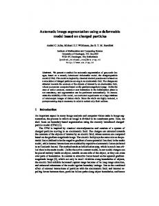
anywhere in a scene. Examples of image classification techniques are [38, 39, 65, 66, 126] among others. There are also many patch-based approaches, which consider pixel information in a fixed-shape subset of the image defined a priori. Boxes or rectangles are a natural shape choice given that pixels are usually arranged in a grid pattern [2, 31, 121]. By placing these shapes in different positions in the image and with different variations of their height, width, orientation and other parameters, the number of pixel subsets to examine becomes tractable. The choice of shapes, however, is largely a matter of convenience. While a square may work well for defining a chessboard, it does a poor job of defining which pixels compose our cheetah. Applications such as digital image editing and robotics demand more precision than a box around an object, they need to know exactly which pixels belong to the object. It would be unacceptable to have a robot reach for the handle of a mug but instead soak its hand in the coffee. Precise object masks are also beneficial for recognizing the identity of an object [72]. Consider the objects in Figure 1.1. A box placed around these objects contains more non-object pixels than object pixels. If we accumulate information over the entire box, the non-object information will certainly dominate, making object recognition difficult. If an image editing program changed the color of the cheetah by making the entire box blue, it would not sell very well. Both the process and applications benefit from accurate object location information. This motivates our goal of recognizing objects and also accurately denoting their pixel masks, termed object recognition and object segmentation.
2. Problem description One possible approach to properly identifying the pixels which belong in an object mask is to learn the shape of the object. There exist a number of top-down methods which attempt to model the outline or silhouette of an object, such as [9, 73,81]. Additional approaches subdivide an object into a number of rigid parts and then model each part’s shape and their relative configuration [12, 41, 67, 82]. These methods show promise for rigid objects, or objects with a small number of rigid 2
2
(a) Image
(b) Bounding box
PROBLEM DESCRIPTION
(c) Object mask
F IGURE 1.1. Examples of (a) images , (b) bounding boxes surrounding objects of interest, and (c) pixel-accuracy object masks.
parts, such as a fire hydrant, or even the side view of a particular breed of horse running. Let us consider, however, all of the objects in Figure 1.2. These objects range from rigid objects such as a car, to extremely deformable objects such as the cheetah with its flexible body and tail in a variety of positions, all the way to objects whose shapes not only change but in fact are uninformative, such as water. These objects have a very large set of shapes they can take, so top-down object knowledge does not sufficiently limit the possible sets of pixels which might make up their object masks. We require a data-driven, or bottom-up approach, which can group together some of the pixels and so reduce the size of the configuration space. For these reasons, there is a growing movement toward using unsupervised image segmentation to provide preliminary pixel grouping [16, 51–53, 68, 86, 88, 91, 93, 94, 111]. Unsupervised image segmentation is a broad term which refers to any 3
CHAPTER 1. INTRODUCTION
Object classes: Bicycle, Bird, Boat, Body, Book, Bottle, Building, Bus, 7 Butterfly species, Car, Chair, Cow, Dining table, Dog, Face, Flower, Grass, Horse, Motorcycle, Person, Plane, Potted plant, Road, Sheep, Sign, Sky, Sofa, Spotted cat, Train, Tree, TV/Monitor, Water
F IGURE 1.2. Examples of the objects we will model throughout this thesis.
method of grouping together pixels which are similar in a feature space. Some of the most common feature spaces are image position, luminance value, color, or the texture in the pixel’s vicinity. Throughout this document we will use some of the more popular segmentation methods, described in Chapter 2, but many other algorithms could be substituted with equal success. 4
3
APPROACH AND DOCUMENT OUTLINE
F IGURE 1.3. Illustration of selecting and combining segmentationgenerated regions to form an object mask.
At the core of our approach is the belief that data-driven bottom-up pixel grouping can be used to define image regions which provide good spatial support for computing image features, and can be used to define the precise location of an object. A simple version of this concept is illustrated in Figure 1.3, where a union of segmentation regions produces an accurate object mask. The goals of this thesis are to define and explore the issues related to, and propose new methods for, combining bottom-up image segmentation and top-down object information to recognize object classes and produce pixel-accurate masks of their locations.
3. Approach and document outline To use image regions generated by unsupervised image segmentation for object recognition, we must first understand the relationship between regions and objects. The most straight-forward method for using image segmentation is as a ‘black box’, grouping the pixels in an image and assuming that each region corresponds to an object that needs to be recognized [94]. In Chapter 3, we propose a set of criteria, experiments, and a quantitative measure of segmentation ‘correctness’ (in joint work with R. Unnikrishnan) that can be used to determine if a segmentation algorithm would be an appropriate black box, as well as comparing the efficacy of multiple algorithms. This work was originally presented in [87, 116, 117]. 5
CHAPTER 1. INTRODUCTION
As a result of experiments conducted using the segmentation algorithms in Chapter 2, we determine that in fact bottom-up image segmentation cannot be used in such a simplistic manner. Our experiments show that segmentation regions rarely correspond perfectly to objects. Instead, they may denote a portion of an object, or they may include both object and non-object pixels. These relationships between segmentation regions and objects, termed over- or under-segmentation, can vary with the algorithm used to create the segmentation, with the algorithm’s parameters, with the image used, in fact they can even vary within an image. These discoveries motivate our approach to using image segmentation for object recognition. Throughout the remainder of this document, we will present a number of object recognition and object segmentation experiments. For ease of reading, we pause in Chapter 4 to describe our experiment methodology and data sets. With our evaluation methodology in place, we can proceed to discuss our approach to incorporating image segmentation into an object recognition system. At the highest level, our approach is to divide an image into regions using bottom-up unsupervised segmentation, describe each region, and then use top-down object knowledge to select and combine the regions to form an object mask. We begin in Chapter 5 by discussing the basis of any object recognition system: image description. Creating an image description involves converting image pixels into features that can be assigned an object label, and in our case the description will be based on the regions created by image segmentation. We present two approaches for representing the image structure within a region. The first is a more traditional representation of repetitive texture [71], which is excellent for discovering objects with distinctive patterns such as cheetah bodies. However, not all objects are composed of repetitive textures. Also, our experiments showed that segmentation-generated regions do not necessarily encompass entire objects, and their extend is subject to the whims of the particular segmentation algorithm and parameters used. Thus, our second representation is the novel Region-based Context Feature (RCF), which considers distinctive image structure in and around a region. By combining the structures around a region based on their scale, not on the region’s area, the RCF
6
3
APPROACH AND DOCUMENT OUTLINE
provides a principled and more stable approach for choosing which structures are relevant to a region. Our bottom-up image segmentation process has proposed groups of pixels which should possess the same object label, and has represented the information in each region in a more practical form. We now require an injection of top-down object information to label which regions and features belong to which object class. Much of the work in generating object masks has relied on fully supervised training data which contains human-drawn object masks. Such training data is extremely expensive to obtain, however, and so the process cannot be scaled to larger object and image sets. Completely unsupervised training data without any object labels can be obtained easily and used for object discovery, but without human input there is no guarantee that the discovered objects will be of interest. In Chapter 6, we learn to classify region features using a training data set of images which are weakly labeled with the objects they contain, but no information is given about the object locations or object masks. Detailed experiments are performed using our region representations and classifier on multiple data sets, testing the relative merits of each representation on different data sets and showing that our approach produces state-of-the-art results. Our object recognition and segmentation framework thus far has implicitly relied on the regions generated by image segmentation to be ‘useful’, large enough to compute higher-order statistics of image structure, but small enough to fall within an object’s boundaries. As we discover in our image segmentation experiments in Chapter 3, this is an unrealistic expectation for a single image segmentation. In Chapter 7, we join [6, 11, 52, 72, 86, 94, 111] in recommending the use of multiple bottom-up segmentations of each image. Unlike [94], however, we believe there is information in all of the segmentations generated by our multiple algorithms and parameters, and we utilize them all in concert to reinforce object recognition and object segmentation. Large regions can provide contextual indications of object presence, regions which lie within object boundaries give object-specific information, and small regions better capture unique local structures. In addition, the correct object boundaries are more likely to be a subset of the union of region
7
CHAPTER 1. INTRODUCTION
F IGURE 1.4. Overview of our algorithm.
boundaries in multiple segmentations rather than in one segmentation. We present experimental evidence of the benefit of using multiple segmentations within our object recognition framework. Given the heterogeneity of the parts of certain objects, such as a person’s shirt and pants, it is possible that even multiple image segmentations may not generate any region which crosses such part boundaries. The Region-based Context Features capture some information from outside of a region, however that information is still local. Chapter 8 considers the potential for improvement by capturing spatial information and enforcing spatial consistency through explicitly modeling the spatial arrangement of an object’s constituent regions. As we discussed earlier, however, many of the objects we wish to model are in fact quite deformable, so a shape-based or part-based method will be too rigid. Instead, we choose to model 8
4
CONTRIBUTIONS
the more flexible constraint of pairwise region adjacency to model spatial relationships, and utilize a random field formulation to enforce spatial consistency. Our publications on region description, classification methods and spatial consistency include [86] and [88]. In summary, this dissertation discovers and addresses a set of challenges related to incorporating image unsupervised segmentation into an object recognition and object segmentation framework. By performing a set of rigorous experiments regarding the relationship between segmentation regions and object masks, we motivate our approach. To address the weaknesses in image segmentation, we create features which better represent regions, utilize multiple segmentations per image, and consider enforcing spatial consistency between region labels. An algorithm overview is given in Figure 1.4. Through these methods we obtain state-of-the-art performance on a number of image data sets. In Chapter 9, we look at the bigger picture by considering some of the applications that could benefit from an object recognition and segmentation system such as ours.
4. Contributions The key contributions of this dissertation include: • A framework for quantitatively evaluating and comparing segmentation algorithms, including: – a quantitative measure of segmentation correctness (in joint work with R. Unnikrishnan), – the definition of criteria for a useful black-box segmentation algorithm and, – a set of experiments to measure those criteria. • Extensive experiments using the above evaluation scheme which elucidate the relationship between segmentation-generated regions and object masks, and motivate our approach to using regions. 9
CHAPTER 1. INTRODUCTION
• A new region descriptor that adapts to the deformable, inconsistent shape of segmentation-generated regions to facilitate object recognition and segmentation. • A framework and thorough experiments for recognizing objects and denoting their pixel masks, trained using only a weakly supervised image set. • An approach to incorporating multiple segmentations into the recognition framework, thereby addressing the issue of image segmentation variability. • A method for describing the spatial relationships between regions and enforcing spatial consistency in the final image labeling to increase robustness and combine heterogeneous object parts.
10
CHAPTER 2
IMAGE SEGMENTATION ALGORITHMS
T
HROUGHOUT
this thesis, a number of unsupervised image segmentation
algorithms will be employed. Although the recognition framework we will introduce is in fact agnostic to the segmentation algorithms used, we
must instantiate our experiments with a set of algorithms. Thus, we begin by introducing the five popular image segmentation algorithms used in this work: mean shift-based segmentation algorithm [25], an efficient graph-based segmentation algorithm [36], a hybrid of the previous two, normalized cuts segmentation using boundaries [44, 76, 104], and expectation maximization [27]. Each of the algorithms has different strengths and weaknesses which we will briefly describe here and then expand upon in Chapter 3.
1. Mean Shift Segmentation The mean shift based segmentation technique was introduced in [25] and is one of many techniques under the heading of “feature space analysis”. The technique is comprised of two basic steps: a mean shift filtering of the original image data (in feature space), and a subsequent clustering of the filtered data points. The filtering step of the mean shift segmentation algorithm consists of analyzing the probability density function underlying the image data in feature space. In the original implementation, the feature space consists of the (x, y) image location of each pixel and the (smoothed) pixel color in L*u*v* space (L∗ , u∗ , v ∗ ). The modes
CHAPTER 2. IMAGE SEGMENTATION ALGORITHMS
of the pdf underlying the data in this feature space will correspond to the locations with highest data density, and data points close to these modes can be clustered together to form a segmentation. The mean shift filtering step consists of finding these modes through the iterative use of kernel density estimation of the gradient of the pdf, and associating with them any points in their basin of attraction. Details may be found in [25]. In the implementations of our object recognition algorithms, we extend the mean shift algorithm to also include texture as a feature. We compute texture using the algorithm from the Berkeley segmentation database website [71, 77] to generate texton histograms; the texton at each pixel is a vector of responses to 24 filters quantized into 30 textons, and the texton histogram centered at a pixel is an accumulation of the textons in a 19x19 pixel window. The low dimensionality of our texton histograms allows for generalization during segmentation, grouping together pixels surrounded by similar but not identical textures. For clarity, our discussion here will only include the spatial and color features. A uniform kernel is used for gradient estimation. The kernel has radius vector h = [hs , hs , hr , hr , hr ], with hs the radius of the spatial dimensions, hr the radius of the color dimensions. For every data point (pixel in the original image) the gradient estimate is computed and the center of the kernel, x, is moved in that direction, iterating until the gradient is below a threshold. This change in position is the mean shift vector. The resulting points have gradient approximately equal to zero, and hence are the modes of the density estimate. Each datapoint is then replaced by its corresponding mode estimate. Finding the mode associated with each data point helps to smooth the image while preserving discontinuities. Let Sxj ,hs ,hr be the sphere in feature space, centered at point x and with spatial radius hs and color radius hr . The uniform kernel has non-zero values only on this sphere. Intuitively, if two points xi and xj are far from each other in feature space, then xi 6∈ Sxj ,hs ,hr and hence xj does not contribute to the mean shift vector and the trajectory of xi will move it away from xj . Hence, pixels on either side of a strong discontinuity will not attract each other.
12
1
MEAN SHIFT SEGMENTATION
However, filtering alone does not provide a segmentation as the modes found are noisy. This “noise” stems from two sources. First, the mode estimation is an iterative process, hence it only converges to within the threshold provided (and with some numerical error). Second, consider an area in feature space larger than Sx,hs ,hr and where the color is uniform or has a gradient of one in each dimension. Since the pixel coordinates are uniform by design, the mean shift vector will be a 0-vector in this region, and the data points in this region will not move and hence not converge to a single mode. Intuitively, however, we would like all of these data points to belong to the same cluster in the final segmentation. For these reasons, mean shift filtering is only a preprocessing step, and a second step is required in the segmentation process: clustering of the filtered data points {x0 }. After mean shift filtering, each data point in the feature space has been replaced by its corresponding mode. As described above, some points may have collapsed to the same mode, but many have not despite the fact that they may be less than one kernel radius apart. In the original mean shift segmentation paper [25], clustering is described as a simple post-processing step in which any modes that are less than one kernel radius apart are grouped together and their basins of attraction are merged. This suggests using single linkage clustering to convert the filtered points into a segmentation. The only other paper using mean shift segmentation that describes the clustering stage is [22]. In this approach, a region adjacency graph (RAG) is created to hierarchically cluster the modes. Also, edge information from an edge detector is combined with the color information to better guide the clustering. This is the method used in the publicly available EDISON system, also described in [22]. The EDISON system, extended to handle texture, is the implementation we use here as our mean shift segmentation system. As we can see in Figure 2.1 and will be further discussed in Chapter 3, the regions generated by mean shift segmentation follow image edges well. The number of regions is not specified, but is instead determined by the bandwidths used and the image data. This makes the number of regions highly variable. The region
13
CHAPTER 2. IMAGE SEGMENTATION ALGORITHMS
sizes may also vary widely as both large and small image features can be captured, although the range is dependant on the position bandwidth.
2. Efficient Graph-based Segmentation Efficient graph-based image segmentation, introduced in [36] by Felzenszwalb and Huttenlocher, is another method of performing clustering in feature space. This method works directly on the data points in feature space, without first performing a filtering step, and uses a variation on single linkage clustering. The key to the success of this method is adaptive thresholding. To perform traditional single linkage clustering, a minimum spanning tree of the data points is first generated (using Kruskal’s algorithm), from which any edges with length greater than a given hard threshold are removed. The connected components become the clusters in the segmentation. The method in [36] eliminates the need for a hard threshold, instead replacing it with a data-dependent term. More specifically, let G = (V, E) be a (fully connected) graph, with m edges {ei } and n vertices. Each vertex is a pixel, x, represented in the feature space. Each edge connects two pixels. The final segmentation will be S = (C1 , ..., Cr ) where Ci is a cluster of data points. The algorithm is: 1. Sort E = (e1 , ..., em ) such that |et | ≤ |et0 | ∀t < t0 � 2. Let S 0 = {x1 }, ..., {xn } , in other words each initial cluster contains exactly one vertex. 3. For t = 1, ..., m (a) Let xi and xj be the vertices connected by et . (b) Let Cxt−1 be the connected component containing point xi on iterai tion t − 1, and li = maxmst Cxt−1 be the longest edge in the minimum i spanning tree of Cxt−1 . Likewise for lj . i (c) Merge Cxt−1 and Cxt−1 if i j k k |et | < min{li + t−1 , lj + t−1 } Cx Cx i j where k is a constant. 4. S = S m 14
3
HYBRID SEGMENTATION ALGORITHM
In contrast to single linkage clustering which uses a constant K to set the threshold on edge length for merging two components, efficient graph-based segmentation uses the variable threshold in (3c). This threshold effectively allows two components to be merged if the minimum edge connecting them does not have length greater than the maximum edge in either of the components’ minimum k . As defined here, τ is dependent on a con|Cxt−1 i | stant k and the size of the component. On the first iteration, li = 0 and lj = 0, and Cx0i = 1 and Cx0j = 1, so k represents the longest edge which will be added
spanning trees, plus a term τ =
to any cluster at any time, k = lmax . As the number of points in a component increases, the tolerance on added edge length for new edges becomes tighter and fewer mergers are performed, thus indirectly controlling region size. However, it is possible to use any non-negative function for τ which reflects the goals of the segmentation system. Intuitively, in the function used here, k controls the final cluster sizes. The merging criterion in (3c) allows efficient graph-based clustering to be sensitive to edges in areas of low variability, and less sensitive to them in areas of high variability. Examples of the efficient graph-based algorithm can be seen in Figure 2.1.
3. Hybrid Segmentation Algorithm An obvious question emerges when describing the mean shift based segmentation method [25] and the efficient graph based clustering method [36]: can we combine the two methods to give better results than either method alone? More specifically, can we combine the two methods to create more stable segmentations that are less sensitive to parameter changes and for which the same parameters give reasonable segmentations across multiple images? In an attempt to answer these questions, the third algorithm we consider is a combination of the previous two algorithms: first we apply mean shift filtering, and then we use efficient graphbased clustering to give the final segmentation. As we will show, it is possible to achieve high-quality segmentations that are less sensitive to their parameters using this approach. Examples of the segmentations generated using this algorithm 15
CHAPTER 2. IMAGE SEGMENTATION ALGORITHMS
are available in Figure 2.1. Regions found by this algorithm are capable of capturing long, ‘wiry’ image structure, however it is also prone to hallucinating wiry structure where there is none.
4. Normalized cuts using boundary maps Another frequently used segmentation algorithm is Normalized Cuts (NCuts) [104]. The normalized cuts algorithm views the image segmentation problem as a graph cut problem. Let the pixels in an image define a weighted graph G = (V, E, W), where the weights W on the edges correspond to the similarity between the pixels joined by that edge (in some feature space). The cut between two sets of pixels A, P B, is cost(A, B) = u∈A,v∈B w(u, v), the total cost of all edges between pixels in A and pixels in B. The segmentation problem can be equated to cutting the graph G into n regions while minimizing the cost of the cuts between them. This, however, can lead to small degenerate regions which are cheap to cut, and other large regions with high variance. To avoid this situation, we can define the association P between a region and the rest of the image to be assoc(A, V ) = u∈A,t∈V w(u, t), and find regions which minimize the cuts in the graph while also maximizing the associativity in the graph. In other words, normalized cuts seeks to minimize: (2.1)
N Cut =
cut(A, B) cut(A, B) + assoc(A, V ) assoc(B, V )
Approximations to the minimal normalized cut can be found by converting the cut problem into a Rayleigh quotient and solving for the second smallest eigenvalue, and clustering the corresponding eigenvectors. To create more than one cut, the process can be repeated iteratively on each region. The graph weights we use in this thesis are computed by inverting the “probability of boundary”, or Pb detector developed by Martin et al. [76]. To predict the likelihood of a boundary between two pixels, the “probability of boundary” Pb classifier considers the difference in brightness, color and texture on either side of the proposed boundary and compares these features to a distribution learned on a database of natural images [77]. 16
5
EM SEGMENTATION ALGORITHM
To implement this procedure, we use the publicly available code by Fowlkes et al. [43, 44, 76]. The nature of regions derived from normalized cuts differs from those created by the other algorithms mentioned here, as can be seen in Figure 2.1. Due to normalizing by the association function, regions are often very similar in size. This has the benefit of creating more regularly-shaped regions, but also the weakness that it is often cheaper to make short cuts in homogeneous regions rather than follow long but correct boundaries. Unlike the other segmentation algorithms discussed, Ncuts must be told exactly how many regions to create and cannot make soft decisions. Finally, while the eigenvalue solution generates two regions in a principled manner, extensions to more than two regions are approximate.
5. EM Segmentation Algorithm As a baseline for the experiments in Chapter 3, we use the classic Expectation Maximization (EM) algorithm [27], with the Bayesian Information Criterion (BIC) to select the number of Gaussians in the model. By minimizing the BIC, we attempt to minimize model complexity while maintaining low error. The BIC is formulated as follows: �
� RSS + g ln(n) BIC = n ln n where n is the sample size, g is the number of parameters, and RSS is the residual sum of squares. As above, the features used are image position (x, y) and pixel color in L*u*v* color space (L∗, u∗, v∗). We present results for the EM algorithm as a baseline for each relevant experiment, however we omit it in the detailed performance discussion. As can be seen in Figure 2.1, the segmentations generated by EM are of much lower quality.
17
CHAPTER 2. IMAGE SEGMENTATION ALGORITHMS
(a) Mean shift segmentation
(b) Efficient graph-based segmentation
(c) Hybrid segmentation algorithm
(d) Normalized cuts segmentation
(e) Expectation maximization-based segmentation F IGURE 2.1. Examples of unsupervised segmentations generated by various algorithms. Segmentations in row (a) were generated by the mean shift-based algorithm, row (b) by the efficient graph-based algorithm, row (c) by the hybrid algorithm, row (d) by normalized cuts, and row (e) by the expectation maximization segmentation algorithm. Each row shows the results of using three different parameters settings.
18
CHAPTER 3
CHARACTERISTICS OF IMAGE SEGMENTATION
I
N
the previous chapter, we described a number of segmentation algorithms
which will be used to generate image regions, and showed examples of such regions. In order to incorporate these regions into an object recognition sys-
tem we need to make a number of decisions regarding which segmentation algorithms to use and how to use them. The easiest approach would certainly be to use segmentation as a ‘black box’ which could outline objects for us. Then the rest of our object recognition system would simply need to recognize the regions generated by our segmentation. The segmentations described in the previous chapter lead us to believe that regions are not guaranteed to properly denote objects, but is this in fact always the case? Were we just unlucky with our parameter choice? If we had found the right parameters for one of the algorithms, would it have been possible to denote the objects in all of the images? If not, how much difference is there between a segmentation region and an object? In this chapter, we propose a quantitative study of segmentation performance. We define a set of characteristics which would allow a segmentation algorithm to be a good ‘black box’, a set of experiments which measure these characteristics and a measure of segmentation accuracy which allows us to perform these experiments. We present an implementation of our evaluation approach by comparing the segmentation algorithms described in the previous chapter. While we find that we can in fact make recommendations about the relative quality of these algorithms as
CHAPTER 3. CHARACTERISTICS OF IMAGE SEGMENTATION
a black box solution, none of the algorithms gives completely satisfactory results. So instead, we use the information gathered from our experiments to motivate our methods for using segmentation regions in the remainder of this thesis.
1. Segmentation Evaluation Framework For a segmentation algorithm to be a useful ’black box’ in a larger system, we propose that it should have three crucial characteristics: 1. Correctness: the ability to produce segmentations which agree with ground truth. That is, segmentations which correctly identify structures in the image at neither too fine nor too coarse a level of detail. 2. Stability with respect to parameter choice: the ability to produce segmentations of consistent correctness for a range of parameter choices. 3. Stability with respect to image choice: the ability to produce segmentations of consistent correctness using the same parameter choice on different images. If a segmentation scheme satisfies these three requirements, then it will give useful and predictable results which can be reliably incorporated into a larger system without excessive parameter tuning. It has been argued that the correctness of a segmentation algorithm is only relevant when measured in the context of the larger system into which it will be incorporated. However, most such systems assume that a segmentation algorithm satisfies a subset of the criteria above. In addition, there is value in weeding out algorithms which give nonsensical results and limiting the list of possible algorithms to those that are well-behaved even if the components of the rest of the system are unknown. It is important to note that a segmentation algorithm can provide useful segmentations despite not meeting the criteria listed here, however the segmentation algorithm could not act as a black box. If a segmentation algorithm is weak in any of the above criteria, the larger system would have to make allowances. For example, if an algorithm is not stable with respect to image choice, one could segment each image with multiple parameters, raising the probability that object boundaries are 20
1
SEGMENTATION EVALUATION FRAMEWORK
captured in at least one segmentation. This is in fact our approach, which will be discussed later in this chapter and thesis. Thus, in addition to discussing which segmentation algorithm provides the best black box, we will use our experiments to motivate our approach to incorporating segmentation into our object recognition framework. To evaluate a segmentation algorithm for the above characteristics, we perform a set of experiments on a database of images which have ground truth segmentations, namely the Berkeley segmentation database [77]. For each image in this database, there are roughly 5-7 ground truth human segmentations to which to compare machine-generated segmentations, with examples given in Figure 3.1. To test an algorithm for each characteristic listed above, we will perform the following experiments, with numbers corresponding to each characteristic: 1. To measure the correctness of an algorithm, we will generate multiple segmentations of each image in the database with multiple parameter settings. For each image, the segmentation that best corresponds to the ground truth is an approximation of the best performance possible by the algorithm. 2. To measure the stability of an algorithm with respect to parameter choice, we must once again segment each image with multiple parameters. If the segmentation quality differs substantially with different parameters, then the algorithm is unstable. 3. To measure the stability of an algorithm with respect to image choice, we segment all of the images in the database with the same parameters. If the segmentation quality differs substantially between images, then the algorithm is unstable. Many past evaluations of segmentation performance have been merely qualitative. In contrast, we wish to perform a quantitative evaluation, so we require a measure of the accuracy of an image segmentation compared to its ground truth. In order to effectively carry out the experiments suggested, the measure must be able to compare a segmentation against multiple ground truth human segmentations. In
21
CHAPTER 3. CHARACTERISTICS OF IMAGE SEGMENTATION
F IGURE 3.1. Examples of images from the Berkeley image segmentation database [77] with five of their human segmentations. Note the variation in region refinement between the human segmenters.
addition, it must not have any degenerate cases in which a particular segmentation, (such as every pixel belonging to a separate region), is given an artificially high score. Next, since we wish to compare multiple segmentations of the same image, as well as segmentations of different images, the measure cannot make any assumptions about how the regions are generated, nor the number or size of the regions. Since we also wish to compare to multiple ground truth segmentations which may agree or disagree in different image areas, it would be beneficial if the measure could adaptively accommodate to the level of agreement over the image. Note that in the human segmentations in Figure 3.1, there are some image areas where all of the ground truth segmentations are in agreement, and other areas where there are varying levels of disagreement. Finally, it is important that the score generated by the measure be easily interpretable and comparable across images. In the next section, we introduce the Normalized Probabilistic Rand index, a measure of segmentation accuracy which does indeed meet all of these criteria. 22
2
NPR MEASURE
2. NPR measure In [115], Unnikrishnan and Hebert introduce a measure for evaluating the similarity of a novel segmentation to a set of ground truth image segmentations, the Probabilistic Rand (PR) Index. The original Rand Index [92], a popular nonparametric measure, measures the agreement between two segmentations as a function of the number of pairs of points whose label (or region) relationships agree in both segmentations. In other words, if two points belong to the same region in one segmentation, they should also belong to the same region in the other segmentation. The same holds true if the two points belong to different regions. Formally, let X = {xi }, i = 1..N be a set of points, and S and S 0 two segmentations of those points. Let li be the label, or region, of point xi in segmentation S, and li0 the label in segmentation S 0 . The Rand Index is the fraction of pairs of points whose relationships agree in both segmentations, computed as: (3.1)
R(S, S 0 ) =
� � � 1 X � 0 0 0 0 I l = l ∧ l = l + I l = 6 l ∧ l = 6 l � i j i j i j i j N 2
i,j i6=j
where Iis an indicator function. Notice the lack of reference to which region a pair of points belongs. Also, S and S 0 may have different numbers of regions. If S 0 = Stest is a novel segmentation and S is a human segmentation, the Rand Index gives the correctness of segmentation S 0 . The Probabilistic Rand (PR) index extends the Rand Index to handle multiple ground truth segmentations. Let {S1 , ..SK } be a set of ground truth segmentations for image X = {xi }, and liSk the label of pixel xi in segmentation Sk . Define pij to be the probability that xi and xj are given the same label over all consistent human segmentations of the image. The PR index is defined as: (3.2) PR(Stest , {Sk }) =
� � � �� i 1 X h � Stest Stest Stest Stest I l = l p + 1 − I l = l (1 − p ) � ij ij i j i j N 2
=
i,j i