Subcarrier Domain of Multicarrier Continuous-Variable Quantum Key

Subcarrier Domain of Multicarrier Continuous-Variable Quantum Key Distribution Laszlo Gyongyosi 1

Quantum Technologies Laboratory, Department of Telecommunications Budapest University of Technology and Economics 2 Magyar tudosok krt, Budapest, H-1117, Hungary 2 MTA-BME Information Systems Research Group Hungarian Academy of Sciences 7 Nador st., Budapest, H-1051, Hungary [email protected]

Abstract We propose the subcarrier domain of multicarrier continuous-variable (CV) quantum key distribution (QKD). In a multicarrier CVQKD scheme, the information is granulated into Gaussian subcarrier CVs and the physical Gaussian link is divided into Gaussian subchannels. The sub-channels are dedicated for the conveying of the subcarrier CVs. The angular domain utilizes the phase-space angles of the Gaussian subcarrier CVs to construct the physical model of a Gaussian sub-channel. The subcarrier domain injects physical attributes to the description of the subcarrier transmission. We prove that the subcarrier domain is a natural representation of the subcarrier-level transmission in a multicarrier CVQKD scheme. We also extend the subcarrier domain to a multiple-access multicarrier CVQKD setting. We demonstrate the results through the adaptive multicarrier quadrature-division (AMQD) CVQKD scheme and the AMQD-MQA (multiuser quadrature allocation) multiple-access multicarrier scheme. The subcarrier domain representation provides a general apparatus that can be utilized for an arbitrary multicarrier CVQKD scenario. The framework is particularly convenient for experimental multicarrier CVQKD scenarios. Keywords: quantum key distribution, continuous-variables, CVQKD, AMQD, AMQDMQA, quantum Shannon theory.

1

1 Introduction The continuous-variable quantum key distribution protocols allow for the parties to establish an unconditionally secure communication over the traditional telecommunication networks. In comparison to discrete-variable (DV) QKD, the CVQKD schemes do not require single-photon devices, a fact that allows us to implement in practice by standard devices [1–10], [24–31]. Despite the several attractive benefits of CVQKD, these protocols still require significant performance improvements to be comparable with that of the traditional telecommunications. For this purpose, the multicarrier CVQKD has been recently introduced through the adaptive multicarrier quadrature division (AMQD) modulation [2]. In a multicarrier CVQKD system, the Gaussian input CVs are granulated into subcarrier Gaussian CVs via the inverse Fourier transform, which are decoded by the receiver by the unitary CVQFT (continuous-variable quantum Fourier transform) operation [2]. Precisely, the multicarrier transmission divides the physical Gaussian link into several Gaussian sub-channels, where each sub-channel is dedicated for the conveying of a Gaussian subcarrier CV. In particular, the multicarrier transmission injects several benefits to CVQKD, such as improved secret key rates, higher tolerable excess noise, and enhanced transmission distances. Specifically, the benefits of the multicarrier CVQKD modulation has been extended to a multiple-access CVQKD through the AMQD-MQA (multiuser quadrature allocation) scheme [3], in which the simultaneous reliable transmission of the legal users is handled through the sophisticated allocation mechanism of the Gaussian subcarriers. The SVD-assisted (singular value decomposition) AMQD injects further extra degrees of freedom into the transmission [4], which can also be exploited in a multiple-access multicarrier CVQKD [5–7]. Here, we provide a natural representation of the subcarrier CV transmission and show that it also allows us to utilize the physical attributes into the sub-channel modeling. The angular domain representation is a useful tool in traditional telecommunications to model the physical signal propagation through a communication channel. The angular domain representation is aimed at revealing and verifying the connections of the physical layer and the mathematical channel model in different scenarios, avoiding the use of an inaccurate channel representation [21–23]. Here, we show that similar benefits can be brought up to multicarrier CVQKD. We define the subcarrier domain representation for multicarrier CVQKD. The subcarrier domain utilizes the phase-space angles of the Gaussian subcarrier CV to construct the model of a Gaussian sub-channel and to build an appropriate statistical model of subcarrier transmission. The subcarrier domain is an adequate application for multicarrier CVQKD since it is a natural representation of the CVQFT operation. The key behind the subcarrier domain representation is the Fourier operation, which has a central role in a multicarrier CVQKD setting since this operation makes possible the construction of Gaussian subcarrier CVs from the single-carriers and Gaussian sub-channels from the physical Gaussian link. Particularly, the CVQFT transformation not just opens the door for the characterization of the subcarrier domain of a Gaussian sub-channel but also provides us a framework to study the effects of psychical layer transmission in an experimental multicarrier CVQKD scenario. The subcarrier domain utilizes physical attributes such as the phase space angle into the description of

2

the transmission. Thus, the subcarrier domain representation takes into account not just the theoretical model but also the physical level of the subcarrier transmission. Since the subcarrier domain is a natural representation of a multicarrier CVQKD transmission, it allows us to extend it to a multiple-access multicarrier CVQKD setting. Furthermore, the subcarrier domain model provides a general framework for any experiential multicarrier CVQKD. This paper is organized as follows. In Section 2, some preliminaries are briefly summarized. Section 3 discusses the subcarrier domain representation for multicarrier CVQKD. Section 4 extends the subcarrier domain for multiple-access multiuser CVQKD. Finally, Section 5 concludes the results. Supplemental information is included in the Appendix.

2 Preliminaries In Section 2, we briefly summarize the notations and basic terms. For further information, see the detailed descriptions of [2–6].

2.1 Basic Terms and Definitions 2.1.1 Multicarrier CVQKD In this section we very briefly summarize the basic notations of AMQD from [2]. The following description assumes a single user, and the use of n Gaussian sub-channels  i for the transmission of the subcarriers, from which only l sub-channels will carry valuable information. In the single-carrier modulation scheme, the j-th input single-carrier state j j = x j +ip j

is a

Gaussian state in the phase space  , with i.i.d. Gaussian random position and momentum quad-

(

ratures x j Î  0, sw2

0

),

(

p j Î  0, sw2

0

) , where

sw2 is the modulation variance of the quadra0

tures. In the multicarrier scenario, the information is carried by Gaussian subcarrier CVs,

fi = x i +ipi , x i Î  ( 0, sw2 ) , pi Î  ( 0, sw2 ) , where sw2 is the modulation variance of the

subcarrier quadratures, which are transmitted through a noisy Gaussian sub-channel  i . Precisely, each  i Gaussian sub-channel is dedicated for the transmission of one Gaussian subcarrier CV from the n subcarrier CVs. (Note: index l refers to the subcarriers, while index j, to the single-carriers, throughout the manuscript.) The single-carrier state j j in the phase space  can be

modeled as a zero-mean, circular symmetric complex Gaussian random variable æ ö 2ù é z j Î  ççç 0, sw2 ÷÷÷ , with variance sw2 =  ê z j ú , and with i.i.d. real and imaginary zero-mean zj ø zj è ë û

(

Gaussian random components Re ( z j ) Î  0, sw2

0

) , Im ( z

j

) Î  ( 0, sw2

0

).

In the multicarrier CVQKD scenario, let n be the number of Alice’s input single-carrier Gaussian states. Precisely, the n input coherent states are modeled by an n-dimensional, zero-mean, circular symmetric complex random Gaussian vector

3

T

z = x + ip = ( z1, , z n ) Î  ( 0, Kz ) ,

(1)

where each z j is a zero-mean, circular symmetric complex Gaussian random variable

æ z j Î  ççç 0, sw2 zj è

÷÷ö , z = x + ip . j j ÷ø j

(2)

In the first step of AMQD, Alice applies the inverse FFT (fast Fourier transform) operation to vector z (see (1)), which results in an n-dimensional zero-mean, circular symmetric complex T

Gaussian random vector d , d Î  ( 0, Kd ) , d = (d1, , dn ) , precisely as

d=F

-1

(z) = e

dT AAT d 2

(

=e

where

s2 d12 ++dn2 w0

) ,

2

(

(3)

)

di = xd + ipd , di Î  0, sd2 , i

i

i

(4)

é 2ù where sw2 =  ê di ú and the position and momentum quadratures of fi di ë û random variables

(

)

(

are i.i.d. Gaussian

)

Re ( di ) = xd Î  0, sw2 , Im ( di ) = pd Î  0, sw2 , i

i

i

i

(5)

T ù é where Kd =  éê dd† ùú ,  éë d ùû =  éê e ig d ùú = e ig éë d ùû , and  éê ddT ùú =  ê e ig d (e ig d ) ú = e i2 g éê ddT ùú ë û ë û ë û ë û êë ûú for any g Î éë 0, 2p ùû .The T (  ) transmittance vector of  in the multicarrier transmission is T T (  ) = éëT1 (  1 ) , ,Tn (  n ) ûù Î  n ,

(6)

where

Ti (  i ) = Re (Ti (  i ) ) + i Im (Ti (  i ) ) Î  ,

(7)

is a complex variable, which quantifies the position and momentum quadrature transmission (i.e., gain) of the i-th Gaussian sub-channel  i , in the phase space  , with real and imaginary parts

0 £ Re Ti (  i ) £ 1

2 , and 0 £ Im Ti (  i ) £ 1

2.

(8)

Particularly, the Ti (  i ) variable has the squared magnitude of

Ti (  i )

2

2

2

= Re Ti (  i ) + Im Ti (  i ) Î  ,

(9)

where

ReTi (  i ) = Im Ti (  i ) .

(10)

The Fourier-transformed transmittance of the i-th sub-channel  i (resulted from CVQFT operation at Bob) is denoted by 2

F (Ti (  i ) ) .

4

(11)

2 The n-dimensional zero-mean, circular symmetric complex Gaussian noise vector D Î  ( 0, sD )

n

of the quantum channel  , is evaluated as T

D = ( D1, , Dn ) Î  ( 0, KD ) ,

(12)

where

KD =  éê DD† ùú , û ë with independent, zero-mean Gaussian random components

(

)

(13)

(

Dx Î  0, s 2 , and Dp Î  0, s 2 i

i

i

i

),

(14)

with variance s 2 , for each Di of a Gaussian sub-channel  i , which identifies the Gaussian i

noise of the i-th sub-channel  i on the quadrature components in the phase space  . The CVQFT-transformed noise vector can be rewritten as T

F ( D ) = ( F ( D1 ) , , F ( Dn ) ) , with independent components F ( Dx

i

) Î  ( 0, sF2 (  ) ) i

and F ( Dp

i

(15)

) Î  ( 0, sF2 (  ) )

on the quad-

i

ratures, for each F ( Di ) . Precisely, it also defines an n-dimensional zero-mean, circular symmet-

(

)

ric complex Gaussian random vector F ( D ) Î  0, KF ( D ) with a covariance matrix †ù é KF ( D ) =  ê F ( D ) F ( D ) ú . ë û

(16)

3 Subcarrier Domain of Multicarrier CVQKD Proposition 1 (Subcarrier domain representation of multicarrier transmission.) For the i-th Gaussian sub-channel  i , the subcarrier domain representation is f (Ti (  i ) ) = UTi (  i )U , i

where U is the CVQFT operator. Proof. The proofs throughout assume l Gaussian sub-channels for the multicarrier transmission. The angles of the fi transmitted and the fi¢ received subcarrier CVs in the phase space  are denoted by qi* Î éë 0, 2p ùû , and qi Î éë 0, 2p ùû , respectively. Specifically, first, we express F ( T (  ) ) as

F ( T (  )) =

å F (Ti (  i )) l l -1 l -1

=

å å Tke i =0 k =0

from which F (Ti (  i ) ) is yielded as 5

- i 2 pik l

(17)

,

l -1

å Tke

F (Ti (  i ) ) =

- i 2 pik l

.

(18)

k =0

Next, we recall the attributes of a multicarrier CVQKD transmission from [2]. In particular, assuming l Gaussian sub-channels, the output y is precisely as follows:

y = F ( T (  )) F ( d ) + F ( D )

= F ( T (  ) ) F ( F -1 ( z ) ) + F ( D ) = ( F ( T (  )) F ) d + F ( D ) = å F (Ti (  i ) ) di + F ( Di ),

(19)

l

where

F ( d ) = F ( F -1 ( z ) ) = z .

(20)

The l columns of the l ´ l unitary matrix F formulate basis vectors, which are referred to as the domain f , from which the subcarrier domain representation f (Ti (  i ) ) of Ti (  i ) is dei

i

fined as

f (Ti (  i ) ) = F (Ti (  i ) ) F , i

(21)

Thus, (19) can be rewritten as

y

f

= f ( T (  =

å f

i

l

where y

f

)) d + F ( D ) (Ti (  i ) )di + F ( Di ),

(22)

is referred to as the subcarrier domain representation of y .

Particularly, from (21) follows that f (Ti (  i ) ) can be expressed as i

f (Ti (  i ) ) = UTi (  i )U , i

(23)

where U is an l ´ l unitary matrix as (24) U =F, where F refers to the CVQFT operator which for l subcarriers can be expressed by an l ´ l matrix, as

U =

1 l

e

-i 2 pik l

, i, k = 0, , l - 1 ,

(25)

Thus, l

åU (Ti (  i )) .

f ( T (  ) ) = i

(26)

i =1

To conclude, the results in (17) and (18) can be rewritten as l

åU (Ti (  i ))

(27)

F (Ti (  i ) ) = U (Ti (  i )) .

(28)

U ( T (  )) =

i =1

thus, Specifically, an arbitrary distributed f ( T ( 

))

following statistics: 6

can be approximated via an averaging over the

(

 ( f ( T (  ) ) ) Î  0, sT2

( )

),

(29)

by theory. Since the unitary U operation does not change the distribution of  ( T (  ) ) , an arbitrarily distributed T (  ) can be approximated via an averaging over the statistics of

 (T( 

) ) Î  ( 0, sT2 (  ) ) .

(30) ■

Theorem 1 (Subcarrier domain of a Gaussian sub-channel). The f subcarrier domain reprei

sentation of  i , i = 0 l - 1 , is f (Ti (  i ) ) = i

†

†

å k A ( i )b ( k l ) b ( cos qi )b ( cos qi* ) b ( i l ) ,

k = 0 l - 1 , where b ( ⋅ ) is an orthonormal basis vector of f , qi* and qi are the phase-space i

angles of fi

and fi¢ , A (  i ) = x i , where x i is a real variable, x i ³ 0 .

Proof. The b basis vectors of f are evaluated as follows: Let qi* Î éë 0, 2p ùû refer to the angle of the i-th i noise-free input Gaussian subcarrier CV fi in  . The angle of the i-th noisy subcarrier CV

fi ¢

is referred to as qi Î éë 0, 2p ùû , qi ¹ qi* .

In particular, for the subcarrier domain representation, the scaled CVQFT operation defines the b ( ⋅ ) basis at l Gaussian sub-channels as an l ´ 1 matrix:

æ 1 çç çç e -i2p cos qi çç 1 ç b ( cos qi ) = çç e-i2p 2 cos qi lç çç  çç çe-i2p (l -1 ) cos qi çè

÷÷ö ÷÷ ÷÷ ÷÷ ÷÷ . ÷÷ ÷÷ ÷÷ ÷÷ ø

(31)

æ 1 ÷÷ö çç * çç -i2p cos qi ÷÷ ÷÷ çç e ÷÷ * ç b ( cos qi* ) = 1 çç e -i2p 2 cos qi ÷÷÷ . lç ÷÷ çç ÷÷  çç çç -i2p (l -1 ) cos qi* ÷÷÷ ÷ø çèe

(32)

while for the input angle qi* also defines an l ´ 1 matrix as

Precisely, the difference of the cos functions of the i-th qi* transmitted and the qi received angles is defined as ti = cos qi - cos qi* .

7

(33)

Let b ( cos qi ) and b ( cos qi* ) be the basis vectors of cos qi , cos qi* [21–23], then for the

Wi = qi - qi* angle †

cos Wi = b ( cos qi* ) b ( cos qi ) ,

(34)

cos Wi = f ( ti ) ,

(35)

and where [21]

f ( ti ) = 1l e

(

ip ( l -1 ) cos qi -cos qi*

) sin( pl ( cos qi -cos qi* )) . sin( p ( cos qi -cos qi* ) )

(36)

In particular, using (36), after some calculations, the result in (34) can be rewritten as

( ( ( (

sin pl cos qi -cos qi*

cos Wi =

l sin p cos qi -cos qi*

)) . ))

Specifically, by expressing (36) via the formula of sinc ( x ) = sin ( px ) p1x ,

(37)

(38)

one can find that for l  ¥ , f ( ti ) can be rewritten as [21]

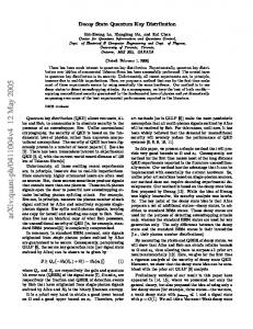
lim f ( ti ) = e ipl ti sinc ( l ti ) .

l ¥

(39)

The function f ( ti ) for different values of ti is depicted in Fig. 1. The function picks up the

f ( ti ) = 1 maximum at ti = 0 , with a period r = 1 . For l sub-channels, a period yields l values.

Figure 1. The function f ( ti ) (blue) for different values of ti . The period of the function is

r = 1 . The sinc function (green) is approximated with an arbitrary precision in the asymptotic limit of l  ¥ . Next, we utilize function f ( ⋅ ) to derive the f subcarrier domain representation of  i . Funci

tion f ( ti ) at a given qi formulates a plot

8

p : ( cos qi , f ( ti ) ) ,

(40)

where from the r = 1 periodicity of f ( ⋅ ) follows that the main loops are obtained at

cos qi = cos qi* .

(41)

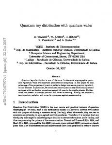
The plot f ( ti ) as a function of cos qi is depicted in Fig. 2, for qi* = p 2 , l = 2 .

Figure 2. The f subcarrier domain representation of  i , at qi* = p 2 , l = 2 . The function i

f ( ti ) picks up the maximum at ti = 0 . From the bases b ( ⋅ ) of (31) and (32), the Fourier bases b ( kl ) and b ( li ) , i, k = 0, , l - 1 is defined as follows: The set Sb of the f orthonormal basis over the  l complex space of the f subcarrier domain representation can be defined as and b ( kl ) is an l ´ 1 matrix as

Sb = {b ( 0 ) , b ( 1l ), , b ( l -l 1 ) } Î  l ,

æ 1 ö÷ çç ÷ çç 1 ÷÷ ç ÷÷÷ 1 ç b ( 0 ) = çç 1 ÷÷÷ , and b ( kl ) = lç ÷ çç  ÷ çç ÷÷÷ çç 1 ÷÷ è ø while the b ( li ) l ´ 1 matrix is precisely as

9

æ 1 ö÷ çç ÷ çç -i2l pk ÷÷ ÷÷ çç e çç -i2 p 2k ÷÷÷ 1 ç e l ÷÷÷ , lç çç ÷÷ çç  ÷ çç -i2 p(l -1)k ÷÷÷ ÷ çe l çè ø÷÷

(42)

(43)

æ 1 ÷ö çç ÷ çç -il2 pi ÷÷ ÷÷ e çç çç -i2 pi 2 ÷÷÷ b ( li ) = 1 çç e l ÷÷ . ÷÷ lç çç  ÷÷ çç ÷ çç -i2 pi(l -1) ÷÷÷ çèe l ÷÷ø

(44)

Precisely, using the orthonormal basis of (42), the result in (36) can be rewritten as †

f ( ti ) = b ( 0 ) b ( ti ) .

(45)

Specifically, the expression of (45) allows us to redefine the plot of (40) to express b ( kl ) as follows:

pb ( k ) : ( cos qi , f ( cos qi - kl ) ),

(46)

l

and thus the maximum values are obtained at

cos qi =

k l

.

(47)

Particularly, at a given l, evaluating f at k = 1, , l - 1 yields the following values [21]:

and

f ( kl ) = 0,

(48)

f ( -lk ) = f ( l -l k ) .

(49)

In particular, the A (  i ) parameter is called the virtual gain of the  i sub-channel transmittance coefficient, and without loss of generality, it is defined as A (  i ) = xi ,

(50)

where x i is a real variable, x i ³ 0 . From (31), (32), and (50), T (  ) can be expressed as

T(  ) =

l -1

†

å A (  i )b ( cos qi )b ( cos qi* )

.

(51)

i =0

By exploiting the properties of the Fourier transform [21–23], for a given cos qi* and cos qi ,

f ( T (  ) ) can be rewritten as f ( T (  ) ) =

=

l -1 l -1

†

å å b ( kl ) Ti (  i )b ( li ) i =0 k =0 l -1 l -1

†

i =0 k =0 l -1 l -1

=

†

å å b ( kl ) A (  i )b ( cos qi )b ( cos qi* ) b ( li )

(52)

†

å å xib ( kl ) b ( cos qi )b ( cos qi* ) b ( li ). †

i =0 k =0

†

Specifically, in (52), for the representation of term b ( cos qi* ) b ( i l ) [21], set S for the f domain of  i as i

10

f

i

can be defined

S

The set S

f

f

: cos qi - ( kl ) < 1l .

(53)

in the subcarrier domain representation for qi* = p 2 , l = 2 and k = 0, , l - 1 is

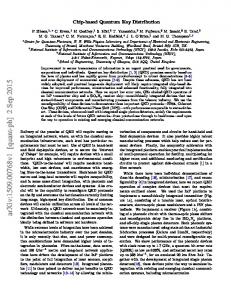
illustrated by the dashed area in Fig. 3. The b ( 0 ) , b ( 1l ), , b ( l -l k ) basis vectors of f for l = 2 are also depicted, evaluated via (46).

Figure 3. The set S

f

(dashed areas) for qi* = p 2 , l = 2 Gaussian sub-channels and

k = 0, l - 1 . The curves (red, green) depict the basis vectors b ( 0 ) , b ( 1l ) of f . Putting the pieces together, from (52), f (Ti (  i ) ) of a given Gaussian sub-channel  i is i

yielded as follows:

f (Ti (  i ) ) i

l -1

=

†

å b ( kl ) Ti ( i )b ( li )

k =0 l -1

=

(54) †

å A ( i )b ( kl ) b ( cos qi )b ( cos qi* ) b ( li ). †

k =0

■

3.1 Statistics of Subcarrier Domain Sub-channel Transmission Theorem 2 (Transmittance of the Gaussian sub-channels). For arbitrary qi* , the magnitude

f (Ti (  i ) ) i

of f (Ti (  i ) ) of a given  i is maximized in the asymptotic limit of i

cos Wi  1 , where Wi = qi - qi* . Averaging over the statistics  ( f ( T (  rank (  ( f ( T (  ) ) ) ) = min ( Si , Sk ber of non-zero rows and columns of

) , where the cardinality of sets f ( T (  ) ) . i

11

) ) ) Î  ( 0, sT2 (  ) ) ,

Si , Sk identifies the num-

Proof. First, we recall f (Ti (  i ) ) from (54) and express f (Ti (  i ) ) as i

i

l -1

†

å xib ( kl ) b ( cos qi )b ( cos qi* ) b ( li ) .

f (Ti (  i ) ) = i

†

(55)

k =0

For a given qi* , the values of angle qi has the following statistical impacts on (55). Without loss of generality, let parameters i and k be fixed as i, k = {C ,C } ,

(56)

where C > 0 is a real variable. Particularly, for the  i sub-channels, the f (Ti (  i ) ) magnitudes formulate a set i

¶=

{ f (Ti (  i )) ,i = 0, , l - 1} .

(57)

Wi = qi - qi* ,

(58)

i

Let and let s be the number of sub-channels for which f (Ti (  i ) ) » 0 . i

Specifically, for ¶ , let determine Wi the value of k as ì k Î é 0, 2C ù , if Wi  p üï ï ë û ïý . k =ï í ï = = W = , 0 k i C if i ï ïþï î Let us define a 0 initial subset with 0 = s 0 , as

0 =

{

(Tj (  j ) ) , j

fj

(59)

}

= 0, , s 0 - 1 Í ¶,

(60)

where

f (Tj (  j ) ) » 0. j

(61)

In this setting, as cos Wi  1 , the cardinality of  increases,

 : cos Wi  1 :  = s > 0 = s 0 ,

(62)

while as cos Wi  -1 , the cardinality of  decreases, thus

 : cos Wi  -1 :  = s < 0 = s 0 .

(63)

In particular, as (63) holds, the range of k expands from C to the full domain of k = éë 0, 2C ùû , and

f (Ti (  i ) ) decreases, thus i

f (Ti (  i ) ) » a, i

(64)

where a is an average which around the f (Ti (  i ) ) coefficients stochastically moves [21–23]. i

The impact of cos Wi  -1 on

f (Ti (  i ) ) i

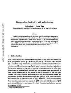
is depicted in Fig. 4 for i, k = {C ,C } ,

i = C = 0.5l . The maximum transmittance is normalized to unit for k = 0.5C . Statistically, the convergence of cos Wi  -1 improves the range of k and decreases the sub-channel transmittance (see (59)).

12

Figure 4. The impact of cos Wi  -1 on f (Ti (  i ) ) for a fixed i = C = 0.5l on a subi

channel  i . The parameter range changes to i, k = {C , éë 0, 2C ùû } , C = 0.5l , from i, k = {C ,C } . For cos Wi  1 , the transmittance picks up the maximum at k = C = 0.5l (red) in a narrow range of k » C . Statistically, as cos Wi  -1 , the transmittance significantly decreases, moving stochastically around an average a (dashed grey line) within the full range k = éë 0, 2C ùû . Particularly, the degrees of freedom in f ( T (  ) ) can be evaluated through the rank of f ( T ( 

)) .

Let us identify the number of non-zero rows and columns of f ( T (  ) ) via Si i

sets Si , Sk , respectively. By averaging [21–23] over the statistics of

(

 ( f ( T (  ) ) ) Î  0, sT2

( )

),

and Sk , of

(65)

thus the rank of  ( f ( T (  ) ) ) without loss of generality is expressed as

rank (  ( f ( T (  ) ) ) ) = min ( Si , Sk

)

» min ( å l cos qi , å l cos qi* ),

(66)

for an arbitrary distribution, by theory [21]. The rank in (66) basically changes in function of the number l of  i Gaussian sub-channels utilized for the multicarrier transmission since the increasing l results in more non-zero elements in  ( f ( T (  ) ) ) [21–23]. On the other hand, the rank in (66) also changes in function of qi . Specifically, as cos Wi  1 , the matrix  ( f ( T (  ) ) ) will have significantly decreased number of non-zero entries (see (62)), while for cos Wi  -1 , the rank increases because the number of nonzero entries in (66) increases [21] (see (63)). These statements can be directly extended to the diversity, since the div ( ⋅ ) diversity function of

 ( f ( T (  ) ) ) is evaluated via the number of non-zero entries in  ( f ( T (  ) ) ) ,

13

div (  ( f ( T ( 

( i, k )

where Ei,k identifies an

) ) ) ) =  Ei,k (  ( f ( T (  ) ) ) ) ¹ 0 ,

(67)

" i ,k

entry of  ( f ( T (  ) ) ) . Precisely, from (67) follows that

div (  ( f ( T (  ) ) ) ) increases with the number l of Gaussian sub-channels. ■

4 Subcarrier Domain of Multiuser Multicarrier CVQKD Lemma 1 (Subcarrier domain of multiple-access multicarrier CVQKD). The f ( T (  ) ) of T( 

)

K ,Kout

in a Kin , Kout multiuser setting is f in

a Kout ´ Kout unitary U K

out

=

1 Kout

( T (  )) = U K

out

T (  )U K

out

, where U K

out

is

-i 2 pik

e Kout , i, k = 0, , Kout - 1 .

Proof. Let Kin , Kout be the number of transmitter and receiver users in a multiple access multicarrier CVQKD [3], and let Z be the Kin dimensional input of the Kin users. The Gaussian CV subcarriers formulate the Kin dimensional vector

D = UK Z ,

(68)

in

where U K The U K

in

in

stands for the inverse CVQFT unitary operation.

and U K

out

, K in ´ K in , Kout ´ Kout unitary matrices at l Gaussian sub-channels are as

follows:

UK

in

=

1 Kin

=

1 Kout

i 2 pik

e Kin , i, k = 0, , Kin - 1 ,

(69)

and

UK

out

-i 2 pik

e Kout , i, k = 0, , Kout - 1 ,

(70)

which unitary is the CVQFT operation. (For further details, see the properties of the multicarrier CVQKD modulation in [2] and [3–6].) Specifically, the output Y in a Kin , Kout setting is then yielded as

Y = U K T (  ) (U K D ) + U K D out

= (U K T (  )U K out

=

K ,K f in out

out

out

out

) D + UK

( T (  )) D + U K

out

out

D

(71)

D,

thus without loss of generality K ,Kout

f in K ,Kout

Particularly, by rewriting (52), f in

( T (  )) = U K

( T (  ))

14

out

T (  )U K

can be expressed as

out

.

(72)

K ,Kout

f in

( T (  )) = = = =

Kin -1 Kout -1

†

out

( kl ) Ti (  i )bK ( li )

out

( kl ) A (  i )bK ( cos qi )bK ( cos qi* ) bK ( li )

å å

bK

å å

bK

å å

x ibK

i =0 k =0 Kin -1 Kout -1 i =0 k =0 Kin -1 Kout -1 i =0

k =0

in

†

†

out

in

in

†

( kl ) bK ( cos qi )bK ( cos qi* ) bK ( li ), †

out

(73)

out

in

in

where the basis vectors are precisely as

bK

out

( cos qi ) =

1 Kout

æ 1 çç i 2 p l cos qi çç çç e Kout çç -i 2 p 2l cos qi çç çç e Kout çç  çç çç -i2 p( Kout -1)l cos qi çç Kout çèe

ö÷ ÷÷ ÷÷ ÷÷ ÷÷ ÷ ÷÷÷ , and bKin ( cos qi* ) = ÷÷ ÷÷ ÷÷ ÷÷ ÷ ø÷

æ 1 çç çç -i 2 pl cos qi* çç e Kin çç çç -i2 p 2l cos qi* çç e Kin çç çç  çç çç -i2 p( Kin -1)l cos qi* Kin ççe è

1 Kin

÷÷ö ÷÷ ÷÷ ÷÷ ÷÷ ÷÷ ÷÷ , ÷÷ ÷÷ ÷÷ ÷÷ ÷÷ ÷ø

(74)

thus

bK

out

( kl ) =

1 Kout

æ ö÷ 1 çç ÷÷ -i 2 pk çç ÷÷ çç e Kout ÷÷ ÷÷ çç -i2 p 2k ÷÷ , and b çç Kout e ÷÷ Kin çç ÷÷ çç  ÷÷ çç çç -i2 p( Kout -1)k ÷÷÷ ÷ ççèe Kout ø÷

( li ) =

æ ö÷ 1 çç ÷÷ -i 2 pi çç ÷÷ çç e Kin ÷ çç -i2 pi 2 ÷÷÷ ÷÷ . çç Kin ÷÷ çç e ÷÷ çç  ÷÷ çç çç -i2 pi ( Kin -1) ÷÷÷ ÷ ççèe Kin ø÷

1 K in

(75)

Without loss of generality, the function f from (36) can be rewritten as f

Kout

( ti ) =

1 Kout

ipl ( Kout -1 )ti

e

Kout

sin( pl ti )

(

sin p

l Kout

ti

)

,

(76)

with

cos Wi =

( (

sin pl cos qi -cos qi*

(

Kout sin p

( cos qi -cos qi* )) Kout

and

( kl ) = 0, and f K ( -lk ) = f K f K ( kl ) are obtained at

f Kout The maximum values of

out

))

l

out

(

Kout -k l

,

(77)

), k = 1, , K

out

-1.

(78)

out

cos qi = k l mod Kout l . K ,Kout

The subcarrier domain representation f in

qi* = p 2 , l = 2 is shown in Fig. 5.

15

(Ti (  i ) )

via

(79) f Kout ( ti )

for Kout > l , at

Figure 5. The function f Kout ( ti ) of f in

K ,Kout

The sets Sb

Kin

, Sb

Kout

of the bK , bK in

Sb

Kin

and

Sb

Kout

{

{

= bK

for Kout > l , at qi* = p 2 , l = 2 .

orthonormal bases of a Kin , Kout setting are as follows:

out

= bK

(Ti (  i ) )

in

out

( 0 ), bK ( 1l ), , bK in

in

( 0 ), bK ( 1l ), , bK out

out

(

Kin -1

(

l

)} Î 

Kout -1 l

Kin

)} Î 

,

Kout

(80)

.

(81) ■

5 Conclusions We defined the subcarrier domain for multicarrier CVQKD. In a multicarrier CVQKD protocol, the characterization of the subcarrier domain of a Gaussian sub-channel is provided by the unitary CVQFT transformation, which has a central role in multicarrier CVQKD. The subcarrier domain injects physical attributes to the mathematical model of the Gaussian sub-channels. It provides a natural representation of multicarrier CVQKD and allows us to extend it to a multiple-access multicarrier CVQKD setting. The subcarrier domain representation is a general framework that can be utilized for an arbitrary multicarrier CVQKD scenario. The subcarrier domain also offers an apparatus to formulate the psychical model of the sub-channel transmission, which is particularly convenient for an experimental multicarrier CVQKD scenario.

Acknowledgements The author would like to thank Professor Sandor Imre for useful discussions. This work was partially supported by the GOP-1.1.1-11-2012-0092 (Secure quantum key distribution between two units on optical fiber network) project sponsored by the EU and European Structural Fund, and by the COST Action MP1006.

16

References [1]

[2] [3] [4] [5] [6] [7] [8] [9] [10] [11] [12] [13] [14]

[15] [16]

[17] [18] [19]

S. Pirandola, S. Mancini, S. Lloyd, and S. L. Braunstein, Continuous-variable Quantum Cryptography using Two-Way Quantum Communication, arXiv:quantph/0611167v3 (2008). L. Gyongyosi, Adaptive Multicarrier Quadrature Division Modulation for Continuousvariable Quantum Key Distribution, arXiv:1310.1608 (2013). L. Gyongyosi, Multiuser Quadrature Allocation for Continuous-Variable Quantum Key Distribution, arXiv:1312.3614 (2013). L. Gyongyosi, Singular Layer Transmission for Continuous-Variable Quantum Key Distribution, arXiv:1402.5110 (2014). L. Gyongyosi, Security Thresholds of Multicarrier Continuous-Variable Quantum Key Distribution, arXiv:1404.7109 (2014). L. Gyongyosi, Multidimensional Manifold Extraction for Multicarrier ContinuousVariable Quantum Key Distribution, arXiv:1405.6948 (2014). S. Pirandola, R. Garcia-Patron, S. L. Braunstein and S. Lloyd. Phys. Rev. Lett. 102 050503. (2009). S. Pirandola, A. Serafini and S. Lloyd. Phys. Rev. A 79 052327. (2009). S. Pirandola, S. L. Braunstein and S. Lloyd. Phys. Rev. Lett. 101 200504 (2008). C. Weedbrook, S. Pirandola, S. Lloyd and T. Ralph. Phys. Rev. Lett. 105 110501 (2010). C. Weedbrook, S. Pirandola, R. Garcia-Patron, N. J. Cerf, T. Ralph, J. Shapiro, and S. Lloyd. Rev. Mod. Phys. 84, 621 (2012). Wi. Shieh and I. Djordjevic. OFDM for Optical Communications. Elsevier (2010). L. Gyongyosi, Scalar Reconciliation for Gaussian Modulation of Two-Way Continuousvariable Quantum Key Distribution, arXiv:1308.1391 (2013). P. Jouguet, S. Kunz-Jacques, A. Leverrier, P. Grangier, E. Diamanti, Experimental demonstration of long-distance continuous-variable quantum key distribution, arXiv:1210.6216v1 (2012). M. Navascues, F. Grosshans, and A. Acin. Optimality of Gaussian Attacks in Continuous-variable Quantum Cryptography, Phys. Rev. Lett. 97, 190502 (2006). R. Garcia-Patron and N. J. Cerf. Unconditional Optimality of Gaussian Attacks against Continuous-Variable Quantum Key Distribution. Phys. Rev. Lett. 97, 190503 (2006). F. Grosshans, Collective attacks and unconditional security in continuous variable quantum key distribution. Phys. Rev. Lett. 94, 020504 (2005). M R A Adcock, P Høyer, and B C Sanders, Limitations on continuous-variable quantum algorithms with Fourier transforms, New Journal of Physics 11 103035 (2009) L. Hanzo, H. Haas, S. Imre, D. O'Brien, M. Rupp, L. Gyongyosi. Wireless Myths, Realities, and Futures: From 3G/4G to Optical and Quantum Wireless, Proceedings of the IEEE, Volume: 100, Issue: Special Centennial Issue, pp. 1853-1888. (2012). 17

[20] S. Imre and L. Gyongyosi. Advanced Quantum Communications - An Engineering Approach. Wiley-IEEE Press (New Jersey, USA), (2012). [21] D. Tse and P. Viswanath. Fundamentals of Wireless Communication, Cambridge University Press, (2005). [22] D. Middlet, An Introduction to Statistical Communication Theory: An IEEE Press Classic Reissue, Hardcover, IEEE, ISBN-10: 0780311787, ISBN-13: 978-0780311787 (1960) [23] S. Kay, Fundamentals of Statistical Signal Processing, Volumes I-III, Prentice Hall, (2013) [24] S. Imre, F. Balazs: Quantum Computing and Communications – An Engineering Approach, John Wiley and Sons Ltd, ISBN 0-470-86902-X, 283 pages (2005). [25] D. Petz, Quantum Information Theory and Quantum Statistics, Springer-Verlag, Heidelberg, Hiv: 6. (2008). [26] R. V. Meter, Quantum Networking, John Wiley and Sons Ltd, ISBN 1118648927, 9781118648926 (2014). [27] L. Gyongyosi, S. Imre: Properties of the Quantum Channel, arXiv:1208.1270 (2012). [28] K Wang, XT Yu, SL Lu, YX Gong, Quantum wireless multihop communication based on arbitrary Bell pairs and teleportation, Phys. Rev A, (2014). [29] Babar, Zunaira, Ng, Soon Xin and Hanzo, Lajos, EXIT-Chart Aided Near-Capacity Quantum Turbo Code Design. IEEE Transactions on Vehicular Technology (submitted) (2014). [30] Botsinis, Panagiotis, Alanis, Dimitrios, Ng, Soon Xin and Hanzo, Lajos LowComplexity Soft-Output Quantum-Assisted Multi-User Detection for Direct-Sequence Spreading and Slow Subcarrier-Hopping Aided SDMA-OFDM Systems. IEEE Access, PP, (99), doi:10.1109/ACCESS.2014.2322013 (2014). [31] Botsinis, Panagiotis, Ng, Soon Xin and Hanzo, Lajos Fixed-complexity quantumassisted multi-user detection for CDMA and SDMA. IEEE Transactions on Communications, vol. 62, (no. 3), pp. 990-1000, doi:10.1109/TCOMM.2014.012514.130615 (2014).

18

Supplemental Information S.1 Notations The notations of the manuscript are summarized in Table S.1.

Table S.1. Summary of notations.

rank (⋅ ) div ( ⋅ ) i

Rank function. Diversity function. Index for the i-th subcarrier Gaussian CV, fi = x i + ipi . Index

j

for

the

j-th

Gaussian

single-carrier

CV,

j j = x j + ip j .

Number of Gaussian sub-channels  i for the transmission l

of the Gaussian subcarriers. The overall number of the subchannels is n. The remaining n - l sub-channels do not transmit valuable information.

x i , pi x i¢, pi¢ x j , pj x j¢ , p j¢ x A,i , pA,i

Position and momentum quadratures of the i-th Gaussian subcarrier, fi = x i + ipi . Noisy position and momentum quadratures of Bob’s i-th noisy subcarrier Gaussian CV, fi¢ = x i¢ + ipi¢ . Position and momentum quadratures of the j-th Gaussian single-carrier jj = x j + ip j . Noisy position and momentum quadratures of Bob’s j-th recovered single-carrier Gaussian CV jj¢ = x j¢ + ip j¢ . Alice’s quadratures in the transmission of the i-th subcarrier. The subcarrier domain representation of sub-channel  i ,

f (Ti (  i ) ) i

f (Ti (  i ) ) = UTi (  i )U , where U is the CVQFT unii

tary operation. 19

Transmitted and received Gaussian subcarriers. The subcarfi , fi¢

riers have angles qi* Î éë 0, 2p ùû , qi Î éë 0, 2p ùû CVs in the phase space  . The subcarrier domain representation of output y , ex-

y

f

pressed as y

f

=

å f (Ti (  i ))di + F ( Di ). l

A

The virtual gain of sub-channel  i , A (  i ) = x i , where

x i is a real variable. A

b (⋅ )

i

basis

vector

f ,

of

evaluated

i

as

†

†

å k A (  i )b ( k l ) b ( cos qi )b ( cos qi* ) b ( i l )

f (Ti (  i ) ) = i

, k = 0 l - 1 .

ti

The difference of the cos of phase space angles of the received and transmitted subcarriers, ti = cos qi - cos qi* . The cos of Wi , where Wi = qi - qi* is the angle of the basis

cos Wi

b ( cos qi* ) .

b ( cos qi ) ,

vectors

†

cos Wi = b ( cos qi* ) b ( cos qi ) , cos Wi =

( ( ( (

sin pl cos qi -cos qi* l sin p cos qi -cos qi*

Defined

cos Wi = f ( ti ) ,

as and

)) . ))

Defines cos Wi , where Wi is the angle of the basis vectors f ( ti )

b ( cos qi* )

b ( cos qi ) ,

f ( ti ) = 1l e

(

ip ( l -1 ) cos qi -cos qi*

expressed

as

) sin( pl ( cos qi -cos qi* )) . sin( p ( cos qi -cos qi* ) )

r

The period of function f ( ti ) .

p

The plot of p : ( cos qi , f ( ti ) ) . The set Sb of the f orthonormal basis over the  l com-

Sb

plex space of the f subcarrier domain representation,

Sb = {b ( 0 ) , b ( 1l ), , b ( l -l 1 ) } Î  l . Set

0

of

0 =

¶=

{

fj

subcarrier

(Tj (  j ) ) , j

domain

20

}

= 0, , s 0 - 1 Í ¶ ,

{ f (Ti (  i )) ,i = 0, , l - 1} . i

representations, where

E i ,k ( M )

UK

The out

UK

K ,Kout

f in

out

unitary

CVQFT

UK

operation,

1 Kout

=

out

-i 2 pik

e Kout ,

i, k = 0, , Kout - 1 , Kout ´ Kout unitary matrix. The unitary inverse CVQFT operation, U K

in

in

=

1 Kin

i 2 pik

e Kin ,

i, k = 0, , Kin - 1 , Kin ´ Kin unitary matrix.

( T (  ))

(⋅ ) , bK (⋅ )

bK

The ( i, k ) entry of matrix M .

in

The subcarrier domain representation of T (  ) , expressed K ,Kout

as f in

( T (  )) = U K

out

T (  )U K

out

.

The basis vectors of the subcarrier domain representation in a Kin , Kout multiple-access multicarrier CVQKD scenario. Defines cos Wi , where Wi is the angle of the basis vectors

f

Kout

( ti )

bK

out

( cos qi ) ,

f Kout ( ti ) = The

Sb

Kin

, Sb

Kout

Sb

Kin

bK

1 Kout

in

( cos qi* )

ipl ( Kout -1 )ti

e

{ = {b

Sb

Kout

in

sin( pl ti )

Kout

(

sin p

orthonormal

= bK

expressed

l Kout

of

bases

( 0 ), bK ( 1l ), , bK

Kout

ti

in

in

( 0 ), bK ( 1l ), , bK out

)

Kin , Kout

)} Î  , ( )} Î 

Kin -1

angle

setting,

Kin

l

Kout -1

out

the

. a

(

as

l

Kout

.

The variable of a single-carrier Gaussian CV state,

ji Î  . Zero-mean, circular symmetric complex Gaussian z Î  ( 0, sz2 )

é 2ù random variable, sz2 =  ê z ú = 2sw2 , with i.i.d. zero 0 ë û mean,

Gaussian

(

x , p Î  0, sw2

0

random

) , where s

2 w0

quadrature

components

is the variance.

The noise variable of the Gaussian channel  , with i.i.d. 2 D Î  ( 0, sD )

zero-mean, Gaussian random noise components on the position and momentum quadratures

Dx , Dp Î  ( 0, s 2 ) ,

é 2ù 2 sD =  ê D ú = 2s 2 . ë û d Î  ( 0, sd2 )

The variable of a Gaussian subcarrier CV state, fi Î  . Zero-mean, circular symmetric Gaussian random variable,

21

é 2ù sd2 =  ê d ú = 2sw2 , with i.i.d. zero mean, Gaussian ranë û dom quadrature components xd , pd Î  ( 0, sw2 ) , where sw2 is the modulation variance of the Gaussian subcarrier CV state.

F -1 (⋅ ) = CVQFT† ( ⋅ )

The inverse CVQFT transformation, applied by the encoder, continuous-variable unitary operation.

F (⋅ ) = CVQFT ( ⋅ )

The CVQFT transformation, applied by the decoder, con-

F -1 ( ⋅ ) = IFFT ( ⋅ )

Inverse FFT transform, applied by the encoder.

sw2 sw2 =

1 l

tinuous-variable unitary operation.

Single-carrier modulation variance. 0

Multicarrier modulation variance. Average modulation vari-

ål sw2

ance of the l Gaussian sub-channels  i .

i

The i-th Gaussian subcarrier CV of user U k , where IFFT stands for the Inverse Fast Fourier Transform, fi Î  ,

= F

-1

( z k ,i )

( ) Î  ( 0, s ) ,

é 2ù sd2 =  ê di ú , i ë û

di Î  0, sd2 ,

fi = IFFT ( zk ,i )

i

= di .

xd

i

2 wF

(

pd Î  0, sw2 i

F

)

are

di = xd + ipd , i

i.i.d.

i

zero-mean

Gaussian random quadrature components, and sw2

is the

F

variance of the Fourier transformed Gaussian state. jk ,i = CVQFT ( fi 

 i , i = 1, , n

)

The decoded single-carrier CV of user U k from the subcarrier CV, expressed as F ( di

)=

F ( F -1 ( z k , i ) ) = z k , i .

Gaussian quantum channel. Gaussian sub-channels. Channel transmittance, normalized complex random variable, T (  ) = ReT (  ) + i Im T (  ) Î  . The real part

T ( )

identifies the position quadrature transmission, the imaginary part identifies the transmittance of the position quadrature. Transmittance coefficient of Gaussian sub-channel  i ,

Ti (  i )

Ti (  i ) = Re (Ti (  i ) ) + i Im (Ti (  i ) ) Î  ,

quantifies

the position and momentum quadrature transmission, with

22

real

(normalized)

0 £ ReTi (  i ) £ 1

and

imaginary

0 £ Im Ti (  i ) £ 1

2,

parts

2,

where

ReTi (  i ) = Im Ti (  i ) .

TEve

Eve’s transmittance, TEve = 1 - T (  ) .

TEve,i

Eve’s transmittance for the i-th subcarrier CV. A d-dimensional, zero-mean, circular symmetric complex

T

z = x + ip = ( z 1,  , z d )

random Gaussian vector that models d Gaussian CV input states,  ( 0, Kz ) , Kz =  éê zz† ùú , where z i = x i + ipi , ë û T

(

T

x = ( x1, , xd ) , p = ( p1, , pd ) , with x i Î  0, sw2

(

pi Î  0, sw2

0

0

),

) i.i.d. zero-mean Gaussian random variables.

An l-dimensional, zero-mean, circular symmetric complex random Gaussian vector of the l Gaussian subcarrier CVs, T  ( 0, Kd ) , Kd =  éê dd† ùú , d = (d1, , dl ) , di = x i + ipi , ë û

(

d = F -1 ( z )

x i , pi Î  0, sw2 variables,

F

)

are i.i.d. zero-mean Gaussian random

sw2 = 1 sw2 . F

(

The

i-th

component

is

0

)

é 2ù di Î  0, sd2 , sd2 =  ê di ú . i i ë û

(

yk Î  0,  éê yk yk† ùú ë û

A d-dimensional zero-mean, circular symmetric complex Gaussian random vector. The m-th element of the k-th user’s vector yk , expressed as

yk , m F (T( 

)

yk ,m =

ål F (Ti (  i ))F (di ) + F ( Di ) .

T Fourier transform of T (  ) = éëT1 (  1 ) ,Tl ( l ) ùû Î  l ,

))

the complex transmittance vector. Complex vector, expressed as F ( D ) = e

F (D)

2

, with

†ù é covariance matrix KF ( D ) =  ê F ( D ) F ( D ) ú . ë û AMQD block, y éë j ùû = F ( T (  ) ) F ( d ) éë j ùû + F ( D ) éë j ùû .

y éë j ùû

t = F ( d ) éë j ùû

T -F ( D ) KF ( D )F ( D )

2

An

exponentially

f ( t ) = ( 1 2sw2n )e

23

-t

distributed 2sw2

variable,

,  éë t ùû £ n 2sw2 .

with

density

Eve’s transmittance on the Gaussian sub-channel  i ,

TEve,i

TEve,i = Re TEve,i + i Im TEve,i Î  , 0 £ Im TEve,i £ 1

di

2 , 0 £ TEve,i

2

0 £ Re TEve,i £ 1

2,

< 1.

A di subcarrier in an AMQD block.

n min

sw2

The min { n1, , nl } minimum of the ni sub-channel coeffi2

cients, where ni = s 2

F (Ti (  i ) )

Modulation

sw2 = nEve - n min ( d )p

nEve =

1 l

variance,

, l = F (T*

2

)

=

1 n

and ni < nEve .

n -1

n -1

(x )

å i =0 å k =0Tk*e

,

-i 2 pik n

where 2

and

T* is the expected transmittance of the Gaussian subchannels under an optimal Gaussian collective attack. Additional sub-channel coefficient for the correction of modulation imperfections. For an ideal Gaussian modula-

nk

tion, nk = 0 , while for an arbitrary p ( x )

(

nk = n min 1 -  ( d )p

(x )

) , where k =

distribution

(

1

nEve -n min  ( d )p

(x )

-1

)

.

The constant modulation variance sw2 ¢ for eigenchannel li , i

sw2 ¢ i

æ ö evaluated as sw2 ¢ = m - ççç s 2 max li2 ÷÷÷ = i è ø n min total constraint sw2 ¢ =

ån

min

sw2 ¢ = i

1 l

1 nmin

ål sw2

i

sw2 ¢ , with a

= sw2 .

The modulation variance of the AMQD multicarrier transmission

in

the

SVD

environment.

Expressed

as

æ ö sw2 ¢¢ = nEve - ççç s 2 max li2 ÷÷÷ , where li is the i-th eigenè ø n min sw2 ¢¢

channel of F ( T ) , max li2 is the largest eigenvalue of n min

†

F (T)F (T) , 1 l

 ( F ( T ))

 ( f (Ti (  i ) ) ) i

with

a

ål sw2 ¢¢ = sw2 ¢¢ > sw2 . i

A statistical model of F ( T ) . A statistical model of f (Ti (  i ) ) . i

24

total

constraint

S.2 Abbreviations AMQD CV CVQFT CVQKD DV FFT IFFT MQA QKD SNR SVD

Adaptive Multicarrier Quadrature Division Continuous-Variable Continuous-Variable Quantum Fourier Transform Continuous-Variable Quantum Key Distribution Discrete Variable Fast Fourier Transform Inverse Fast Fourier Transform Multiuser Quadrature Allocation Quantum Key Distribution Signal to Noise Ratio Singular Value Decomposition

25