remote sensing Article
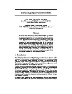
Submerged Kelp Detection with Hyperspectral Data Florian Uhl 1, *, Inka Bartsch 2 and Natascha Oppelt 1 1 2
*
Department of Geography, Kiel University, Ludewig-Meyn-Str. 14, Kiel 24118, Germany;
[email protected] Alfred-Wegener-Institute, Helmholtz Centre for Polar and Marine Research, Am Handelshafen 12, Bremerhaven 27570, Germany;
[email protected] Correspondence:
[email protected]; Tel.: +49-431-880-5583
Academic Editors: Deepak R. Mishra, Richard W. Gould and Prasad S. Thenkabail Received: 31 March 2016; Accepted: 2 June 2016; Published: 8 June 2016
Abstract: Submerged marine forests of macroalgae known as kelp are one of the key structures for coastal ecosystems worldwide. These communities are responding to climate driven habitat changes and are therefore appropriate indicators of ecosystem status and health. Hyperspectral remote sensing provides a tool for a spatial kelp habitat mapping. The difficulty in optical kelp mapping is the retrieval of a significant kelp signal through the water column. Detecting submerged kelp habitats is challenging, in particular in turbid coastal waters. We developed a fully automated simple feature detection processor to detect the presence of kelp in submerged habitats. We compared the performance of this new approach to a common maximum likelihood classification using hyperspectral AisaEAGLE data from the subtidal zones of Helgoland, Germany. The classification results of 13 flight stripes were validated with transect diving mappings. The feature detection showed a higher accuracy till a depth of 6 m (overall accuracy = 80.18%) than the accuracy of a maximum likelihood classification (overall accuracy = 57.66%). The feature detection processor turned out as a time-effective approach to assess and monitor submerged kelp at the limit of water visibility depth. Keywords: macroalgae; AISA; Helgoland
hyperspectral;
coastal;
airborne;
kelp;
imaging spectroscopy;
1. Introduction Kelp ecosystems dominate approximately 25% of the world’s rocky shores [1]. Kelps belong to the brown algae of the order Laminariales and form submerged forests of macroalgae. They are one of the key structures in worldwide coastal ecosystems and of great importance for ecosystem functions, aquaculture and food industries [2,3]. Kelp is relevant in determining patterns of abundance and food supply for fish and invertebrates [4]. Its occurrence is strongly related to the resources required by different life history stages of fish populations, providing foraging habitat and spatial refuge from predators [5]. Kelp also has a growing economic value and is harvested for human food consumption as well as being used in the alginate, mannitol and iodine industry [6,7]. The high biological productivity, fast growth and high polysaccharide content make macroalgae and, therefore, also kelp forests attractive for biofuel production [8]. Thus, these harvested patterns and human uses can affect coastal ecosystems and economies. Kelp is a sessile life form and constitutes persistent mats or three-dimensional forests in the coastal eutrophic subtidal zones. The forests flourish from the low tide level up to a depth of 20–30 m, depending on the turbidity of coastal zones [9]. The species vary considerably in form and size. In the N-Atlantic kelp species often grow to about 2–3 m in length [10] and forests have to be tolerant to the physical conditions of their environment, i.e., diurnal or seasonal variations in temperature, salinity,
Remote Sens. 2016, 8, 487; doi:10.3390/rs8060487
www.mdpi.com/journal/remotesensing
Remote Sens. 2016, 8, 487
2 of 20
water movement, nutrient and carbon delivery, light availability and levels of UV radiation [11]. Kelps are rather stenothermal and adapted to a narrow range of environmental conditions [12]. Thus, changes in the occurrence of kelp indicate changing environmental and habitat conditions caused e.g., by increasing water temperatures or sea level rise [13]. Kelp ecosystems are responding to climate driven habitat changes all over the world (e.g., Japan: [14], Tasmania: [15], Norway: [16,17], Spain: [18]). In many temperate regions, kelp forests are retreating due to ocean warming and human pressure [19,20]. Several modelling studies forecast a poleward shift of benthic marine species [21–23]. Recent field evidence also suggests that Arctic kelp ecosystems are currently undergoing change. At one site in Spitsbergen the depth distribution of kelps was found to be becoming shallower and biomass has increased considerably [16]. Possible driving forces are strongly connected to climate change, e.g., the change of the underwater irradiance climate, a lack of ice-scouring in winter, the elongation of the open-water period and increased sedimentation [16]. These climate driven changes and the concomitant threats to the marine flora and fauna are considered by the European Marine Strategy Framework Directive. Programs of measures for the protection and management of the marine environment should be implemented considering scientific and technological developments [24]. Rocky shore communities are highly suitable for long-term ecological studies and appropriate indicators of ecosystem health [25]. Most studies, however, have been conducted in intertidal habitats that are easily accessible but strongly influenced by tides and waves [26]. Few studies monitor subtidal habitats with canopy-forming macroalgae such as kelp, mainly because they are difficult to sample [27]. Remote sensing methods gather areal information about these habitats with less cost intensive field data sampling. In recent years, techniques have been developed for benthic mapping in clear waters [28–32]. Some studies also achieved promising results for mapping marine bottom types in turbid waters, e.g., [33,34]. A poor penetration of light into the water column however was the major limitation factor. The difficulty in analysing submerged plants is that their spectral reflectance is usually very low because water strongly absorbs electromagnetic radiation in the optical spectral region [35,36]. Experimental studies have shown that the contribution of submerged aquatic vegetation (SAV) to the measured remote sensing signal decreases with increasing depth of the water column over the vegetation, resulting in a diminished spectral signal of the target species [37], whereas absolute reflectances of emergent macroalgae, like kelp and other brown algae, significantly increase with desiccation [38]. Further variability is introduced by changing water levels during tides and due to currents resulting in a mixing of plant and water signal [39]. Optically active water components, such as suspended solids or chlorophyll, may share spectral features with SAV [40]. The spectral signature of aquatic vegetation therefore shows overlapping signatures from water resulting in a wide range of reflectance values impeding classification [41]. Satellite-borne systems are particularly suitable for long-term monitoring due to their high temporal resolution. Several studies use multispectral satellite systems to achieve information about SAV (e.g., [42–44]), but remote sensing of benthic ecosystems can only make use of spectral bands in the wavelengths at approximately 400–740 nm which penetrate into the water [45]. The narrow bandwidths of forthcoming hyperspectral missions like EnMAP [46] or PRISMA [47] provide a better spectral resolution in the visible wavelength range. This enables the detection of local features for kelp and macroalgae detection in general [48]. Unfortunately, these systems are still unavailable and suitable approaches currently can only be developed using airborne hyperspectral systems. The airborne systems have already been shown to be suitable for mapping seagrass species, cover and biomass in clear shallow waters [49] and to differentiate between macroalgae and floating seagrass mats [50]. The development of new methods should therefore ensure transferability to satellite-borne systems. In the present study, we developed a fully automated simple processor to detect the presence of kelp from airborne hyperspectral AisaEAGLE data. The algorithm is designed to work without the need of field data or intense training. The approach consists of three steps: (1) an anomaly filter to
Remote Sens. 2016, 8, 487
3 of 20
Remote Sens. 2016, 8, 487
20 remove effects on the water surface; (2) a derivative-based algorithm for kelp-feature extraction3 of and (3) an identification of kelp dominated pixels using specific spectral features of kelps. The aim of this algorithm is to reduce the depth limitations imposed by reflectance-based classification methods. algorithm is to reduce the depth limitations imposed by reflectance-based classification methods. Therefore, we compare the results with a common maximum likelihood classification without Therefore, we compare the results with a common maximum likelihood classification without anomaly filtering. anomaly filtering.
2. 2. Materials Materialsand andMethods Methods 2.1. 2.1. Study Study Site Site The is is located 50 50 kmkm off off thethe German coastline in the The archipelago archipelago of ofHelgoland Helgoland(54°11′N, (54˝ 111 N,7°53′E) 7˝ 531 E) located German coastline in central German Bight (North Sea)Sea) (Figure 1a).1a). It is the only the central German Bight (North (Figure It is the onlyterrestrial terrestrialsite siteininthis thisregion region with with an an offshore sandstone offshore character character [51]. [51]. Helgoland Helgoland is is divided divided into into two two small small islands: islands: the the main main rocky rocky red red sandstone 2 2 island island Helgoland Helgoland with with an an areal areal coverage coverage of of 1.1 1.1 km km and and the the smaller smaller sandy sandy dune dune island island with with 0.6 0.6 km km22.. The subtidal zone zone around aroundthe thetwo twoislands islandsisisthe theonly onlyhard-bottom hard-bottomlocality locality south-eastern part The subtidal inin thethe south-eastern part of of the North Sea [52]. The region is characterized by an offshore climate with perennial rainfall the North Sea [52]. The region is characterized by an offshore climate with perennial rainfall (average (average annual precipitation 752 low mm)annual and low annual air temperature = annual precipitation = 752 mm)=and air temperature fluctuationsfluctuations (daily mean(daily = 9.8 ˝mean C) [53]. 9.8 °C) [53]. According to Franke et al., (2004) observed changes in the composition of subtidal According to Franke et al., (2004) observed changes in the composition of subtidal macroalgae macroalgae communities may indicate a climate shift from North Sea climate towards more oceanic communities may indicate a climate shift from North Sea climate towards more oceanic conditions conditions (higher mean winter water temperature, and more constant[54]. salinities) [54]. (higher mean winter water temperature, higher and higher more constant salinities)
Figure 1.1.(a)(a) TheThe location of Helgoland is outlined a map of Europe (data of source: openstreetmapdata. location of Helgoland is inoutlined in a map Europe (data source: com); (b) A bathymetric map based on sea chart zero astronomical tide) ofastronomical the subtidal openstreetmapdata.com); (b) A bathymetric maplevel based on (lowest sea chart level zero (lowest zone of (data courtesy of Federal Maritime andof Hydrographic Agency of tide) of the the archipelago subtidal zone of source: the archipelago (data source: courtesy Federal Maritime and Germany 2010). Hydrographic Agency of Germany 2010).
The the subtidal subtidal of of the the archipelago archipelago demarcated demarcated by the 20-metre 20-metre isobaths isobaths derived The study study site site is is the by the derived from a bathymetric map from the Federal Maritime and Hydrographic Agency of Germany from a bathymetric map from the Federal Maritime and Hydrographic Agency of Germany (Figure 1). (Figure 1). is This is to theestimate basis to estimate theofdepth of the detected kelp patches this study. The This map themap basis the depth the detected kelp patches in thisin study. The map map has depth five depth classes between 0 and 20 m: 2–5m;m;5–10 5–10mmand and10–20 10–20m. m. We has five classes between 0 and 20 m: >0 >0 m;m; 0–20–2 m;m; 2–5 We also also interpolated (Figure 1b). 1b). The interpolated these these classes classes to to achieve achieve aa second second infinitely infinitely variable variable depth depth map map (Figure The bottom bottom substrates substrates along along Helgoland’s Helgoland’s shore shore are are red red sandstone, sandstone, chalk chalk and and flint flint stone. stone. The The rocky rocky seafloor seafloor forms forms an eroded terrace north and west of the main island. Significant beach nourishments in the early twentieth century moulded the natural rock base south and east of the main island. Nevertheless, the characteristic morphology of the rocky substratum still offers numerous small habitats as an ideal environment for highly diverse macroalgae communities [55]. Extensive kelp forests of the brown
Remote Sens. 2016, 8, 487
4 of 20
an eroded terrace north and west of the main island. Significant beach nourishments in the early twentieth century moulded the natural rock base south and east of the main island. Nevertheless, the characteristic morphology of the rocky substratum still offers numerous small habitats as an ideal environment for highly diverse macroalgae communities [55]. Extensive kelp forests of the brown algae species Laminaria digitata, Laminaria hyperborea, Saccharina latissima and Desmarestia aculeata dominate the subtidal zone. They are accompanied by an understorey of red algae, e.g., Delesseria sanguinea, Plocamium cartilagineum or Polysiphonia sp. The solid substrates in the subtidal are nearly always covered by algae [56]. Brown algae of the species Fucus serratus form dense canopies on the intertidal sandstone ridges, but their occurrence ends at the infralittoral zone [57]. The high turbidity of the waters around Helgoland limits the lower growth limit of Laminariales at about 8–10 m, whereas red-algae still occur in depths up to 20 m [9,56]. 2.2. Field Survey Mapping via diving transects is a well-established method to investigate subtidal zones [56,58]. For this study, we used georeferenced transect diving mappings conducted during two intensive field campaigns in summer 2010 and 2011 (Figure 2) which serve as reference for our remote sensing study. As the subtidal kelp forest is mostly built up by the perennial kelp Laminaria hyperborea [56,58], there is considerable stability over time in the presence of the forest [56,59]. Thus, the diving information of both years was used here as validation reference for the remote sensing study. Data were collected at regular intervals along a horizontal line at the sea floor and species presence/absence and abundances were recorded. The divers recorded the algal cover approximately every six meters. The distance was measured with the help of a 2 m stick. The precision of this underwater distance measurement is not comparable with land measurements and is influenced by drift and water movement. Therefore, the distance of the recorded points generally varied between 5 m and 10 m but was sometimes even bigger explaining the partially observable gaps in the diving ground truth information (Figure 2). Geo-referencing was achieved in the following way: the divers carried a buoy with an attached Magellan GPS 320 receiver to achieve point location information for their measurements. At regular distances, the line holding the buoy was pulled straight above the head of the diver and later the subtidal position was correlated via the synced time stamps of the GPS and the diving computer. Figure 2 illustrates the spatial distribution of transects in the study area. Measurements were conducted every six metres (mapping radius three metres) and included: 1. 2.
Cover estimation of the four dominant brown macroalgae (Laminaria digitata, Laminaria hyperborea, Saccharina latissima, Desmarestia aculeata). Presence/absence of brown algae Water depth measurement using a digital depth gauge (Seemann Sub; precision: 40 cm) and transferred to sea chart level zero [56].
A detailed description of the diving data acquisition is published by Pehlke and Bartsch (2008) [56]. Altogether, the divers mapped 21 transects during the two campaigns. The mapped data were transferred into a Geographical Information System (GIS). The depth measures were converted to sea chart level zero with help of the tide gauge level data Helgoland [60]. Coinciding with the mappings we documented the status of the main kelp habitats with photographs. The diving mappings only capture the subtidal areas of the study area. We used intertidal field mappings in addition to the diving data for the validation of the remote sensing classifications results in shallow waters [41,61]. The intertidal areas are mainly dominated by brown algae from the order Fucales. These mappings in combination with digital orthophotos enable an evaluation of whether the classification methods successfully separate kelp habitats from Fucales habitats in the shallow waters of the study area.
Mapping via diving transects is a well-established method to investigate subtidal zones [56,58]. For this study, we used georeferenced transect diving mappings conducted during two intensive field campaigns in summer 2010 and 2011 (Figure 2) which serve as reference for our remote sensing study. As the subtidal kelp forest is mostly built up by the perennial kelp Laminaria hyperborea [56,58], there is considerable stability over time in the presence of the forest [56,59]. Thus, the diving information of Remote Sens. 2016, 8, 487 5 of 20 both years was used here as validation reference for the remote sensing study.
Figure Figure 2. 2. Overview Overview of of diving diving transects transects (a–h), (a–h), flight flight stripe stripe cover cover of of the the study study area area (i) (i) and and overview overview of of diving transects (j–o); the colouring indicates the percentage cover of kelp mapped by the divers. diving transects (j–o);
2.3. Hyperspectral Data The remote sensing data of the study site was acquired using a hyperspectral AisaEAGLE system. The progressive scan CCD detector system consists of a high efficiency transmissive imaging spectrograph, a diffuse down welling irradiance collector (FODIS), an Oxford RT3100 global positioning system (GPS), inertial measurement unit (IMU) (position accuracy ě 1.8 m) and a computer for data storage and system control [62,63]. The radiometric resolution of the spectrograph is 12 bit for up to 488 spectral bands within a spectral range of 400–900 nm and with a spectral sampling rate of 3.3 nm. To gain a better signal to noise ratio the sensor was set to a spectral binning of four resulting in 120 spectral bands with a sampling rate of 4.6 nm. Furthermore, a spatial binning of two produced 512 pixels across track. Altogether, thirteen flight stripes were recorded on 9 May 2008 (Figure A1) with a motor glider Condor Stemme S10 owned by Orbital High-technology Bremen (OHB System AG). Data acquisition took place between 10:00 and 11:45 h UTC at low tide under sunny and calm
Remote Sens. 2016, 8, 487
6 of 20
conditions at an altitude of 693 m (2300 ft) above sea level and a velocity of 31 m/s (112 km/h) (Table 1). The resulting pixel spacing is 0.92 m along track and 0.68 m across track. Table 1. Flight stripe (FS) acquisition time of day (UTC). FS Start time
1
2
3
4
5
6
7
8
9
10
11
12
13
10:08 10:20 10:27 10:34 10:41 10:48 10:53 10:59 11:05 11:19 11:27 11:36 11:42
The AISA data were radiometrically pre-processed and calibrated using the software CaliGeoPro [62]. Geometric correction was conducted using the GPS/IMU data acquired during the flight and boresight calibration measurements. The pixels were afterwards resampled to 1 ˆ 1 m pixel spacing using the nearest neighbour approach. The radiometric pre-processing included a dark current correction and a sensor calibration using data provided by SPECIM. At-Sensor reflectances were obtained using the FODIS measurements. The next step of data processing was an atmospheric correction to surface reflectance using ATCOR-4 [64]. Tec5 HandySpec [65] (spectral range 350–950 nm, spectral sampling interval 3 nm) field spectrometer data collected during the AISA data acquisition were used to validate the AISA reflectance values. We further masked land and emergent surfaces using a reflectance threshold at 957 nm and further flagged pixels with a reflectance higher than 3% and 10%, respectively. The WAF algorithm is written with the programming language IDL for the software EnMAP-Box [66]. 2.4. Kelp Detection We developed and applied a fully automatic processor to detect the presence or absence of kelp in remote sensing images of subtidal rocky coastal shores. The program is divided into two steps: at first a Water Anomaly Filter (WAF) is applied to prepare the data for the kelp analysis and, secondly, a spectral kelp feature detection was used to separate kelp pixels from non-kelp pixels. 2.4.1. Water Anomaly Filter—WAF WAF is a spatial function to remove and replace outliers (spectral anomalies) that negatively influence the kelp detection algorithm. We define anomalies as single pixels with exceptionally high reflectance values compared to the relatively low water spectra, i.e., pixels with a high spatial frequency. This includes sunglint, foam or small anthropogenic objects (e.g., buoys, boats). Due to different emergent radiant flux from the water and varying offsets from the surface and path radiances, the signal from affected water pixels may be the same as the signal from unaffected ones. The detection and correction of anomalies therefore cannot be performed with constant (global) parameterisation and single pixel calculations without considering neighbouring regions. Using an anomaly filter we analysed the surrounding of each pixel (x) to detect whether it is an anomaly or not. WAF is based on a moving window approach and works in four steps: (1) A spatially adaptive filter with a kernel size of (i = 5) ˆ (j = 5) is applied; (2) WAF calculates the arithmetic mean (x) (Equation (1)) and the standard deviation (σ) (Equation (2)) of the moving window excluding the centre pixel (x3,3 ) as well as pixels with zero values. The centre pixel is excluded from the mean calculation emphasizing that kelp forest has a large spatial extent in contrast to small-scale water surface anomalies. ˛˛ ˛ ¨¨ ¨ 5 5 1 ˝˝ ÿ ˝ ÿ ` ˘‚‚ xi,j ´ x3,3 ‚ x“ 24
(1)
¨¨ ¨ ˛˛ ˛ 5 5 ˘ 1 ˝˝ ÿ ˝ ÿ ` σ“ xi,j ´ x ‚‚´ px3,3 ´ xq‚ 24
(2)
i“1
i“1
j“1
j “1
Remote Sens. 2016, 8, 487
7 of 20
(3) The outlier corrected arithmetic mean (xoc ) is calculated again, including all pixels within the range of the standard deviation (noc ). The result is an outlier corrected mean value (Equation (3)). ¨ xoc “
1 ˝ noc
5 ÿ
i“1
¨
5 ÿ
˝ j “1
#
˛˛ xi,j , if px ´ σq ď xi,j ď px ` σq and pi ‰ 3 and j ‰ 3q ‚‚ 0, else
(3)
(4) In a final step, we check whether the central pixel value is within the standard deviation of the outlier corrected mean value. If this condition is met, the central pixel keeps its original value; otherwise, the value is replaced by the new arithmetic mean (Equation (4)). # x3,3 “
x3,3 , if pxoc ´ σq ď x3,3 ď pxoc ` σq xoc , else
(4)
The kernel passes along each row of pixels (ignoring the edge pixels) producing a new image. 2.4.2. Feature Detection—FD The Feature Detection is a three-step classification algorithm to separate kelp-dominated pixels from non-kelp pixels. Uhl et al., 2013 [67] already showed how to use derivative feature detection for macroalgae analysis. First, the algorithm calculates the first order derivative for each pixel. Derivatives of the first order provide information about the rate of change in the reflectance of neighbouring bands. This enables the identification of local minimum and maximum values (spectral features), reduces spectral noise and separates overlapping features in the spectral signatures of water, sediment and kelp [38,68,69]. Spectral noise generally has a high impact on the quality of derivatives [70]. To smooth the spectra we therefore applied the digital polynomial Savitzky–Golay filter [71]. The first derivative R1 pλb q on wavelength λb from band number b was calculated using a seven band range (three bands on either side of the central band) and a polynomial degree of two. In the second step, we looked for zero transition points λ f in the first derivative spectrum. If the sign of the derivative between two successive bands changed, we determined the wavelength location of this feature (Equation (5)). The wavelength locations of all features of each single spectrum were stored as a feature location list. $ ` ˘ λ ´λ ’ λb ` R1 λ b`1 ´Rb1 λ , i f R1 pλb q ą 0 and R1 pλb`1 q ă 0 ’ ’ p b q| | p b`1 q ’ & λf “ ` ˘ ’ ’ or R1 pλb q ă 0 and R1 pλb`1 q ą0 ’ ’ % ND, else
(5)
In a last step, the algorithm analysed the feature list of each spectrum for specific features. If a spectrum showed all specified features, it was identified as a kelp-dominated pixel. In a previous study, Uhl et al., 2013 [67] used laboratory and remote sensing reflectance spectra of kelp to identify the feature wavelengths, i.e., spectral ranges with features significant for kelp detection. They reported suitable spectral regions in the wavelength range of 500–712 nm. However, we had to check whether these features were still apparent with submerged kelp. For this reason, we performed a spectral analysis to identify depth invariant kelp features (Section 3.1). Finally, the algorithm classifies a pixel as (dominated by) kelp if it shows features in all selected wavelength ranges. The FD algorithm was written with the programming language IDL for the software EnMAP-Box [66]. FD and WAF codes are available as supplementary data for this paper. 2.5. Maximum Likelihood Classifier—MLC Maximum likelihood classification (MLC) is a well-established supervised classification method and has often been applied for the mapping of brown algae e.g., [72,73]. MLC quantitatively evaluates the variance and covariance of the spectral pattern in each class to classify an unknown pixel. Assuming
Remote Sens. 2016, 8, 487
8 of 20
a normal distribution, mean vector and covariance matrix describe the spectral patterns of each class. Using the probability density function, the probability of a pixel can be calculated for each class. Each pixel will be assigned to the most likely class or be labelled unclassified if the probability value is below a user-defined threshold [74]. In this study, we used the software ENVI 4.8 (Exelis Visual Information Solutions, Boulder, CO, USA) to run the MLC. We analysed photographs and digital orthophotos to set the training plots for the two classes (kelp and non-kelp). To ensure comparability with the FD algorithm, the MLC was not performed with depth-dependent zonal classes as proposed by other studies [75,76]. Furthermore, such an approach would imply more extensive field data collection. Each training class had at least 3000 pixels for the training of the classifier. The spectral range of the input data was reduced to the visible region (402 nm–696 nm) obtaining 65 spectral bands and the probability threshold was set to 0.05. 2.6. Validation of Classification Results The spatial resolution of the AisaEAGLE data is higher than the transect mappings with an approximate radius of three metres around each mapping point (Figure 3); on average, 38 pixels cover Remote Sens. 2016, 8, 487 8 of 20 the same area as a single diving mapping point. After FD and MLC classification, we adjusted the remote data the spatial of theAfter diving examinedwe theadjusted accuracy thesensing same area as to a single divingresolution mapping point. FDmapping and MLCand classification, theof the classification results with two methods. For the first statistical analysis, we calculate the percentage remote sensing data to the spatial resolution of the diving mapping and examined the accuracy of coverthe from the AISA classifications by counting and dividing themwe bycalculate the total the number classification results with two methods. all Forkelp the pixels first statistical analysis, percentage from the classifications all kelp pixels and dividing them by the kelp of pixels withincover the range of AISA a mapping point. by Wecounting then compare this measure to the mapped of pixelstransect within the range of point a mapping point. WeThis then method compare is this measure to the the covertotal for number the respective mapping (Figure 3a). used to validate mapped kelp cover for the respective transect mapping point (Figure 3a). This method is used to For results from each single flight stripe and to exclude unsuitable flight stripes from further analysis. validate the results from each single flight stripe and to exclude unsuitable flight stripes from further each flight stripe we calculate three accuracy measures, i.e., root-mean-square error (RMSE), Pearson analysis. For each flight stripe we calculate three accuracy measures, i.e., root-mean-square error product-moment correlation coefficient (R2 ) and Nash–Sutcliffe model efficiency coefficient (NSE) [77]. (RMSE), Pearson product-moment correlation coefficient (R2) and Nash–Sutcliffe model efficiency We use the setup of three different measures to confirm the accuracies with different accuracies: the coefficient (NSE) [77]. We use the setup of three different measures to confirm the accuracies with RMSE is the average percentage between the diving mapping and kelpmapping detection results; different accuracies: the RMSEdeviation is the average percentage deviation between thethe diving and 2 R is the a measure for a linear correlation between datasets andbetween NSE assesses the overall match of kelp detection results; R2 is a measure for aboth linear correlation both datasets and NSE mapped and the remotely data. NSE = 0 indicates an accuracy as good as the mean of the mapped assesses overallsensed match of mapped and remotely sensed data. NSE = 0 indicates an accuracy as as close the mean of refer the mapped data, values close toand +1 refer to anvalues accurate detection and negative data,good values to +1 to an accurate detection negative indicate that the accuracy is that worse than the mean of the mapped data. worsevalues than indicate the mean ofthe theaccuracy mappedis data.
Figure 3. Validation of the FeatureDetection Detection (FD) (FD) and Likelihood Classification (MLC) Figure 3. Validation of the Feature andMaximum Maximum Likelihood Classification (MLC) results using a single diving transect mapping point: (a) percentage coverage comparison and results using a single diving transect mapping point: (a) percentage coverage comparison and (b) kelp/non-kelp detection. (b) kelp/non-kelp detection.
The second statistical analysis evaluates the feasibility of FD and MLC to distinguish kelp-dominated and non-kelp areas (Figure 3b). An area is marked as kelp dominated, if 50% or more of the pixels within the reach of a validation point detect kelp. We also adjust the diving transects mapping to this differentiation, i.e., a mapping point result indicating >50% coverage of brown algae is flagged as presence of kelp. Prior to the second analysis, a subset of suitable flight stripes
Remote Sens. 2016, 8, 487
9 of 20
The second statistical analysis evaluates the feasibility of FD and MLC to distinguish kelp-dominated and non-kelp areas (Figure 3b). An area is marked as kelp dominated, if 50% or more of the pixels within the reach of a validation point detect kelp. We also adjust the diving transects mapping to this differentiation, i.e., a mapping point result indicating >50% coverage of brown algae is flagged as presence of kelp. Prior to the second analysis, a subset of suitable flight stripes determined by the first analysis is merged to single image. Accuracy measures are the overall accuracy, error of omission and error of commission [78]. 3. Results and Discussion 3.1. Wavelength Range for Deep Kelp Detection The photochemical properties of kelp mainly influence the spectral reflectance in the visible part of the electromagnetic spectrum. For SAV, the spectral properties of water influence these spectral Remote Sens. 2016, 8,The 487 location of spectral features shifts with varying water level or features may 9even of 20 characteristics. disappear. The behaviour of kelp spectra under varying water column is the basis to determine the wavelength intervals intervals of of the the FD FD algorithm wavelength algorithm because because the the FD FD algorithm algorithm requires requires unique unique local local reflectance reflectance minima or maxima. To determine suitable wavelength intervals, we extracted kelp spectra the minima or maxima. To determine suitable wavelength intervals, we extracted kelp spectra from from the AisaEAGLE data data at at different different depth depth levels. levels. Figure sequence of of AISA AISA Laminaria Laminaria spectra spectra AisaEAGLE Figure 44 shows shows aa sequence achieved from different depth positions (Figure 4b–e) derived from the bathymetric map depth achieved from different depth positions (Figure 4b–e) derived from the bathymetric map depth classes classes in comparison a dry kelp laboratory spectrum (Figure The characteristic absorption in comparison to a dryto kelp laboratory spectrum (Figure 4a) [38]. 4a) The[38]. characteristic absorption troughs troughs of the main pigments fucoxanthin, chlorophyll c and chlorophyll a are highlighted for each of the main pigments fucoxanthin, chlorophyll c and chlorophyll a are highlighted for each spectrum. spectrum. The absorption features from allare pigments visible in the laboratory spectrum The absorption features from all pigments visible are in the laboratory spectrum (Figure 4a)(Figure as well4a) as as well as in the AISA spectrum (Figure 4b). A water depth of 0–2 m results in a less distinctive in the AISA spectrum (Figure 4b). A water depth of 0–2 m results in a less distinctive chlorophyll c chlorophylland c absorption and the disappearance of spectral 585nm nm(Figure and 6304c). nm (Figure 4c). absorption the disappearance of spectral troughs at 585troughs nm andat630
4. Savitzky-Golay Figure 4. Savitzky-Golay smoothed smoothed kelp kelp (Laminaria (Laminaria digitata) digitata) laboratory laboratory measurements measurements (a) and Savitzky-Golay ROI AISA kelp (Laminaria hyperborea) hyperborea) spectra spectra with with varying varying water water cover cover (b–e). (b–e).
Increasing water also affects other spectral features (Figure(Figure 4d). A reflectance peak at 570peak nm Increasing waterdepth depth also affects other spectral features 4d). A reflectance and troughs at troughs 527 nm and 675nm nmand are 675 the only local maxima/minima still detectablestill at 2–5 m. At a at 570 nm and at 527 nm are the only local maxima/minima detectable depth of 5–10 m (Figure 4e), the water absorbs electromagnetic radiation >680 nm; the chlorophyll at 2–5 m. At a depth of 5–10 m (Figure 4e), the water absorbs electromagnetic radiation >680 nm; the absorption at 675 nm therefore ReflectanceReflectance between 450 and 570 higher chlorophyll absorption at 675 nmbecomes thereforeundetectable. becomes undetectable. between 450nm andis570 nm compared to the shallower algae spectra duespectra to additional ofreflection the turbidof waters. The spectral is higher compared to the shallower algae due toreflection additional the turbid waters. analysis reveals only two spectral of kelpfeatures for all depth levels. first islevels. the wavelength The spectral analysis reveals onlyfeatures two spectral of kelp for The all depth The first range is the of 510–546 nm mainly influenced by fucoxanthin absorption, whereas this absorption feature shifts from shorter wavelengths (low water influence, Figure 4b) to longer wavelengths (deeper areas, Figure 4e). The second feature is a reflectance peak between 560 and 580 nm. The results clearly show that the wavelength region >600 nm is unsuitable to detect spectral features of submerged kelp. In the turbid waters around Helgoland, longer wavelengths are only feasible for the detection of
Remote Sens. 2016, 8, 487
10 of 20
wavelength range of 510–546 nm mainly influenced by fucoxanthin absorption, whereas this absorption feature shifts from shorter wavelengths (low water influence, Figure 4b) to longer wavelengths (deeper areas, Figure 4e). The second feature is a reflectance peak between 560 and 580 nm. The results clearly show that the wavelength region >600 nm is unsuitable to detect spectral features of submerged kelp. In the turbid waters around Helgoland, longer wavelengths are only feasible for the detection of shallow, emergent or floating algae. To detect kelp in different water depths, it is necessary to use the spectral range between 500 and 600 nm, where two suitable spectral features are located at 528 nm ˘ 18 nm and at 570 nm ˘10 nm. 3.2. WAF Performance Water anomalies have a strong influence on the results of the feature detection algorithm. Initial tests of feature detection without prior filtering resulted in erroneous kelp detection at sites influenced by sun glint. By removing outliers WAF significantly improves the FD results. Figure 5 shows some examples of WAF performance. The imagery is strongly influenced by sunglint before data correction Remote Sens. 2016, 8, 487 10 of 20 (Figure 5a,c) while sun glint is significantly reduced by filtering (Figure 5b,d).
Figure water anomaly filtering (WAF(WAF performance) on imagery quality atquality sites influenced Figure 5.5.Influence Influenceof of water anomaly filtering performance) on imagery at sites by sun glint. True colour RGB (639 nm/550 nm/459 nm) for two example areas. Area 1 influenced by sun glint. True colour RGB (639 nm/550 nm/459 nm) for two examplebefore areas.filtering Area 1 (a) andfiltering after filtering (b)after andfiltering area 2 before filtering and filtering after filtering (d). before (a) and (b) and area 2 (c) before (c) and after filtering (d).
WAF performance may also be an indicator of data quality, because the amount of corrected pixels indicates image homogeneity. Table 2 shows the percentage of WAF corrected pixels for every flight stripe. Table 2. Pixels changed by the WAF Table WAF in in percent percent (%) (%) of of all all pixels pixels Flight Stripe 1 Flight Stripe corrected pixels (%) 2.91 corrected pixels (%)
2 3.89
3 4 5 3 4 5 2.24 2.11 3.06
1
2
2.91
3.89
2.24
2.11
3.06
6 6 4.15
4.15
7 7 11.65 11.65
8 9 10 9 10 11 11.88 5.51 4.42
8
11.88
5.51
4.42
4.17
11 12 4.17
4.92
12 13 4.92 6.56
13 6.56
The data depict an increasing percentage of corrected pixels with increasing flight stripe. The data increasing corrected pixels with increasing flight stripe. Moreover, Moreover, thedepict flightanstripes eightpercentage and nine of show exceptionally high numbers of corrected pixels. the flight stripesreveals eight and nine show exceptionally high numbers pixels. VisualThe analysis Visual analysis an increase of sunglint from flight stripe oneoftocorrected flight stripe thirteen. flight reveals an increase of sunglint from flight stripe one to flight stripe thirteen. The flight stripe numbers stripe numbers correspond with the time of day during image acquisition (Table 1), whereas azimuth correspond withremains the timeconstant of day during image acquisition (Table7,1), whereas azimuth sun flight direction flight direction for most of the stripes except 8 and 13. Azimuth movement remains for sun-sensor most of thegeometries stripes except 7, 8 andthe 13.main Azimuth movementsunglint. resultingThe in resultingconstant in changing is therefore reasonsun for increasing changing sun-sensor geometries is therefore the main reason for increasing sunglint. The flight flight parameters from stripes seven, eight and thirteen corroborate this hypothesis. The flight parameters stripes seven, thirteen hypothesis. Thethe flight direction is direction is from approximately fromeight westand to east withcorroborate sun comingthis from south, while other data has approximately west to east sun coming south, while the stripes, other data has is been been recorded from in south-east to with north-west flightfrom direction. In these WAF notrecorded able to in south-east to north-west flight direction. In these WAF isareas not able sufficiently correct sufficiently correct the sunglint-artefacts, because thestripes, glint covered are to much larger than the the thefeature glint covered areas are muchdata larger than thepoorly. filter kernel size filtersunglint-artefacts, kernel size of 5 × 5because pixels. For detection, non-filtered performed of 5 ˆ 5 pixels. For feature detection, non-filtered data performed poorly. 3.3. Kelp Detection Results Validated with Diving Transects Interpreting kelp detection results visually, feature detection successfully captures the kelp forests in the deep waters around Helgoland. The approach identifies kelp on the rocky ridges and excludes sandy channels (Figure 6). Reflectance signal from the rocky bottom substrates did not influence the kelp detection results. Macroalgae completely cover the solid substrates in the intertidal. The reflected signal from these areas is therefore mainly influenced by the water column and macroalgae. Kelp does not grow on unconsolidated substrates. Spectral mixing between the sandy
Remote Sens. 2016, 8, 487
11 of 20
3.3. Kelp Detection Results Validated with Diving Transects Interpreting kelp detection results visually, feature detection successfully captures the kelp forests in the deep waters around Helgoland. The approach identifies kelp on the rocky ridges and excludes sandy channels (Figure 6). Reflectance signal from the rocky bottom substrates did not influence the Remotedetection Sens. 2016, results. 8, 487 11 of 20 kelp Macroalgae completely cover the solid substrates in the intertidal. The reflected signal from these areas is therefore mainly influenced by the water column and macroalgae. Kelp does for classification validation (Figure 7). We first verified whether the the sandy featureridges detection successfully not grow on unconsolidated substrates. Spectral mixing between and kelp is not a estimates percentage coverage of kelp. Table 3 shows the validation results for the FD using the major problem for this study area. Only the small edges between the two habitats suffer from spectral diving data. mixing. Therefore, both covers could clearly be separated by the kelp detection.
Figure 6. 6. (a) (a) Stretched Stretched true true colour colour image image of of selected selected flight Figure flight stripes stripes and and (b) (b) kelp kelp detected detected by by FD. FD.
Analysis of the of diving and theresults bathymetric shows that per theflight maximum depth Table 3. Validation the FDdata kelp detection with divemap transect mappings stripe (FS). for hyperspectral kelp detection around Helgoland is approximately six metres. Secchi depth FS 1 2 3 4 5 6 7 8 9 10 11 12 13 measurements on 9 May 2008 from the Helgoland Reede time-series reveal 4.1 m visibility depth [79]. RMSE 40.45 42.61 36.28 41.27 17.65 18.54 46.85 45.27 69.83 59.11 62.58 57.32 57.14 We assumed that the Secchi depth may be the limit for optical kelp detection; however, FD exceeds R2 0.43 0.43 0.40 0.38 0.70 0.72 0.39 0.33 0.06 0.16 0.20 0.29 0.03 the expectations by two metres. This difference may be explained by the growth form of kelp, which NSE −1.42 −1.28 −1.02 −0.93 0.57 0.65 −0.81 −0.94 −4.90 −2.05 −2.29 −1.93 −1.25 stands semi-erect in the water column, whereas the bathymetric map gives the depth to the sea floor. Thus, the path of the light can be shorter to the canopy of the kelp than to the sea floor. The divers also Validation with the transect mapping shows poor results, except flight stripe five and six which mapped kelp deeper than six metres, but these areas are not detected by the feature detection in the show RMSE lower than 20%, R2 greater or equal to 0.7 and NSE at approximately 0.6. Results from study area. We therefore reduced the diving mapping data to the depth range of zero to six metres the percentage kelp cover estimation showed poor results, indicating that FD might not be suitable for classification validation (Figure 7). We first verified whether the feature detection successfully to measure kelp coverage. Nevertheless, the calculated low accuracies do not match the good visual estimates percentage coverage of kelp. Table 3 shows the validation results for the FD using the interpretation results from Figure 6 and comparison with digital orthophotos and field photography diving data. showed good conformity with the FD results. We attribute the low accuracies to several factors. The low Table position accuracyofof diving transects (±25 is transect a substantial problem. buoy 3. Validation thethe FD kelp detection results withm) dive mappings per flightThe stripe (FS). GPS measurement induced an inaccuracy of several metres in the diving data as measurements were FS 1 2corrected 3 5 6 7 8 9 10buoy and 11 12 position, 13 non-differentially and4there always was a misalignment between diver RMSE 40.45 42.61 36.28 41.27 17.65 18.54 46.85 45.27 69.83 59.11 62.58 57.32 57.14 which tend to float and therefore constantly change their positions and field of view towards the 0.43 0.43 0.40 0.38 0.70 0.72 0.39 0.33 0.06 0.16 0.20 0.29 0.03 R2 measurement the AisaEAGLE have a´0.94 high spatial of 1 ×´1.93 1 m contrary NSE ´1.42 points. ´1.28 However, ´1.02 ´0.93 0.57 0.65 data´0.81 ´4.90 resolution ´2.05 ´2.29 ´1.25 to the spatial inaccuracy of the in situ measurements. This mismatch between imagery and ground truth data induces a failure in the correlation between percentage cover estimation by the divers and the hyperspectral imagery. The time-lag of two to three years between field mapping and remote sensing data acquisition may also have induced an error. Furthermore, classification errors primarily occur at pixels with insufficient sunglint removal. Conventional sunglint removal methods may be
highly inaccurate pixel locations (validated visually with digital orthophotos and other flight stripes). We therefore also excluded this stripe from further investigation. The second statistical analysis evaluates the feasibility of the feature detection to distinguish kelp-dominated and non-kelp pixels. Therefore, we merged the results of the kelp detection from all remaining flight stripes to a single image (Figure 7i) and did not calculate accuracy measures for each Remote Sens. 2016, 8, 487 12 of 20 single flight stripe.
Figure 7. Kelp detection detection validation validation results results with with diving diving transect transect mapping mapping (a–h), (a–h), cover cover of of the Figure 7. Kelp the selected selected flight stripes stripes (i) flight (i) and and kelp kelp detection detection validation validation results results (j). (j).
We compared of mapping the FD and mapping results achieving satisfactory The Validation withthe theresults transect shows poor results, except flight stripe fiveaccuracies. and six which overall accuracy of the kelp/non-kelp detection is 80.18%. 178NSE out of pixels of the0.6. diving mapping show RMSE lower than 20%, R2 greater or equal to 0.7 and at 222 approximately Results from match the remote sensing Of special interest the classification errors: the error the percentage kelp cover data. estimation showed poorare results, indicating that FD might notof beomission suitable is that FD was unable the to identify approximately 20% thematch kelp the mapped the to 18.92% measureindicating kelp coverage. Nevertheless, calculated low accuracies doofnot good by visual divers; with 0.90% thefrom errorFigure of commission indicates with that detected kelp pixels and are nearly always true interpretation results 6 and comparison digital orthophotos field photography kelp pixels. FDconformity therefore is with suitable absence or presence of kelp. showed good the for FDidentifying results. We attribute the low accuracies to several factors. The low position accuracy of the diving transects (˘25 m) is a substantial problem. The buoy GPS measurement induced an inaccuracy of several metres in the diving data as measurements were non-differentially corrected and there always was a misalignment between buoy and diver position, which tend to float and therefore constantly change their positions and field of view towards the measurement points. However, the AisaEAGLE data have a high spatial resolution of 1 ˆ 1 m contrary to the spatial inaccuracy of the in situ measurements. This mismatch between imagery and ground truth data induces a failure in the correlation between percentage cover estimation by the divers and the hyperspectral imagery. The time-lag of two to three years between field mapping and remote sensing data acquisition may also have induced an error. Furthermore, classification errors primarily occur at pixels with insufficient sunglint removal. Conventional sunglint removal methods may be suitable to reduce the sunglint and thus also the classification errors [80–82]. However, a first attempt
Remote Sens. 2016, 8, 487
13 of 20
to correct the sunglint with the method introduced by Kutser et al., (2009) showed unsatisfactory results. This is mainly addressed to the differing waterbodies around Helgoland. Flight stripes seven, eight and thirteen were therefore excluded from further analysis. Strong movements of the aircraft during recording of flight stripe nine caused errors in the geometric correction, which results in highly inaccurate pixel locations (validated visually with digital orthophotos and other flight stripes). We therefore also excluded this stripe from further investigation. The second statistical analysis evaluates the feasibility of the feature detection to distinguish kelp-dominated and non-kelp pixels. Therefore, we merged the results of the kelp detection from all remaining flight stripes to a single image (Figure 7i) and did not calculate accuracy measures for each single flight stripe. We compared the results of the FD and mapping results achieving satisfactory accuracies. The overall accuracy of the kelp/non-kelp detection is 80.18%. 178 out of 222 pixels of the diving mapping match the remote sensing data. Of special interest are the classification errors: the error of omission is 18.92% indicating that FD was unable to identify approximately 20% of the kelp mapped by the divers; with 0.90% the error of commission indicates that detected kelp pixels are nearly always true kelp pixels. FD therefore is suitable for identifying absence or presence of kelp. 3.4. Feature Detection Results Validated with Maximum Likelihood Classifier Spatial variations between the in situ data and the remote sensing data are one of the main reasons for lower accuracy measures of the kelp cover and presence/absence estimation. Therefore, in situ data alone seem to be insufficient to assess the suitability of the FD for kelp detection. We compared the FD to results with a commonly used MLC technique. This procedure enables an exact spatial comparability of the results. The flight stripes selected for this analysis capture the kelp forests around the main island and the area covered by them is shown in Figure 7i. We validated the MLC results comparable to the FD results (Section 3.3). Table 4 shows the accuracy measures of the MLC. Table 4. Validation of MLC results with dive transect mappings per flight stripe (FS). FS
1
2
3
4
5
6
10
11
12
RMSE R2 NSE
66.20 0.12 ´5.44
45.50 0.39 ´1.59
48.62 0.19 ´2.61
62.04 0.20 ´3.33
49.04 0.27 ´2.33
57.62 0.25 ´2.37
60.22 0.13 ´2.16
59.44 0.21 ´1.95
47.90 0.39 ´1.03
Compared to FD, MLC accuracies are significantly lower for all measures (RMSE Ø ´13.42; Ø ´0.17; NSE Ø ´1.46); except for flight stripes eleven and twelve. Nevertheless, the poor accuracies support the findings from Section 3.3, that georeferencing of diving mappings may be unsuitable to validate remote sensing data with high spatial resolution. For the second statistical measure, the kelp/non-kelp detection, we again merged the results of the MLC from the selected flight stripes to a single image. This analysis reveals an overall accuracy of 57.66% (n = 222), which is 22.52% lower than for the FD approach. The error of omission is 42.34% and the error of commission is zero. Thus, no areas have been falsely declared as kelp, but MLC was unable to identify several kelp areas (94 of 222 transect mapping points). The total cover of kelp detected by FD is 1.90 km2 while MLC detects 1.93 km2 . Although there is only a small difference in the total area of detected kelp between both classifications, detected areas are distributed unevenly. Figure 8a shows the spatial comparison of the two kelp detection results, visualizing that 80.45% of the kelp area matches for both methods, but MLC classifies 10.42% of kelp coverage mainly in very shallow waters close to the coastline, whereas FD detects 9.13% in waters deeper than 4 m. Table 5 shows the accuracies of FD and MLC for different depth limits using the diving depth gauge measures. R2
is only a small difference in the total area of detected kelp between both classifications, detected areas are distributed unevenly. Figure 8a shows the spatial comparison of the two kelp detection results, visualizing that 80.45% of the kelp area matches for both methods, but MLC classifies 10.42% of kelp coverage mainly in very shallow waters close to the coastline, whereas FD detects 9.13% in waters deeper than 4 8,m.487Table 5 shows the accuracies of FD and MLC for different depth limits using Remote Sens. 2016, 14 ofthe 20 diving depth gauge measures.
Figure 8. 8. Comparison Comparison of of FD FD and and MLC MLC kelp kelp detection detection results. results. (a) (a) Spatial Spatial distribution distribution of of the the classified classified Figure kelp and and (b) (b) kelp kelp area area detected detectedper perdepth. depth. kelp Table 5. Depth dependent kelp/Non-kelp detection accuracies. Depth Limit (m)
1
2
3
4
5
6
MLC overall accuracy (%) FD overall accuracy (%)
100 100
92.65 98.53
80.53 96.46
65.66 87.95
58.5 82
57.66 80.18
The overall accuracy of MLC drops significantly with a depth of four metres, while FD still sufficiently detects kelp at six metres depth (overall accuracy = 80.18). Figure 8b shows that the decreasing accuracy mainly results from kelp patches unidentified by MLC. The fully automatic FD detects kelp areas deeper than four metres with higher accuracy than the MLC. Both classifiers identify kelp between two and four metres water depth; due to the intensive training, however, MLC is much more labour-intensive. Nevertheless, differences between the two approaches are especially high in shallow waters (