Super-resolution Mapping via Multi-dictionary based Sparse ... - MIRLab

2014 IEEE International Conference on Acoustic, Speech and Signal Processing (ICASSP)

SUPER-RESOLUTION MAPPING VIA MULTI-DICTIONARY BASED SPARSE REPRESENTATION Huijuan Huang, Jing Yu, and Weidong Sun Department of Electronic Engineering, Tsinghua University ABSTRACT Based on the spatial dependence assumption, super-resolution mapping can predict the spatial location of land cover classes within mixed pixels. In this paper, we propose a novel super-resolution mapping method via multi-dictionary based sparse representation, which is robust to noise in both the learning and class allocation process. To better distinguish different classes, the distribution modes of different classes are learned separately. A spectral distortion constraint is introduced, combining with reconstruction errors as metrics to perform classification. The experiments prove that our method is superior to other related methods. Index Terms— Super-resolution mapping, spatial dependence, multi-dictionary learning, sparse representation 1. INTRODUCTION Multispectral and hyperspectral remote sensing images are commonly dominated by mixed pixels that contain more than one distinct substances due to imperfect imaging optics, secondary illumination, and the diverse distributed land cover classes. The mixed pixels decrease the classification accuracy dramatically. Atkinson [1] first introduced the concept of super-resolution mapping (SRM) based on the assumption of spatial dependence. This technique uses the fraction images yielded by spectral unmixing as input and can predict the spatial location of land cover classes within mixed pixels. SRM is also termed as subpixel mapping [2,3]. The current SRM methods can be roughly categorized into two groups [4]: spatial optimization types and learning-based types. In the first group, the spatial dependence is modeled by an objective function which is optimized to accomplish SRM [2, 3, 5, 6]. The difficulty is how to formulate mathematical models accurately and efficiently. The second group involves the Hopfield neural network method [7], geostatistical method [8], learning wavelets coefficients method [9], feed-forward back-propagation artificial neural network method [10], etc. The key issue with those methods is how to learn the prior information about distribution modes of land cover classes. Most of the neural network learning based SRM methods has the over-fitting problem, and they are also sensitive to noise in both the learning and class allocation process. Current methods usually interpret all class distributions following the same mode, which may not be applicable. For example, rivers usually distribute linearly, while islands distribute as oval areas. In this paper, land cover classes are treated discriminatorily by multiple dictionaries. There are many similar patches in natural images, and this type of ancillary information can be learned to form dictionaries by sThe work presented in this paper was supported in part by National Natural Science Foundation (61171117), National Science and Technology Pillar Program (2012BAH31B01), Key Project of the Science and Technology Development Program (kz201310028035) of China.

978-1-4799-2893-4/14/$31.00 ©2014 IEEE

3547

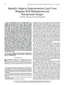
parse representation to do denoising [11], image restoration [12], face recognition [13], etc. Similarly, in land cover maps there exist repetitive distribution structures, such as linearly distributed rivers. Based on this assumption, we propose a new SRM method via multi-dictionary based sparse representation, referred to as MSRSM. In this paper, the proposed feature vector can capture the significant information about spatial dependence, and multiple distribution dictionaries are learned via sparse representation. In the class allocation process, the feature vector of the underlying subpixel is reconstructed by every dictionary, and is assigned to a class according to the reconstruction errors and the introduced spectrum distortions. Different land cover classes are interpreted separately in our framework, and this strategy leads to more accurate distribution dictionaries. It is worth noting that the sparse representation based learning is robust to noise, which has been demonstrated in the face recognition method [13]. The rest of the paper is organized as follows. Section 2 gives the SRM problem formulation. Section 3 presents the proposed MSRSM method in detail. The results of experiments are discussed in Section 4. Finally, the conclusion is drawn in Section 5 . 2. PROBLEM FORMULATION Super-resolution mapping technique uses the abundances yielded by spectral unmixing as inputs, and its output is a high-spatialresolution (HR) land cover map. Spectral unmixing the procedure by which the measured spectrum of a mixed pixel is decomposed into a collection of constituent spectra and proportions that indicate the abundances of each constituent present in the pixel. The theoretical basis of SRM is spatial dependence, which refers to the tendency that spatially proximate observation of a given property to be more alike than more distant observations. In the SRM strategy, coarse pixels with low spatial resolution (LR) are divided into several subpixels, and each subpixel is assigned to a proper class. Fig. 1 illustrates the principal of SRM intuitively. Fig. 1(a) is a window from fraction images, where the number indicates the percentage of the “Black” class occurring in the pixel. Based on the spatial dependence, the distribution mode in Fig. 1(c) is considered better than that in Fig. 1(b). Therefore, the key point to accomplish SRM is to find an efficient expression of spatial dependence either by an objective function or by learned prior knowledge. 3. THE PROPOSED METHOD The proposed MSRSM method mainly contains two steps: learning and SRM. In the learning step, using the HR training land cover maps, the training sample sets are first extracted, which can represent the spatial dependence effectively. Then the distribution dictionaries are learned via sparse representation. In the SRM step, the feature vector of the underlying subpixel is reconstructed by each distribution

(a)

(b)

(c)

Fig. 1: Explanation of the basic concept of SPM. (a) A window from fraction images, (b) One possible solution of SPM, (c) Better solution of SPM.

dictionary and the subpixel is assigned to a class with the principle of reconstruction errors and the introduced spectral distortion. Fig. 2 describes the framework of the proposed method.

(a)

(b)

Fig. 3: Illustration of the composition of the feature vector. (a) Description of symbols, (b) Calculation of the distance d.

The implication of sparsity is that when a signal has a sparse expansion, one can discard the small coefficients without much perceptual loss. Mathematically, suppose signal x ∈ Rn can be sparsely represented over an over-complete dictionary Φ ∈ Rn×m , m > n. Then x can be represented approximately as a linear combination of a few atoms from Φ , i.e., x = Φα, ∥α∥0 ≪ m , where ∥α∥0 means the number of nonzero entries of α . The solution of overcomplete dictionary Φ and sparse vector α can be formulated as the following optimization problem { } arg min ∥x − Φ α∥22 s.t. ∥α∥0 ≤ T (2)

Fig. 2: The framework of the proposed method.

Φ,α

3.1. The proposed feature vector Current learning based SRM methods usually use the abundances of a 3 × 3 neighborhood as the feature vector [9, 10], which is not effective enough to encode the spatial dependence. Let S represent the scale factor of spatial resolution, Pi,j denote the LR pixel at location (i, j), and each pixel is divided into S × S subpixels pka,b , with (a, b) being its location and k being its class label. All the symbols are depicted in Fig. 3(a). The proposed feature vector fk of pka,b is fk = [v1 , v2 , ..., vC ]T , where ]T [ c c Pi+1,j+1 Pi−1,j−1 ,..., (1) vc = d(pka,b , Pi−1,j−1 ) d(pka,b , Pi+1,j+1 ) d(pka,b , Pi−1,j−1 ) represents the distance between subpixel pka,b and c pixel Pi−1,j−1 , and Pi−1,j−1 , c = 1, . . . , C denotes the abundance of the cth class in pixel Pi−1,j−1 . That is to say, the feature vector is composed of the weighted abundance of all classes in the 3×3 neighborhood. Fig. 3(b) illustrates the calculation method of the weighted coefficients. It can be clearly seen that the pixel with greater abundance and nearer to the subpixel pka,b has greater weight, which means a larger impact on the subpixels class label. This demonstrates that the proposed feature can capture the significant information about spatial dependence. 3.2. Multi-dictionary based sparse representation Natural images can be sparsely represented by some certain dictionaries, such as DCT transform dictionaries, wavelet transform dictionaries, or learned dictionaries. Sparse representation has been widely used to learn this type of dictionary.

3548

where T is the sparsity threshold. In this paper, we learn the distribution dictionary for each land cover class via sparse representation. The kth training set for the kth land cover class is composed of the feature extracted from ∪ k vectors i the HR training images, i.e., Fk = n i=1 fk , with nk being the number of items in the set Fk . Then the kth distribution dictionary Dk is learned by

{ }

(3) arg min ∥Fk − Dk Ak ∥22 s.t. αki ≤ T Dk ,Ak

[

0

] k

where Ak = αk1 , . . . , αki , . . . , αt is the sparse coefficients matrix. We can solve the problem by alternating minimization of Dk by the K-SVD algorithm [14] and of Ak by the OMP algorithm [15]. 3.3. SRM based on the learned multi-dictionary During the SRM step, we use the proposed spectral distortion and reconstruction errors as metrics to perform classification. It is common to first determine the number of subpixels belonging to the kth class (denoted as Nk ). Subpixels are assigned only if the available subpixels for a particular class have not been completely exhausted. Current SRM methods usually set Nk = round(αk S 2 ), with the abundance αk constraint. This suggests that the accuracy heavily relies on that of the spectral unmixing algorithm, and usually leads to isolated pixels in the resulting land cover map. In this paper, we determine Nk by spectral distortion. This is inspired by the fact that in essence SRM discretizes the analogous abundances and inevitably contributes to some spectral distortion. Mathematically, it can be expressed as

2 C

∑

2 (4) Nk = arg min Nk sk /S − χ

Nk k=1

2

where sk is the spectrum of the kth class, and χ is the measured spectrum of the pixel. The feature vector g = [v1 , v2 , ..., vC ]T of each unclassified subpixel is formulated. The representation error by each distribution { dictionary is }obtained using the OMP algorithm, i.e., arg minβk ∥g − Dk βk ∥22 , s.t. ∥βk ∥0 ≤ T. Therefore, the reconstruction error by the kth dictionary is ek = ∥g − Dk βk ∥22 . The subpixel is assigned to the class with the lowest error. And to avoid the cases that some classes have great reconstruction errors and yet need to be assigned to subpixels, we normalize the errors, S2 ∑ i.e., ek = ek / es .

(a)

(b)

(c)

(d)

(e)

(f)

s=1

4. EXPERIMENTAL RESULTS In the experiments, our method was compared with the methods in [9] and [10], termed as WLSM and BPSM, respectively. To prevent pure pixels from increasing the evaluation values without supplying any accuracy information, four widely used numerical evaluation indexes using only mixed pixels are employed, i.e., the adjusted percent correctly classified (PCC∗ ), adjusted kappa (κ∗ ), adjusted averaged producers accuracy (APA∗ ), and adjusted averaged users accuracy (AUA∗ ). 4.1. Experiments with synthetic fraction images In order to focus solely on evaluating the performance of SRM methods, synthetic imagery [2] was adopted in the first experiment to reduce extra errors introduced by the uncertainty of fraction images or some other processes. It can supply SRM methods with inputs, of which the reference output is known, and this enables the exhaustive evaluation to be handled. Both the training and the testing hyperspectral images are captured over the Yangzi River by Pushbroom Hyperspectral Imager, with spatial resolution of 3m. After classification, one of the two HR land cover maps is selected as the training image, depicted in Fig. 4(a), and the other is the reference image for testing, shown in Fig. 4(b). The synthetic fraction images with S = 2 are depicted in Fig. 4(c). The SRM results by the WLSM, BPSM, and MSRSM methods are shown in Fig. 4(d)-Fig. 4(f). It is clear that the distribution structure cannot be preserved well by the WLSM method, and the edges between classes are very rough. The BPSM method shows better results, but there still exist many incorrectly classified subpixels appearing as pits and isolated pixels. The boundaries are not smooth enough. The closest result to the HR reference image is created by the proposed MSRSM method. The global evaluation results listed in Table 1 show that the proposed method exhibits the optimal values, verifying the visual assessment. Table 1: Quantitative comparison of the proposed method with the WLSM and BPSM methods using the synthetic images WLSM BPSM MSRSM PCC∗ 0.5388 0.5612 0.8153 κ∗ 0.3699 0.4042 0.7471 APA∗ 0.5375 0.5700 0.8109 AUA∗ 0.5375 0.5627 0.8158 4.2. Experiments with Landsat TM image In order to test the performance of the MSRSM method for real imagery, we utilize a LR Landsat TM multispectral image (Fig. 5(c)), which is captured over Beijing with spatial resolution of 30m. There

3549

Close up of (b) Close up of (d) Close up of (e) Close up of (f) (g) Fig. 4: SRM results on the synthetic fraction images. (a) HR training image, (b) HR reference image, (c) From left to right, top to bottom are fraction images of class C1, C2, C3, and C4, (d) WLSM, (e) BPSM, (f) MSRSM, (g) Close ups of (b), (d)-(f).

are mainly three types of land cover classes, i.e., “Water,” “Vegetation,” and “Soil.” The corresponding fraction images obtained by the spectral unmixing algorithm are listed in Fig. 5(d). The train source image is the SPOT-4 multispectral image in Fig. 5(a) with spatial resolution 20m, in which the distribution mode of a particular land cover class is similar to that in the TM image. Fig. 5(b) is the HR training image, obtained by classifying Fig. 5(a) using the ISODATA algorithm. To evaluate the accuracy numerically, we employ a SPOT-4 multispectral image which is registered with the TM image. And the HR reference image (Fig. 5(f)) is obtained by classifying the registered SPOT-4 image (Fig. 5(e)). Since the reference SPOT4 and the TM image are captured over the same area at the same period, their land cover classes distribution are comparable. To ensure the integer resolution factor between the TM image and the HR

(a)

(c)

structing spatial distribution structures of the WLSM and BPSM methods decrease dramatically. The WLSM and BPSM methods map many pure “Vegetation” pixels to the mixed pixels of “Vegetation” and “Soil”, which may be a result of neglecting the spectral distortion. Table 2 gives the numerical assessment of the three methods. Obviously, the proposed MSRSM method exhibits the highest value on all four indexes. Both the visual and numerical evaluations demonstrate that our proposed MSRSM method can capture the significant information of distribution modes of land cover classes. More importantly, our method can still obtain the HR land cover map with higher accuracy and better robustness than other related methods for real imagery.

(b)

Table 2: Quantitative comparison of the proposed method with the WLSM and BPSM methods using the TM image WLSM BPSM MSRSM PCC∗ 0.5848 0.6959 0.8535 κ∗ 0.3786 0.5079 0.7520 APA∗ 0.6358 0.6905 0.8424 AUA∗ 0.5899 0.6890 0.8522

(d)

5. CONCLUSION We propose a novel super-resolution mapping method using multidictionary-based sparse representation. The distribution mode of every land cover class is represented by its corresponding learned dictionary. The multi-dictionary scheme successfully solves the problem of varied distribution modes for different classes. The experimental results show that the proposed method can reconstruct the HR land cover map with higher accuracy and better robustness, especially for real imagery.

(f)

(e)

6. REFERENCES

(g)

(i)

[1] P. M. Atkinson, “Mapping sub-pixel boundaries from remotely sensed images,” in Innovations in GIS 4, chapter 12, pp. 166– 180. Taylor & Francis, 1997.

(h)

Close up of (f)

Close up of (g)

Close up of (h)

Close up of (i) (j)

Fig. 5: SRM results on the Landsat TM image. (a) SPOT-4 training fake image, (b) HR training image, (c) TM fake image, (d) From left to right are fraction images of class “Water,” “Vegetation,” and “Soil”, (e) SPOT-4 reference fake image, (f) HR reference image, (g) WLSM, (h) BPSM, (i) MSRSM, (j) Close ups of (f)-(i).

reference image, the TM image is resampled to 40m resolution. SRM results by the WLSM, BPSM, and MSRSM methods are depicted in Fig. 5(g)- Fig. 5(i), and the close-up views are shown in Fig. 5(j). As can be seen, the proposed method outperforms other competing methods. For this real imagery, the abilities of recon-

3550

[2] K. C. Mertens, B. de Baets, L. P. C. Verbeke, and R. R. de Wulf, “A subpixel mapping algorithm based on subpixel/pixel spatial attraction models,” Int. J. Remote Sens., vol. 27, no. 15, pp. 3293–3310, 2006. [3] Y. Zhong and L. Zhang, “Remote sensing image subpixel mapping based on adaptive differential evolution,” IEEE Trans. Syst. Man Cybern. B, Cybern., vol. 42, no. 5, pp. 1306–1329, 2012. [4] P. M. Atkinson, “Issues of uncertainty in super-resolution mapping and their implications for the design of an intercomparison study,” Int. J. Remote Sens., vol. 30, no. 20, pp. 5293–5308, 2009. [5] A. Villa, J. Chanussot, J. A. Benediktsson, and C. Jutten, “Spectral unmixing for the classification of hyperspectral images at a finer spatial resolution,” IEEE J. Sel. Top. Signal Process., vol. 5, no. 3, pp. 521–533, 2011. [6] J. Verhoeye and R. R. De Wulf, “Land cover mapping at sub-pixel scales using linear optimization techniques,” Remote Sensing of Environment, vol. 79, no. 1, pp. 96 – 104, 2002. [7] A. J. Tatem, H. G. Lewis, P. M. Atkinson, and M. S. Nixon, “Super-resolution land cover pattern prediction using a hopfield neural network,” Remote Sens. Environ., vol. 79, no. 1, pp. 1 – 14, 2002.

[8] A. Boucher, P. C. Kyriakidis, and C. Cronkite-Ratcliff, “Geostatistical solutions for super-resolution land cover mapping,” IEEE Trans. on Geosci. and Remote Sens., vol. 46, no. 1, pp. 272–283, 2008. [9] K. C. Mertens, L. P. C. Verbeke, T. Westra, and R. R. De Wulf, “Sub-pixel mapping and sub-pixel sharpening using neural network predicted wavelet coefficients,” Remote Sens. Environ., vol. 91, no. 2, pp. 225 – 236, 2004. [10] Y. Gu, Y. Zhang, and J. Zhang, “Integration of spatial-spectral information for resolution enhancement in hyperspectral images,” IEEE Trans. on Geosci. and Remote Sens., vol. 46, no. 5, pp. 1347–1358, 2008. [11] M. Elad and M. Aharon, “Image denoising via sparse and redundant representations over learned dictionaries,” IEEE Trans. Image Process., vol. 15, no. 12, pp. 3736–3745, 2006. [12] J. Mairal, G. Sapiro, and M. Elad, “Learning multiscale sparse representations for image and video restoration,” SIAM Multiscale Model. Simul. (USA), vol. 7, no. 1, pp. 214 – 41, 2008. [13] J. Wright, A. Y. Yang, A. Ganesh, S. S. Sastry, and Y. Ma, “Robust face recognition via sparse representation,” IEEE Trans. Pattern Anal. Mach. Intell., vol. 31, no. 2, pp. 210–227, 2009. [14] M. Aharon, M. Elad, and A. Bruckstein, “k -svd: An algorithm for designing overcomplete dictionaries for sparse representation,” IEEE Trans. Signal Process., vol. 54, no. 11, pp. 4311–4322, 2006. [15] J. A. Tropp and A. C. Gilbert, “Signal recovery from random measurements via orthogonal matching pursuit,” IEEE Trans. Inf. Theory, vol. 53, no. 12, pp. 4655–4666, 2007.

3551