Yuhang Zhang, Richard Hartley. The Australian National University. {yuhang.zhang, richard.hartley}@anu.edu.au. John Mashford, Stewart Burn. CSIRO.
Superpixels via Pseudo-Boolean Optimization Yuhang Zhang, Richard Hartley The Australian National University
John Mashford, Stewart Burn CSIRO
{yuhang.zhang, richard.hartley}@anu.edu.au
{john.mashford, stewart.burn}@csiro.au
Abstract We propose an algorithm for creating superpixels. The major step in our algorithm is simply minimizing two pseudo-boolean functions. The processing time of our algorithm on images of moderate size is only half a second. Experiments on a benchmark dataset show that our method produces superpixels of comparable quality with existing algorithms. Last but not least, the speed of our algorithm is independent of the number of superpixels, which is usually the bottle-neck for traditional algorithms of the same type.
in which superpixel segmentation is modelled as a ‘verymany-label’ energy minimization problem and solved with Expansion-Moves [2]. Although Expansion-Moves is known to be efficient and reliable, we seek even better efficiency through modelling the segmentation problem with only two labels, hence no need for heuristic expansion. By default, our two-label energy function is submodular, hence can be readily minimized. To enforce more constraints for better quality, the energy function can be modified to be nonsubmodular. However, we still find efficient algorithms to compute a quality suboptimal solution. The result is, our method can produce quality superpixels in times of less than a second.
1. Introduction
2. Related Work
Superpixel segmentation is an important preprocessing step in many image parsing applications [6, 10, 11]. Through semantically grouping pixels in local neighbourhoods, superpixels provide a more compact representation of the original image, which usually leads to great improvement in computational efficiency. We here propose a new superpixel segmentation method which runs faster than most existing fast algorithms, yet achieves comparable or even better results. The idea and the first superpixel algorithm was proposed by Ren and Malik [12] based on Normalized Cuts [13]. After that, Normalized Cuts became the major means of superpixel segmentation [10, 11]. Despite its high accuracy, the heavy computation required by Normalized Cuts usually makes superpixel segmentation a long procedure. By simply perceiving superpixels as an over-segmentation to the original image, some less expensive segmentation methods like Mean Shift [4] and Graph-based Segmentation [5] could be used. However, superpixels produced in that way are usually arbitrary in size and shape, hence no longer as comparable as ‘pixels’. More recently, several fast high quality superpixel algorithms like SuperLattices [9], TurboPixels [7] and Superpixels via Expansion-Moves [14] have shortened the processing time of superpixel segmentation from minutes to seconds. Our work is most close to that of Veksler et al. [14],
To help understand the difference between our method and that of Veksler et al. [14], we here mainly review their method. The other methods will appear only in the experimental comparison section. Readers are referred to the original paper for the information of the other superpixel algorithms. A brief review of pseudo-boolean optimization will be conducted here as well.
Figure 1. Four square patches Y , G, B, P are half overlapping. Pixel s is covered by all of the four patches.
2.1. Superpixels via Expansion-Moves Veksler et al. assume the input image is intensively covered by half overlapping square patches of the same size (Figure 1). Each square patch corresponds to a label. Therefore, hundreds of labels are generated. They then assign
each pixel to a unique patch via assigning it a label. The assignment is accomplished through minimizing an energy function composed of data terms and smoothing terms. If a patch does not cover a pixel, the data cost for the pixel to belong to that patch will be positive infinite; otherwise, the data cost is constant one. A smoothing cost will be incurred if two neighbouring pixels are assigned to different patches. This smoothing cost is a decreasing function of the colour difference between the two pixels. The effect of minimizing such an energy function is that, every pixel has equal chance to belong to each of the four patches covering it, but no chance to the other patches; pixels tend to have the same label everywhere, yet to avoid the infinite cost, smoothness tends to be compromised at sharp colour discontinuities. The superpixels produced in this way are named as Compact Superpixels. The above design has several merits. The size of an individual patch is an upper bound for the size of a single superpixel. The smooth costs suppress appearance of superpixels of small sizes or irregular shapes which will result in more discontinuities. Although the number of labels is quite large, during Expansion-Moves, particularly in each single graph cut iteration, the number of pixels actually involved is quite small. That is because most of the pixels can never have most of the labels, and therefore may be excluded from the graph. The authors pointed out that, the running speed is really proportional to the number of patches. The more the patches, the smaller each patch is, the smaller each graph is. Accordingly they proposed a method named Variable Patch Superpixels, which increases the density of patches in areas of high image variance, to boost the speed. Therefore processing a moderate image only takes seconds. The major problem with the above design is that, neighbouring pixels are encouraged to have the same label everywhere. Even if two pixels are completely different in colour, having different labels will still increase but not decrease the cost. Label discontinuity will only be encouraged, when the size of a single superpixel becomes larger than the patch. In other words, energy minimization tries to conceal edges as long as the maximum size of the superpixel is not violated. Therefore, some strong edges can be observed inside the resulting superpixels. To tackle this problem, Veksler et al. proposed to first assign each patch a color, which is the colour of the pixel at the center of the patch. Then the data cost for each pixel to belong to a patch covering itself is proportional to the colour difference between the digital pixel and the patch. Moreover, to make the colour of the patch reasonable, the pixel on the center of each patch must belong to the patch if the patch is not empty. To enforce this constraint, four extra terms are added for each pixel in the image. The optimization process is hence slowed down, but the resulting superpixels become more coherent in colour. The superpixels produced in this way are called Constant
Intensity Superpixels.
2.2. Pseudo-Boolean Optimization Many low-level computer vision problems can be formulated as minimizing discrete energy functions, which measure the energy in Markov Random Fields (MRFs). A simple case is when the function is quadratic and the variables in the function are Boolean-valued: X X E(x) = θc + θp (xp ) + θpq (xp , xq ) . (1) p∈V
(p,q)∈E
where xp ∈ {0, 1}, θp and θpq are usually referred to as the data term and smoothing term respectively. If for all (p, q) ∈ E it holds that, θpq (0, 0) + θpq (1, 1) − θpq (0, 1) − θpq (1, 0) ≤ 0 , (2) we say this pseudo-boolean function is submodular. We can always convert a submodular function into a directed graph G = (V, E) containing no negative edges, and optimize it exactly with algorithms such as Max-Flow. However, if there exists (p, q) ∈ E, which violates constraint (2), the function becauses nonsubmodular. Optimizing a nonsubmodular function is in general NP-hard even when only two labels are involved. We usually need an approximate algorithm for nonsubmodular functions. In this work, we use the Elimination algorithm [3] proposed by Carr and Hartley to optimize the pseudo-Boolean energy functions. Through recursive elimination and back substitution, the minimum of a quadratic pseudo-Boolean function can be approximated efficiently no matter if it is submodular or not.
3. Superpixels via Binary Labelling The basic idea in the work of Veksler et al. was developed into three different variants, i.e. Compact Superpixels, Variable Patch Superpixels and Constant Intensity Superpixels. All the three variants finally appeal to multi-label optimization. Now we explain our basic design and develop it into two variants. Our first algorithm produces results similar to the Compact Superpixels, through minimizing two-label submodular functions. Our second algorithm produces results similar to the Constent Intensity Superpixels, through minimizing two-label nonsubmodular functions. We do not have a counterpart for Variable Patch Superpixels, because the processing time of our method is independent of the size or number of superpixels. Therefore, varying superpixel density in the image will not increase our running speed, or should we say it in a positive way, producing more or fewer superpixels does not slow down our algorithm.
3.1. The Submodular Formulation First we cover an image with two sets of half overlapping strips Hi and Vi as shown in Figure 2. Either set of strips fully covers the image by itself. The first set of strips are horizontal and have equal width with the image. The second set of strips are vertical and have equal height with the image. Obviously, each pixel in the image is contained by two horizontal strips as well as two vertical strips.
above q or on the same horizontal line with q in the image. There are three complementary situations for p and q: • p ∈ H2i ∩ H2i+1 , q ∈ H2i ∩ H2i+1 ; • p ∈ H2i ∩ H2i+1 , q ∈ H2i+1 ∩ H2i+2 ; • p ∈ H2i+1 ∩ H2i+2 , q ∈ H2i+2 ∩ H2i+3 . Particularly, in the first situation, the same label always indicates the same strip. In the second situation, label 0 indicates different strips for different pixels. In the third situation, label 1 indicates different strips for different pixels. Combining the above three situations with the four possible label states of the two pixels, we obtain 12 possible smooth costs, as shown in Table 1, where c is a positive decreasing function of the colour difference between pixel p and q:
Figure 2. Two sets of strips used to cover image. H0 , H1 and H2 are the horizontal strips; V0 , V1 and V2 are the vertical strips.
What we are really interested in, however, is the membership of each pixel with respect to another two sets of latent strips {Hi0 } and {Vi0 }. This time, each pixel only belongs to one strip in {Hi0 } and one strip in {Vi0 }. In particular, we define that: 0 • if p ∈ H2i and label(p) = 0, then p ∈ H2i ; 0 • if p ∈ H2i+1 and label(p) = 1, then p ∈ H2i+1 .
We can see that every Hi0 is a subset of Hi . The intersection of any two Hi0 s is empty. The union of all Hi0 contains all the pixels. Therefore, {Hi0 } is a non-overlapping segmentation of the image. Via assigning label 0 or 1 to each pixel in the image, we can accomplish this segmentation. Equivalent definition and statement holds for {Vi0 }. We now define the energy function for label assignment. As the processing of the two sets of latent strips are the same and independent, we here focus on {Hi0 } only. By having one of the two alternative labels, each pixel has the chance to be assigned to two alternative latent strips. We make the chance equal, so the data cost for any pixel having either label is constant 0. Recall the energy function in (1), the above statement really suggests ∀p, θp (xp ) = 0 ,
(3)
so there is indeed no data terms in our energy function. For the smoothing term, we assume the image is 4connected. We encourage neighbour pixels to belong to the same latent strips and penalize the opposite case. However, following our previous design, identical labels do not always guarantee identical strips. Given a pair of neighbouring pixel p and q, without losing generality, we assume p is
c = exp(−
|Ip − Iq | ), 2σ 2
(4)
and ∆ is the submodularity criterion: ∆ = θpq (0, 0) + θpq (1, 1) − θpq (0, 1) − θpq (1, 0) .
(5)
As the table shows, the submodular criterion is negative under all situations. Therefore, our energy function is submodular. Based on existing algorithms, minimizing such a two-label problem is easy and fast [1, 3]. (xp , xq ) (0, 0) (0, 1) (1, 0) (1, 1) ∆
p ∈ H2i ∩ H2i+1
p ∈ H2i ∩ H2i+1
p ∈ H2i+1 ∩ H2i+2
q ∈ H2i ∩ H2i+1
q ∈ H2i+1 ∩ H2i+2
q ∈ H2i+2 ∩ H2i+3
0 c c 0 -2c
c c c 0 -c
0 c c c -c
Table 1. value of the smoothing term in our submodular formulation.
Function c is deliberately chosen to be convex about the colour difference. While minimizing the energy in an MRF, the smoothing cost tends to condense the length of label discontinuity. Such an effect can not only regularize the shape of superpixels, but also unwantedly flatten zigzag edges and sharp corners. A convex cost makes a detour along sharp colour discontinuities preferable to a short-cut through colour coherent areas. Figure 3(a) is an input image. After assigning pixels to {Hi0 }, the boundaries between pixels belonging to different strips are presented in Figure 3(d). The same treatment can be implemented for {Vi0 } and we obtain Figure 3(e). By overlaying the two layers of memberships, we obtain the
superpixels in Figure 3(b). The boundaries between superpixels in Figure 3(f) are exactly the overlaid horizontal and vertical strip boundaries. The superpixels produced by our method are regular in both size and shape. The maximum size of a superpixel is limited by the width of the strips Hi and Vi . Small sizes and irregular shapes are suppressed by smoothing cost. Most of the superpixels generally exist in a regular lattice configuration, while adjusting their boundaries to the curves in the image content. An intuitive explanation of our method might be, while assigning pixels sequentially to two sets of strips, we really find the most probable horizontal and vertical splitting lines on the input image. Then by breaking the image along these splitting lines, we obtain the superpixels. A similar idea appeared in the work of Moore et al. [9], but led to a completely different solution. In the proposed method, we estimate the membership of pixels which then form the boundaries. However, in the work of Moore et al., boundaries are estimated first which then determine the membership of pixels. Experiment will show that the superpixels produced by our method is much more accurate.
bust against diagonal edges as well (see any Figure containing superpixels produced by our method). That is because, although we place the strips horizontally and vertically, it does not prevent the splitting lines between strips from arising in any direction, especially via the convex smoothing cost. Even if it really forms a limitation of our method, we can simply fix it by adding another two sets of strips in the diagonal directions.
3.2. The Nonsubmodular Formulation As we have discussed while reviewing the work of superpixels via Expansion-Moves [14], using overlapping patches to split pixels does not guarantee colour coherence within superpixels. This defect remains as we formulate the problem with two labels. Figure 4(a) shows an enlarged part of Figure 3(b), where one superpixel contains both tree trunk and sea water. To improve the situation, we propose our second formulation.
(a)
(b)
(c)
Figure 4. (a) superpixels via submodular formulation; (b) superpixels via nonsubmodular formulation; (c) more intensive superpixels via submodular formulation.
(a)
(b)
(c)
In the previous formulation, we encourage neighbouring pixels to belong to the same strip regardless of their colours. See the zero entries in Table 1. We now modify these zero entries by adding the constraint that, • if the colour difference between two neighbour pixels exceeds a threshold τ , the cost of belonging to the same strip is 1 − c.
(d)
(e)
(f)
Figure 3. (a) input image; (b) superpixels produced by submodular formulation; (c) superpixels produced by nonsubmodular formulation; (d) boundaries between horizontal strips; (e) boundaries between vertical strips; (f) boundaries between superpixels in (b).
It might cause some concern that, our method only explicitly detects the horizontal and vertical edges in the image, but risks leaving diagonal edges unattained. We noticed this issue while developing our algorithm. However, experiment shows our algorithm is in fact quite ro-
With this constraint, the more different two neighbouring pixels are, the smaller c will be, the larger the cost for them to belong to the same strip will be. Hence colour difference in the same superpixels is suppressed. Although this change may cause some of the smoothing terms to become nonsubmodular, just observe what if the zero entries are replaced with 1 − c, we can still minimize the energy function efficiently with the Elimination algorithm [3]. Using the second formulation, we obtain the superpixels in Figure 3(c) and Figure 4(b). As we can see, the tree trunk and the sea water are now separated. On one hand, our second formulation has a similar drawback to Constant Intensity Superpixels, i.e. the additional constraint makes the superpixels more irregular in shape and size. In particular, a number of tiny superpixels are created and the total number of superpixels is substantially
increased. On the other hand, our second formulation treats regions with gradual colour change differently from Constant Intensity Superpixels. Our method allows gradual changing regions to be contained in one superpixel, because only sharp colour differences incur costs. Nevertheless, Constant Intensity Superpixels forbids both sharp change and gradual change. It is hard to claim either mechanism to be better, because whether regions of gradual change should be treated as a single image patch varies from case to case. Our second formulation and Constant Intensity Superpixels really provide two alternative options. Another concern is that, if the nonsubmodular formulation produces superpixels smaller in size and more in quantity, it is not surprising that they can recall more edges. Can we do the same thing simply via the submodular formulation through increasing the number of superpixels? The answer is partly yes. We can always retrieve more edge pixels simply via increasing the number of superpixels, as Figure 4(c) shows. In fact, no superpixel algorithm can retrieve all edges with an insufficient number of superpixels. Whereas for most of the algorithms producing more superpixels means longer processing time, for our algorithm the time is a constant. However, at the same time, we cannot simply perceive the functionality of the nonsubmodular formulation as retrieving more edges by way of segmenting images into more pieces. We will see the disproof soon in the experiment. Here we give the outline of the proposed algorithms: Submodular formulation 1. cover the image with half overlapping horizontal strips {Hi }; 2. assign binary labels to each pixel so as to minimize the cost specified in Table 1, which generates {Hi0 }; 3. implement Step 1 and 2 to vertical strips {Vi }, which generates {Vi0 };
4. Experiment We consider four superpixel algorithms here, the proposed method, the Expansion-Moves based method [14], SuperLattices [9] and the Normalized-Cuts based method [10]. The code for the other algorithms was obtained from the corresponding authors. The pseudoBoolean optimization step in our algorithm is implemented by the Elimination algorithm [3]. Detailed comparison is conducted among the first three algorithms which are all designed for speedy superpixel segmentation. The Normalized-Cuts based method is included only for the purpose of reference. The images are downloaded from the Berkeley Segmentation Dataset [8]. The edges on these images have been labelled by human. If a pixel on these edges is also adopted as the boundaries between superpixels, we say this pixel is recalled. We use the recall rate to measure the segmentation accuracy of a superpixel algorithm. To compensate for the errors due to human subjective bias, a tolerance factor t is used. That is, an edge pixel is recalled as long as a pixel within distance t from it is adopted as the boundary between superpixels. Whereas each image was labelled by multiple users, we always choose the most labelled result as our benchmark. Each image is 481 × 321 in resolution.
4.1. Submodular Formulation We first evaluate our submodular formulation against Compact Superpixels [14] and SuperLattices [9]. All the three algorithms have a parameter defining the size of patches or strips. We vary these parameters together and compare their performance. The size of patches, or equivalently the width of strips are set to 10, 11, 12, 15 and 18 pixels respectively. With each of these values, the three algorithms are implemented on 200 images with the other parameters fixed. The average recall rate is measured while setting the tolerance factor t to one and two pixels respectively. The result is plotted in Figure 5.
4. let Sij = Hi0 ∩ Vj0 , if Sij 6= ∅, then Sij is a superpixel. Nonsubmodular formulation 1. follow all the steps of submodular formulation except for replacing the zero entries in Table 1 with a if-else judgement: �
1 − c , if |Ip − Iq | < τ 0, otherwise
,
where Ip and Iq are the colour values of pixel p and q.
(a)
(b)
Figure 5. recall rate against patch size with tolerance factor (a) t = 1 pixel; (b) t = 2 pixels.
From the figures we see that, based on the same size or number of patches, our submodular formulation recalls more edges than the other two. SuperLattices is the second
whereas Compact Superpixels is the last. Nevertheless, the recall rates of all the three algorithms are quite close. The size of patches and strips sets the lower bound and upper bound of the number of superpixels. The lower bound is enforced via setting the largest size of a superpixel, which cannot exceeds the size of a patch or the overlapping of a horizontal and a vertical strips. The upper bound is enforced by the number of patches or overlapping strips. Nevertheless, the actual number of superpixels is really determined by the algorithm itself according to its optimization target. We observe that, when based on patches or strips of the same size, different algorithms usually divide the same image into quite different numbers of superpixels. Usually, SuperLattices produces the most superpixels, followed by our submodular formulation and then Compact Superpixels. If we plot the recall rate directly against the number of superpixels, we obtain Figure 6.
(a)
(b)
Figure 6. recall rate against number of superpixels with (a)tolerance factor t = 1 pixel; (b)tolerance factor t = 2 pixels.
In Figure 6 the three algorithms still present similar performance, yet Compact Superpixels becomes the first, followed by our submodular formulation and then SuperLattices. To conclude, based on the same patch size parameter, SuperLattices produces the most superpixels, but our submodular formulation can recall the most edges. Based on the same number of superpixels, Compact Superpixels can recall the most edges, but our submodular formulation keeps quite close. The Normalized-Cuts based method uses a completely different way to control the number of superpixels. Especially due to its slow speed we can hardly implement it arbitrarily as the other three algorithms to produce many results for various comparisons. A single run on all 200 images took us 33 hours. The produced superpixels are 1104 per image on average and the recall rate is 71.51 when the tolerance factor is two pixels. If we plot it on Figure 6(b), it is below our method and slightly above the curve of SuperLattice. It might be a bit surprising to see Normalized Cuts based method being defeated by fast algorithms in quality. However, we are not the first to report this result [9]. One explanation might be that, all superpixel algorithms need to balance two optimization criteria, namely the colour co-
herence within each superpixel as well as the regularity of shape and size among superpixels; the optimization process of Normalized Cuts regards the regularity of the shape and size of superpixels more importantly than the fast algorithms do. That is why the superpixels produced by Normalized Cuts are more neat and tidy. That is also why Normalized Cuts is outperformed by fast algorithms in accuracy measurement from time to time.
4.2. Nonsubmodular Formulation To reduce the edge pixels concealed by superpixels, we developed our submodular formulation into the nonsubmodular formulation. We now check how much improvement can be achieved. Figure 7 compares the recall of submodular and nonsubmodular formulation. Based on the images used in our experiment, the nonsubmodular formulation generally produces 30% more superpixels than the submodular formulation does. The recall rate can be increased by about five percent. From Figure 7(a) we see, when the patch size is large, namely when patches are sparse and more edges tend to be concealed, the improvement due to nonsubmodular formulation is more significant. Figure 7(b) suggests with the same number of superpixels, our nonsubmodular formulation performs better than the submodular formulation. That proves, the improvement is not obtained via more superpixels only.
(a)
(b)
Figure 7. Improvement in recall rate due to nonsubmodular formulation, with tolerance factor t = 2.
We conduct the same comparison between Compact Superpixels and Constant Intensity Superpixels [14], and plot the result in Figure 8. One observation is that, Constant Intensity Superpixels usually double the number of superpixels generated by Compact Superpixels. This is obviously more aggressive a mechanism than our nonsubmodular formulation. It is also predictable as Constant Intensity Superpixels does not allow gradual change whereas our method does. Hence an improvement of around ten percent in the recall can be obtained. However, if based on the same number of superpixels, Constant Intensity superpixels and our nonsubmodular formulation obtain quite similar recall rate.
(a)
(b)
Figure 8. Improvement in recall rate due to Constant Intensity Superpixels, with tolerance factor t = 2.
4.3. Efficiency In the accuracy comparison, our methods always achieve comparable performance with Expansion-Moves based methods. However, in the efficiency aspect, our methods possess a much more obvious advantage. To segmenting an 481 × 321 image, whereas the Compact Superpixels takes four or five seconds to converge, our submodular method needs only 0.5 seconds. To obtain a better accuracy, Constant Intensity Superpixels requires eight or nine seconds on the same image, but our nonsubmodular formulation still finishes the work in 0.5 seconds. An even faster speed can be found in SuperLattices, which can usually beat our method by 10% in speed on the same image. However, its quality is lower than our methods, especially considering the regularity of the shape and size of the resulting superpixels (see Figure 9). We look forward to even faster implementation of our method via dual-core CPU programming. In our method, assigning pixels to horizontal and vertical strips are two independent processes, hence can be executed at the same time to double the speed. Some more examples of superpixel produced by our methods can be found in Figure 10 and 11.
5. Conclusion We proposed two new formulations to create superpixels based on pseudo-boolean optimization. In particular, our method can achieve the accuracy of Expansion-Moves based superpixels with the speed of SuperLattices. The efficiency and quality of our method makes a more valuable presegmentation tool for applications in need of superpixels.
References [1] Y. Boykov and V. Kolmogorov. An experimental comparison of min-cut/max-flow algorithms for energy minimization in vision. IEEE Trans. Pattern Anal. Mach. Intell., 26:1124– 1137, September 2004.
Figure 9. from top to bottom are superpixels produced by Normalized-Cuts, proposed submodular formulation, Compact Superpixels and SuperLattice.
Figure 10. More superpixels produced by submodular formulation.
Figure 11. More superpixels produced by submodular formulation.
[2] Y. Boykov, O. Veksler, and R. Zabih. Fast approximate energy minimization via graph cuts. Pattern Analysis and Machine Intelligence, IEEE Transactions on, 23(11):1222 – 1239, Nov. 2001. [3] P. Carr and R. Hartley. Minimizing energy functions on 4connected lattices using elimination. In ICCV, pages 2042– 2049, 2009. [4] D. Comaniciu and P. Meer. Mean shift: a robust approach toward feature space analysis. Pattern Analysis and Machine Intelligence, IEEE Transactions on, 24(5):603 –619, May 2002. [5] P. F. Felzenszwalb and D. P. Huttenlocher. Efficient graphbased image segmentation. Int. J. Comput. Vision, 59:167– 181, September 2004. [6] B. Fulkerson, A. Vedaldi, and S. Soatto. Class segmentation and object localization with superpixel neighborhoods. In Proceedings of the International Conference on Computer Vision, October 2009. [7] A. Levinshtein, A. Stere, K. Kutulakos, D. Fleet, S. Dickinson, and K. Siddiqi. Turbopixels: Fast superpixels using geometric flows. Pattern Analysis and Machine Intelligence, IEEE Transactions on, 31(12):2290 –2297, 2009. [8] D. Martin, C. Fowlkes, D. Tal, and J. Malik. A database of human segmented natural images and its application to
evaluating segmentation algorithms and measuring ecological statistics. In Proc. 8th Int’l Conf. Computer Vision, volume 2, pages 416–423, July 2001. A. Moore, S. Prince, J. Warrell, U. Mohammed, and G. Jones. Superpixel lattices. In Computer Vision and Pattern Recognition, 2008. CVPR 2008. IEEE Conference on, pages 1 –8, 2008. G. Mori. Guiding model search using segmentation. In Computer Vision, 2005. ICCV 2005. Tenth IEEE International Conference on, volume 2, pages 1417 –1423 Vol. 2, 2005. G. Mori, X. Ren, A. A. Efros, and J. Malik. Recovering human body configurations: Combining segmentation and recognition. In CVPR (2), pages 326–333, 2004. X. Ren and J. Malik. Learning a classification model for segmentation. In Computer Vision, 2003. Proceedings. Ninth IEEE International Conference on, pages 10 –17 vol.1, 2003. J. Shi and J. Malik. Normalized cuts and image segmentation. In Computer Vision and Pattern Recognition, 1997. Proceedings., 1997 IEEE Computer Society Conference on, pages 731 –737, June 1997. O. Veksler, Y. Boykov, and P. Mehrani. Superpixels and supervoxels in an energy optimization framework. In ECCV, ECCV’10, pages 211–224, Berlin, Heidelberg, 2010. Springer-Verlag.
[9]
[10]
[11]
[12]
[13]
[14]