Surrogate Techniques for Testing Fraud Detection Algorithms in Credit Card Operations Addisson Salazar, Gonzalo Safont, Luis Vergara Institute of Telecommunications and Multimedia Applications Universitat Politècnica de València, Spain
[email protected] Abstract— Banks collect large amount of historical records corresponding to millions of credit cards operations, but, unfortunately, only a small portion, if any, is open access. This is because, e.g., the records include confidential customer data and banks are afraid of public quantitative evidence of existing fraud operations. This paper tackles this problem with the application of surrogate techniques to generate new synthetic credit card data. The quality of the surrogate multivariate data is guaranteed by constraining them to have the same covariance, marginal distributions, and joint distributions as the original multivariate data. The performance of fraud detection algorithms (in terms of receiver operating characteristic (ROC) curves) using a varying proportion of real and surrogate data is tested. We demonstrate the feasibility of surrogates in a real scenario considering very low false alarm and high disproportion between legitimate and fraud operations. Keywords— fraud detection; surrogate techniques; non-linear signal processing; data mining; pattern recognition
I.
INTRODUCTION
E-commerce by using credit cards is a sensitive area of cyber security where the security and privacy mechanisms are critical. This area features a massive volume of on-line transactions that are continuously exposed to frauds. A fraudster is a kind of intruder that attempt to violate the cyber security of a financial company, much of the times by spoofing the identity of a normal customer. Different algorithms have been proposed so far for credit card fraud detection which are to be tested with real data to assess their performance. Banks collect large amount of historical records corresponding to millions of credit cards operations, but, unfortunately, only a small portion, if any, is open access. This is because, e.g., the records include confidential customer data and banks are afraid of public quantitative evidence of existing fraud operations [1]. A solution is to generate synthetic records which replicate as much as possible the behavior of the real data. Surrogate techniques give an approach to this problem, which is the main focus of this paper. Surrogates algorithms have been extensively used to detect the possible presence of nonlinearities in a given time series realization. Basically, surrogate replicas of the original data are generated trying to preserve the correlation (second-order statistic) and amplitude distribution (first-order statistic). These replicas are generated in such a form that linearity applies. Then some statistics for
detecting possible presence of non linearities are computed from both the surrogate replicas and the original data. If significant differences are given, then existence of nonlinearity is decided [2][3]. In this paper, we used a reduced set of real credit card data to generate surrogate multivariate series of credit card data transactions. A new extension of the IAAFT (Iteratively Amplitude Adjusted Fourier Transform) algorithm is considered [4]. In this extension, the surrogate multivariate data are constrained to have the same covariance, marginal distributions, and joint distributions as the original multivariate data. Fraud detection methods has been increasingly studied for several reasons such as: difficult solution, the increase of using credit card for purchases due to rapid advancement of ecommerce, and financial company requirements to decrease economical losses, as well as improve customer satisfaction and service quality. There is extensive literature that reviews these methods (see for instance [5] and the references within). However, only few of these references are from the research field of signal processing, see for instance [6]. We have used surrogate data for assessing the performance of the algorithm in [6], comparing with the results obtained with the reduced set of real data and different mixture ratios of real and surrogate data. We demonstrate that surrogate data are valid to be combined with real data in order to complete a dataset that contains legitimate and fraud credit card operations. The detection results obtained from this kind of mixed datasets are comparable with those obtained from only real data under real requirements of very low false alarm. To the best of our knowledge, this is the first work that approaches this kind of application. The rest of the paper is organized as follows. Section II describes the applied surrogate techniques. Section III includes the fraud detection method that is based on a combination of several detection algorithms. Section IV contains the results of the surrogate metrics and the detection tests using ROC curves in a real scenario. Finally, the conclusions of this work are included in Section V. II.
MULTIVARIATE SURROGATE DATA
The main idea of surrogate techniques is to synthesize new stationary data by a randomisation in the Fourier domain [2]. For multivariate series, cross-correlation among the variables
should be conserved [3]. The randomisation in the Fourier domain is chosen so that the differences of phase between components stay the same. Let X n be a multivariate series with M components ( x j n with n 0, , N 1 being its j th component). For initialization, the Fourier transform of each component can be computed: N 1
Fx f x n e j
j
n 0
nf i 2 N
Ax j f e
i x j f
(1)
A classical multivariate surrogate can be computed using the following expression [3]: S n s1 n , , sM n , 1 N 1 i x f f i 2 nf / N s j n Ax j f e j e , N f 0 t
(2)
where f is a random phase i.i.d. uniform in 0, 2 . However the algorithm of (1) does not impose any constraint to the surrogates that should be restricted to have the same marginal distributions and covariance as the original series (variables). As shown in Fig. 1 and Fig. 2 the marginals of the credit card operations are non-Gaussians. Thus, an iterative algorithm that projects on the two constraints (the covariance function expressed in the Fourier domain and the prescribed marginal distributions) has been proposed [2]. This algorithm is called IAAFT (Iteratively Amplitude Adjusted Fourier Transform) surrogate, which is the following procedure: 1. Initialize rj(1) n using (2). The prescribed values v j
are the rank-ordered values of x : v j sort x j .
2. At iteration l , the following two steps are applied: Step 1. Projection on the prescribed covariance. Calculate: N 1
Fr f r n e (l ) j
(l )
n 0
i 2
nf N
Ar( l ) f e
i ( l )( f ) rj
(3)
j
and transform it back by replacing the amplitudes by the desired ones Ax j f while keeping the phase r( l ) f of
Recently, the IAAFT method was modified (M-IAAFT) by defining a theoretical model with a stationary covariance function C (standing for the C jk n for n 0, N 1 and i, j 1 M ) [4]. For the surrogate algorithm, C has to be
first transformed into Fourier amplitudes Ax j f x j f of one realisation
and phases
X , before generating new
realisations. This model is used as seed Gaussian series and estimated by circulant embedding methods (see for instance [7]). This procedure consists of the following steps: 1. For the desired covariance C jk n , create a Gaussian signal X with circulant embedding methods. 2. Compute amplitude Ax j f
and phases x j f of the
Fourier transform of each component j 1, , M using (1). 3.a For each j , draw v j n , n 1 N from desired
p j v j .
3b. Sort values v j sort v j . 4. Initialise algorithm IAAFT by R (1) S using (2). 5. Apply the iterations of algorithm IAFFT: (3), (4), (5). 6. Stop if R close enough to S or they do not change. In addition, one improvement of M-IAFFT was proposed, which consists of also prescribing the joint distribution of the variables. This is done using an optimal transport approximation in the step 2 of the IAAFT procedure (see the details in [4] and [8]). Thus, the surrogate multivariate data are constrained to have the same covariance, marginal distributions, and joint distributions as the original multivariate data. In this work, we applied this last approach especially considering that: the marginal distributions are complex since they are reduced dimension data estimated from sparse variables (some of them nominal); and small differences in the data could arise great changes in fraud detection due to the resemblance between some legitimate and fraud operations.
j
this iteration: s (jl ) n
1 N
N 1
Ax f e j
f 0
i ( l )( f ) rj
e
i 2
nf N
(4)
Step 2. Projection on the prescribed marginal distributions. Independently of each component, apply the rank ordering mapping with the prescribed values v j :
rj( l 1) n v j rank s (jl ) n
The
procedure
stops
when
RS,
(5) being
R n r1 n , , rM n and S n s1 n , , s M n , or t
t
when R and/or S do not evolve anymore from one iteration to the next.
III. FRAUD DETECTION PROCEDURE The selected fraud detection procedure is a previous work of the authors reported in [6] and it is based on fusion and signal processing techniques. Let us review some of the principal aspects of this procedure. The procedure follows four stages: (A) Pre-processing; (B) Data selection; (C) Training and classification; and (D) Fusion and post-processing. A. Pre-processing The pre-processing stage begins by reading the data files sent from the bank. These data are cross-referenced against the information of confirmed fraudulent transactions, and each transaction is labeled as fraud or non-fraud. Time of transaction, amount, and other variables are used for cross-
reference. The system extracts a series of features from labeled data, both direct (e.g. amount) and indirect features (e.g. time between two consecutive transactions for the same credit card). Transaction files are composed by D variables, but several of these variables are nominal in nature, i.e., they allow some distinction between transactions but they are not useful for direct comparisons because they are not distributed over a numerical range. Some instances of these variables are: business name, city, cell phone number, etc. These variables are ignored. Even though these nominal variables are not viable for classification, they could be used for a better description of fraud patterns. The rest of the variables were selected for detection, for a total of D ' variables, which defines a high-dimensional problem. Taking into account the huge volumes of data, they were exposed to dimension reduction using Principal Component Analysis (PCA), keeping enough variables to obtain an explained variance over 98%. The M resulting components are linear combinations of the original D ' input variables. M is the number of variables or series for the surrogate algorithm (see Section II). For the case studied in Section IV, M 8 . B. Data Selection Once the number of data for training was decided, the system extracts the selected data. The pre-processed transactions are selected according to their time of transaction, taking a number of earlier data for training and selecting the current data for classification (testing data).
Training transactions are used to estimate prototypical frauds that will help with the classification stage. This estimation is done using a fuzzy clustering algorithm [9]. Several numbers of partitions are attempted until obtain an optimum value according to a quality criterion based on the partition and partition entropy coefficients [9]. The centroids of the optimal partition clusters are the prototypical fraudulent transactions. All fraudulent transactions (including prototypical ones) are replicated to improve the ratio of fraudulent to legitimate transactions. An augmented sample of fraudulent transactions is obtained by adding 10 replicates with spherical Gaussian noise to the original records [10]. C. Training and Classification Once data is split into training and testing, training data are further split according to the kinds of operations. Each one of these data subsets is used to train the classifiers. Training stage is used to find optimal classifier parameters that will be used in classification or testing stage. In this work, we used as detectors: Discriminant Analyzers LDA and QDA [11] and a non-Gaussian-Mixture-based classifier explained in [12]. D. Fusion and Post-processing The fusion function maps the individual scores for every detector to a single score. This fusion process is named “soft fusion” because values are fused over the whole range of the
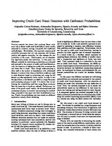
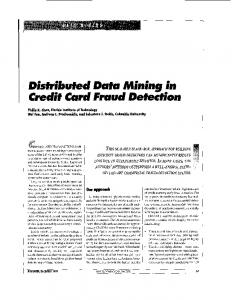
scores (between 0 and 1). The scores from each detector are combined using order statistics filters (the median and the minimum) and the mean. The resulting fused scores are used to calculate the classification performance of the system. Postprocessing steps such as extracting key performance indicators (KPI) for the company can be optionally performed. Some of these indicators are: VDR - Value Detection Rate (the total fraud percentage saved by the system for a certain cutoff values of score); ADR- Account Detection Rate (the percentage of detected cards); and ADT- Average Detected Transaction (the mean amount of transactions required for detecting a fraudulent card). IV. RESULTS AND DISCUSSION The data were provided by an internationally operating financial company. For confidentiality, this institution cannot be named. The real data consisted of 8,000,000 and 1,600 records of legitimate and fraud operations. The number of the variables was 8, corresponding to principal components extracted from the original variables of the records. Fig. 1 shows the results of the surrogate algorithm for legitimate operations. The first column on the left (Fig.1.a) shows 500 samples of the surrogate data, which has eight components. The second column (Fig.1.b) shows the histogram of the eight components in surrogate data, in black bars, with the histogram of the legitimate operations superimposed in red. The third column (Fig.1.c) compares the autocorrelations of each surrogate component (in blue) with the corresponding autocorrelation of the legitimate data (in red). Finally, the fourth column (Fig.1.d) shows the crosscorrelations of the first component with the other components (first seven rows) and the cross-correlation of the second component with the third component (eighth row). The crosscorrelations of the surrogate data are shown in blue, and the cross-correlations of the legitimate data are shown in red. It can be seen in Fig. 1 that the surrogate legitimate operations were very close to the real legitimate operations. The histograms in Fig. 1.b were very similar for surrogate and real operations, particularly for components 2 to 7. For components 1 and 8, even though the histograms are different, the results are still similar. The autocorrelations in Fig1.c were basically identical for real and surrogate data. Finally, the cross-correlations in Fig.1.d were harder to fit than the autocorrelations. However, for some cases the surrogate data obtained an almost exact fit of the cross-correlation function. Fig. 2 shows the results of the surrogate algorithm for fraud operations, and shows the same values than Fig.1. It can be seen that the surrogate fraud operations are close to the real fraud operations. The histograms of the surrogate data in Fig. 2.b were very close to that of the fraud data, particularly for the fourth component. They were less close to the real data than the histograms in Fig.1.b due the lower amount of fraud operations, which worsened the estimation of the parameters of the distributions. The autocorrelations of the surrogate fraud operations (Fig. 2.c) were very close to that of the real fraud operations. Finally, the cross-correlations in Fig. 2.d are similar for real and surrogate data.
3.b shows the same pdf, but calculated on surrogate legitimate data. Column Fig. 3.c shows the joint pdf of real legitimate operations for components 1 and 6 (first row), 1 and 7 (second), 1 and 8 (third), and 2 and 3 (fourth). Column Fig. 3.d shows the same pdf, but calculated on surrogate legitimate data.
Fig. 3 shows the joint probability density functions (pdf) of real and surrogate legitimate operations. Although the joint pdfs are calculated for the whole 8 components at once, they are shown in slices of two components to make the result more readable. Column Fig. 3.a shows the joint pdf of real legitimate operations for components 1 and 2 (first row), 1 and 3 (second), 1 and 4 (third), and 1 and 5 (fourth). Column Fig. 1
4000
0. 2
0
2000
0. 1
0 -0. 8
-1 0
50
1 00
1 50
200
250
300
350
400
450
500
-0. 6
-0. 4
-0. 2
0
0. 2
0. 4
0. 6
0. 8
0 -1 0
1
0. 1 0 -0. 1 -8
-6
-4
-2
0
2
4
6
8
-20
10
2
1 0000
0. 1
0. 05
0
5000
0. 05
0
-2
0 -1 0
0 0
50
1 00
1 50
200
250
300
350
400
450
500
0. 5
-6
-5
-4
-3
-2
-1
0
1
5000
0
50
1 00
1 50
200
250
300
350
400
450
0 -1 . 5
500
0. 5
-6
-4
-2
0
2
4
6
8
10
-1
-0. 5
0
0. 5
1
1.5
2
2. 5
3
5000
-1 0
-8
-6
-4
-2
0
2
4
6
8
10
0
50
1 00
1 50
200
250
300
350
400
450
0 -1 . 2
500
-0. 8
-0. 6
-0. 4
-0. 2
0
0. 2
0. 4
-1 0
0. 6
-0. 02 -20
-6
-4
-2
0
2
4
6
8
-20
10
4000
0. 04
0. 02
0
2000
0. 02
0
0
50
1 00
1 50
200
250
300
350
400
450
-1 1 0000
0
5000
-0. 5 0
50
1 00
1 50
200
250
300
350
400
450
-0. 5
0
-0. 2
0
0. 2
0. 4
0. 6
0. 8
0
50
1 00
1 50
200
250
300
350
400
450
0 -0. 8
500
-0. 6
-0. 4
-0. 2
0
0. 2
0. 4
0
50
1 00
1 50
200
250
300
350
400
450
-4
-2
0
2
4
6
8
10
-0. 6
-0. 4
-0. 2
a)
0
0. 2
0. 4
-1 0
0. 6
15
20
-1 5
-1 0
-5
0
5
10
15
20
-1 5
-1 0
-5
0
5
10
15
20
-1 5
-1 0
-5
0
5
10
15
20
-0. 02 -20
-1 5
-1 0
-5
0
5
10
15
20
-1 5
-1 0
-5
0
5
10
15
20
-1 5
-1 0
-5
0
5
10
15
20
-1 5
-1 0
-5
0
5
10
15
20
0. 05 0 -8
-6
-4
-2
0
2
4
6
8
10
-0. 05 -20 0. 02 0
-8
-6
-4
-2
0
2
4
6
8
10
-0. 02 -20 0. 1 0
0. 01 0
0 -0. 8
500
-6
0. 02
5000
-0. 5
-1 0
0. 6
1 0000
0
-8
0. 02 0. 01 0
0
0. 5
-1 0
1
5000
-0. 5
-1 0
0. 5
0. 03 0. 02 0. 01 0
0 -0. 4
500
0. 5
0
0
500
0. 5
10
-0. 1 -8
0. 5
-0. 5
5
0
0
-1
0
0. 1
0. 02
-0. 5
-5
0
0. 04
0
-0. 05 -20
-1 0
0. 02
0. 06 0. 04 0. 02 0
0 -0. 5
-8
-1 5
-8
-6
-4
-2
b)
0
2
4
6
8
10
-0. 1 -20
c)
d)
Fig. 1. Results of surrogate data from legitimate operations. 0. 2
400
0
200
-0. 2 0
50
1 00
1 50
200
250
300
350
400
450
500
0 -0. 5
2
1 000
0
500
-0. 4
-0. 3
-0. 2
-0. 1
0
0. 1
0. 2
0. 2 0. 1 0 -1 0
1
0. 1 0. 05 0 -1 0
0
-2 0
50
1 00
1 50
200
250
300
350
400
450
-6
500
-5
-4
-3
-2
-1
0
0. 05 0
-8
-6
-4
-2
0
2
4
6
8
10
-0. 05 -20
-8
-6
-4
-2
0
2
4
6
8
10
-0. 02 -20
400
0. 1
0. 05
0
200
0. 05
0
0
50
1 00
1 50
200
250
300
350
400
450
500
0 -1 . 4
1
200
0
1 00
-1 0
50
1 00
1 50
200
250
300
350
400
450
500
0 -0. 8
1
400
0
200
-1 0
50
1 00
1 50
200
250
300
350
400
450
500
0 -1 . 4
1
400
0
200
-1 0
50
1 00
1 50
200
250
300
350
400
450
500
0 -0. 6
-1 . 2
-1
-0. 8
-0. 6
-0. 4
-0. 6
-0. 4
-0. 2
-0. 2
0
0
0. 2
0. 2
0. 4
0. 4
0. 6
0 -1 0
0. 6
0. 06 0. 04 0. 02 0 -1 0
-8
-6
-4
-2
0
2
4
6
8
10
-1
-0. 8
-0. 6
-0. 4
-0. 2
0
0. 2
0. 4
-1 0
-8
-6
-4
-2
0
2
4
6
8
10
0. 2
0. 4
0. 6
0. 8
-1 0
-0. 05 -20
-0. 05 -20
-8
-6
-4
-2
0
2
4
6
8
10
-0. 02 -20
-8
-6
-4
-2
0
2
4
6
8
10
-20 0. 01
0
200
0. 02
0
50
1 00
1 50
200
250
300
350
400
450
500
0 -0. 6 200
0
1 00
-1 0
50
1 00
1 50
200
250
300
350
400
450
500
0 -0. 8
0 -0. 4
-0. 2
0
0. 2
0. 4
0. 6
0. 8
-1 0
-8
-6
-4
-2
0
2
4
6
8
10
-0. 6
-0. 4
-0. 2
0
0. 2
0. 4
0. 6
b)
-1 0
-1 0
-5
0
5
10
15
20
-1 5
-1 0
-5
0
5
10
15
20
-1 5
-1 0
-5
0
5
10
15
20
-1 5
-1 0
-5
0
5
10
15
20
-1 5
-1 0
-5
0
5
10
15
20
-1 5
-1 0
-5
0
5
10
15
20
-1 5
-1 0
-5
0
5
10
15
20
-0. 01 -20 0. 2
0. 03 0. 02 0. 01 0
a)
-1 5
-0. 01
0. 04
0
20
0
400
1
15
0. 01
1
-1
10
0
0 0
5
0. 02
0. 02 -0. 2
0
0
0. 04
-0. 4
-5
0. 05
0. 04 0. 02 0 -1 . 2
-1 0
0
0. 5
-0. 5
-1 5
0. 02
0
-8
-6
-4
-2
0
c)
2
4
6
8
10
-0. 2 -20
d)
Fig. 2. Results of surrogate data from fraud operations.
The results in Fig. 3 show that the surrogate legitimate data had a very similar joint pdf to that of real legitimate data. The peaks of the pdf for the surrogates were located at the same positions as the peaks of the pdf for the true data, and the shapes of both pdfs were very close in all cases. The pdf of the surrogates were more diffuse (i.e. less discrete), which might be caused by the amount of non-stationarity in the legitimate operations. Fig. 4 shows the pdf of real and surrogate fraud operations. As with Fig. 3, the pdfs are sliced to make the result more readable; the same slices were used in both Figures. The
surrogate algorithm obtained a similar pdf as that of the real operations, although the fit was a bit worse than that for legitimate operations. This was caused in part by the fact that the fraud data showed a more complex pdf than the legitimate operations. Furthermore, it is possible that the more diffuse pdf for the surrogates was also caused by the large amount of non-stationarity in fraud data. This is understandable, since fraudsters are constantly adapting to increase their chance to successfully defraud the banking companies.
-0. 6 -0. 4 -0. 2 0 0. 2 0. 4 -0. 5
0
0. 5
-0. 5
0
-0. 4
-0. 4
-0. 2 0
-0. 2 0
0. 2
0. 2
0. 5
-0. 5
0
0. 5
-0. 4
-0. 4
-0. 2
-0. 2
-0. 2
0
0
0
0
0. 2
0. 2
0. 2
0. 2
-0. 5
0
0. 5
-0. 5
-0. 2
-0. 2
0
0
0. 2
0. 2 -0. 5
0
0. 5
-0. 2 -0. 1 0 0. 1
0
0. 5
0
0
0. 5
0
0. 5
-0. 5
a)
0
-0. 5
0
0. 5
-0. 5
0
0. 5
-0. 5
0
0. 5
1
0
1
1
2
2
0. 5
0. 5
-0. 2 -0. 1 0 0. 1
0
-0. 2 -0. 1 0 0. 1 -0. 5
-0. 5
0. 5
0
-0. 2
-0. 2 -0. 1 0 0. 1 -0. 5
-0. 5
to obtain a low FPR. This is because false alarms correspond to negative experiences for the bank’s clients, which can affect its business. The results for this zone of interest with low values of FPR are shown in Fig. 6. The behavior of the ROC curves is similar in all cases, although there are some differences in value for very low amounts of FPR. In all cases, the lower the amount of surrogate operations, the closer the ROC became to that of the real operations. However, all the curves were very close for FPR above 0.06. Even if there were some differences for very low values of FPR, the curves with surrogates did not over-estimate the performance of the system, but instead obtained a reasonable (if low) estimate of the ROC with only real operations.
-0. 4-0. 2 0 0. 2 0. 4
b)
0.9
c)
d)
Fig. 3. Joint distribution of legitimate operations. -0. 2
-0. 2
-0. 2
0
0
0
0
0. 2
0. 2
0. 2
0. 2
-0. 2
-0. 05
0
0. 4
0. 05
-0. 4 -0. 2 0 0. 2
-0. 05
0
0. 05
-0. 4 -0. 2 0 0. 2 -0. 1 -0. 05 0 0. 05
-0. 4 -0. 2 0 0. 2 0. 4 -0. 1 -0. 05
0
0. 05 -0. 5
0
0
0. 5
0. 5 -0. 4
-0. 2
a)
0
0. 1
-0. 4
-0. 2
-0. 4 -0. 2
0
0
0. 2
0. 2 -0. 1
0. 05
0
-0. 1
-0. 4
0
0. 1
-0. 4 -0. 2 0 0. 2 0. 4 0. 6
-0. 1 -0. 05 0
-0. 5
0
-0. 2
-0. 1 -0. 05 0 0. 05 -0. 4 -0. 2 0 0. 2 0. 4
0. 4 -0. 1
0
0. 1
-0. 2
0
0
0
0. 2
0. 2 -0. 2
b)
0
c)
0. 2
0.5 0.4
Real data Surrogates 100% Surrogates 50% Surrogates 75%
0.3
0
0. 1
0
0
0.2
0.4 0.6 False Positive Rate
0.8
1
Fig. 5. ROC curves for different percentages of surrogate data. -0. 4
-0. 2
0.6
0.1 -0. 1
-0. 2
0.7
0.2
-0. 4 -0. 2 0 0. 2 0. 4 0. 6 -0. 4
0.8
-0. 4-0. 2 0 0. 2 0. 4
True Positive Rate
-0. 6 -0. 4 -0. 2 0 0. 2 0. 4
-0. 2
0
TABLE I.
-0. 2
0
0. 2
d)
Fig. 4. Joint distribution of fraud operations.
The similarity of the surrogates and the real operations was also tested by performing automatic fraud detection, using the method shown in [6]. The operations were split 50%/50% into training and testing. Detection performance was assessed using the ROC curves of the obtained fraud scores. To test the effect of the surrogate data on the classification, the detection was first performed only with real operations. Then, a certain amount of randomly-selected operations were replaced with surrogate operations and the detection was repeated. If the surrogates resemble the true data, the ROC curves will be similar. The amount of replaced operations was changed from 0% (only true operations) to 50%, 75%, and 100% (only surrogate operations). The obtained ROC curves are shown in Fig. 5. It can be seen that the curves are similar in all cases, particularly once the false positive rate (FPR) rises above 0.1. However, in the case of automatic fraud detection, it is of particular importance
AREA UNDER THE CURVE (AUC) OF THE DIFFERENT CONSIDERED CASES. AUC calculated on the:
Amount of surrogate data
Full ROC curves
Zoom in the detection zone of interest
0%
0.8708
0.0656
50%
0.8641
0.0640
75%
0.8563
0.0591
100%
0.8678
0.0589
This similarity between curves was also tested by calculating the area under the curve (AUC) for all the ROC curves. These values were calculated both for the full curves, and for the values within the zone of interest. The results are shown in Table I. It can be seen that the AUC is similar in all cases, although it is slightly higher for the case with no surrogate data. The difference is a bit more noticeable in the zone of interest, but it is very small once one considers the full ROC curves. These results are in concordance with Fig. 5 and Fig. 6, where the ROC curve with 0% surrogate operations rises higher than the other curves for very low values of FPR, but all the curves were very similar for FPR above 0.06.
0.7
ACKNOWLEDGMENT This work has been supported by Universitat Politècnica de València under grant SP20120646, Generalitat Valenciana under grant ISIC/2012/006; and Spanish Administration and European Union FEDER Programme under grant TEC201123403.
True Positive Rate
0.6 0.5 0.4
REFERENCES
0.3
[1]
Real data Surrogates 100% Surrogates 50% Surrogates 75%
0.2 0.1 0
0
0.02
0.04 0.06 False Positive Rate
0.08
0.1
Fig. 6. Zoom in the detection zone of interest of the ROC curves for different percentages of surrogate data.
V.
CONCLUSION
An application of surrogate techniques to enhance datasets for testing fraud detection algorithms has been presented. We have demonstrated that significant statistical characteristics (covariance, marginal distributions, and joint distributions as the original multivariate data) similar as the original multivariate data were obtained for the surrogate multivariate data. A fraud detection method for credit card operations was tested using the surrogate data. The detection results obtained for different mixtures of real and surrogate data were comparable under real requirements of very low false alarm. This work opens several possible financial applications of surrogates.
S. Bhattacharyya, S. Jha, K. Tharakunnel, and J. C. Westland, “Data mining for credit card fraud: A comparative study,” Decision Support Systems, vol. 50, pp. 602-613, 2011. [2] T. Schreiber and A. Schmitz, “Surrogate time series,” Physica D, vol. 142, no. 3-4, pp. 346–382, 2000. [3] D. Prichard and J. Theiler, “Generating surrogate data for time series with several simultaneously measured variables,” Physical Review Letters, vol. 73, no. 7, pp. 951–954, 1994. [4] P. Borgnat, P. Abry, P. Flandrin, "Using surrogates and optimal transport for synthesis of stationary multivariate series with prescribed covariance function and non-Gaussian joint distribution," Proceedings of IEEE International Conference on Acoustics, Speech and Signal Processing, ICASSP 2012, pp. 3729-3732, 2012. [5] C. Phua, V. Lee, K. Smith, and R. Gayler, "A comprehensive survey of data mining-based fraud detection research," Computer Research Repository, 2010. [6] A. Salazar, G. Safont, A. Soriano, L. Vergara, "Automatic credit card fraud detection based on non-linear signal processing," Proceedings of the 46th Annual IEEE International Carnahan Conference, Boston, USA, ICCST 2012, Article number 6393560, pp. 207-212, 2012. [7] H. Helgason, V. Pipiras, and P. Abry, “Fast and exact synthesis of stationary multivariate Gaussian time series using circulant embedding,” Signal Processing, vol. 95, no. 5, pp. 1123–1133, 2011. [8] J. Rabin, G. Peyr´e, J. Delon, and M. Bernot, “Wasserstein barycenter and its application to texture mixing,” in Proc. SSVM’11, 2011. [9] J.C. Bezdek, Pattern recognition with fuzzy objective function algorithms. Plenum Press, New York, 1981. [10] E.G. Learned-Miller, J.W. Fisher, “ICA using spacings estimates of entropy, Journal of Machine Learning Research,” vol. 4, pp. 1271-1295, 2003. [11] R. Duda, P. Hart, and D. Stork, Pattern Classification. John Wiley & Sons, New York, NY, USA, 2001. [12] A. Salazar, On Statistical Pattern Recognition in Independent Component Analysis Mixture Modelling. Springer Theses in Electrical Engineering Series, Springer-Verlag, Berlin, Heidelberg, 2013.