Symbol Knowledge Extraction from a Simple Graphical ... - CiteSeerX

2011 International Conference on Document Analysis and Recognition

Symbol Knowledge Extraction from a Simple Graphical Language Jinpeng LI, Harold MOUCHERE, Christian VIARD-GAUDIN IRCCyN (UMR CNRS 6597) - L’UNAM - Universit´e de Nantes, France {jinpeng.li,harold.mouchere,christian.viard-gaudin}@univ-nantes.fr segmentation process will have to be undergone, so that every basic graphical unit, termed as a grapheme, belongs to a unique symbol. Conversely, a symbol can be made of one or several strokes, which are not necessarily drawn consecutively, i.e. we do not exclude interspersed symbols. Then, these units are composed with some specific composition rules, to produce a symbol of the language, this symbol being an instance of a lexical unit. The problem is to identify from a large collection of handwritten scripts, all the lexical units based on the observation of the strokes. Some of them corresponding directly to a symbol, others are only a part of a symbol. Eventually, the same kind of stroke according to the context will be either a single symbol or a piece of a more complex symbol. Let us illustrate the concept with a simplified example. Assume that we observe only two kinds of strokes: horizontal stroke and vertical stroke {‘−’, ‘|’}. In a first model, consider also, that the only composition rule is the left to Right rule (R). Then, it is possible to produce this kind of string : “| − | | | − | | | − | | | ”. Based on all the available strings in the training dataset, we would like to be able to define a lexicon, i.e. a list of lexical units, which will allow to describe in an optimal way the entire corpus. With this example, two possible lexicons would be L = {“| − |”, “|”} or L = {“| − | |”, “|”}. A similar problem is studied in unsupervised language acquisition [1]; the lexicon is extracted from texts, considered as a sequence of characters. But suppose now, that we add two new composition rules: the Below rule (B) and the Intersection rule (I). Then, with these two-dimensional spatial relations in addition to sequences of strokes, we are able to compose more complex messages, such as “| + | = ||”. In this case, the search space for the combination of strokes which forms possible symbols is much more complex since it is no longer a linear one. We give an overview of the proposed system in section II, then the extraction of the graphemes and of their spatial relationships are presented in section III. We describe the algorithm which is used to build the lexicon in section IV, before presenting the experimental results in section V.

Abstract—In this paper, we study the problem of symbol knowledge extraction. We assume that some unknown symbols are used to compose a handwritten message, and from a dataset of handwritten samples, we would like to recover the symbol set used in the corresponding language. We applied our approach on online handwriting, and select the domain of numerical expressions, mixing digits and operators, to test the ability to retrieve the corresponding symbol classes. The proposed method is based on three steps: a quantization of the stroke space, a description of the layout of strokes with a relational graph, and the extraction of an optimal lexicon using a minimum description length algorithm. At the symbol level, a recall rate of 74% is obtained on the test dataset produced by 100 writers. Keywords-online handwriting; knowledge extraction; minimum description length; spatial relation;

I. I NTRODUCTION The knowledge of symbols which compose a given language is something essential to recognize, and then to interpret a handwritten message based on this language. For this reason, most of the existing recognition systems, if not all, need the definition of the character or symbol set, and require a training dataset which defines the ground-truth at the symbol level so that a machine learning algorithm can be trained on this task to recognize symbols from handwritten information. Many recognition systems take advantage from the creation of large, realistic corpora of ground-truthed input. Such datasets are valuable for the training, evaluation, and testing stages of the recognition systems. They also allow for comparison between state-of-the-art recognizers. However, collecting all the ink samples and labelling them at the stroke level is a very long and tedious task. Hence, it would be very interesting to be able to assist this process, so that most of the tedious work can be done automatically, and that only a high level supervision need to be defined to conclude the labelling process. In this respect, we propose to extract automatically the relevant patterns which will define the lexical units of the language. This process is carried out from the redundancy in appearance of basic regular shapes and regular layout of these shapes in a large collection of handwritten scripts. For the targeted application, which will be defined in more details further and which is related to online numerical expressions, we consider that the strokes, a sequence of points between a pen-down and a pen-up, are the basic units. Should this assumption not be verified, then an additional 1520-5363/11 $26.00 © 2011 IEEE DOI 10.1109/ICDAR.2011.128

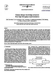
II. OVERVIEW This section introduces the overview of the extraction of lexicon. Given a handwriting database, Fig. 1 pictures our scheme to extract the lexicon of symbols. This scheme 608

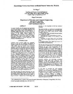
The second step extracts the spatial relations between the strokes. We predefine three generic spatial relations, right (R), below (B) and intersection (I). We choose the top-left stroke as the first stroke to start. To build the relational graph, we have considered from each node (stroke) the outcome of at most 2 possible edges when relation B and/or R are satisfied and only one edge when relation I (with a higher priority) is encountered. In other words, I is exclusive with R and B. The edges are oriented towards the nearest strokes for the considered relation. In this way, we obtain a directed acyclic graph (DAG). All the nodes in the graph can be travelled by several possible paths (sequences). Thus given a handwriting database containing expressions {ei }, it is transformed into a set of sequences of graphemes/relations {sqj }. This transformation bridges the gap between the graph and sequences. For example Fig.2 illustrates a DAG from an expression. The graphemes are marked by the indices of strokes in equation to avoid the ambiguity since several strokes share the same grapheme. In this example, all the nodes in the graph can be travelled by two possible paths (sequences), (2(0) , R, ..., −(4) , R,  (6) , I, |(7) ) and (2(0) , R, ..., −(4) , B, −(5) , R,  (6) , I, |(7) ). In the next section, we explain how to extract the lexicon from these sequences.

Database

Clustering Graphemes

23 8|

1.Quantization

8 3 8 8 2 | | 2.Extraction of spatial relations Lexicon B

Relational Graphs

:Grapheme B :Below

Figure 1.

=

3.Extraction of lexicon

Lexicon extraction overview

contains three principal steps, quantization of strokes, extraction of spatial relations between strokes, and extraction of lexicon. First, we code each stroke using a finite set of graphemes. This is a quantization step. The second step, extraction of spatial relations, analyses spatial relations between the strokes. For instance, “=” is composed of the two same graphemes “−” with the spatial relation below “B” which corresponds to the following subsequence (−, B, −). These graphemes and spatial relations are organized in a relational graph inspired by a symbol relation tree (SRT) [2]. From the relational graph, the sequences containing graphemes and spatial relations are extracted, they are next processed by the third step, which computes the lexicon. The main idea of the developed algorithm is to use the frequency of subsequence of graphemes/relations to detect symbols. If the subsequence (−, B, −) is very frequent, we could consider (−, B, −) as a lexical unit. In fact, a lexical unit usually represents a ground-truth symbol. We mainly focus in this work on the problem from the relational graph to the lexicon and its evaluation. Thus the generation of the relational graph is briefly described.

IV. E XTRACTION AND U TILIZATION OF THE L EXICON We use the iterative algorithm proposed in [5] to build the lexicon from the sequence of graphemes/relations. The principal idea of this algorithm is to minimise the description length of sequences by iteratively trying to add and delete a word, in terms of Rissanen’s minimum description length (MDL) principle [6]. The MDL principle means that the best lexicon minimise the description length of the lexicon and that of the observation; in our case the observation is the sequence of graphemes/relations. A. Extraction of the Optimal Lexicon We describe a simple example inspired by [1] to give a general idea of the minimum description length principle. The aim is to find the lexicon [5] using MDL principle. We analyse the expression “1234 − 2/1234” as the sequence of graphemes U = (1, 2, 3, 4, −, 2, /, 1, 2, 3, 4). For simplicity, the spatial relations are omitted but they are taken into

III. E XTRACTION OF G RAPHEMES AND S PATIAL R ELATIONS For the quantization of strokes, we firstly extract the graphemes. Since the stroke is a sequence of points, we apply the dynamic time warping (DTW)[3] distance as the similarity of shape between two strokes. Clustering techniques are used for the generation of the codebook. Many different algorithms are available for this task. Instead of using a traditional k-means algorithm, we prefer an agglomerative hierarchical clustering since the tree topology is favourable to tune easily the number of prototypes. Furthermore the Lance-Williams formula [4] provides an efficient computational algorithm for hierarchical clustering. Once the graphemes (prototypes) are selected with the hierarchical clustering, all the strokes are tagged with the virtual label of the closest grapheme using the DTW distance.

R

2(0)

R

8(3)

I

(1)

"+"

| (2)

R

"4" (4)

R

(6)

I

|

(7)

:Grapheme :Spatial Relation R :Right B :Below I :Intersection :Segmentation

2+8=4 (4) (5)

(1)

"="

(0)

B

Figure 2.

609

(5)

(2)

(3)

R

Example of relational graph of “2 + 8 = 4”

(6)

(7)

account in the real algorithm. In Table I, we have three lexicons, L1 , L2 and L3 to interpret U by Viterbi representation [1]. Intuitively L2 is the best lexicon since L2 contains the word “1234”.

U:

Considering the lexicon L2 = {(1), (2), (3), (4), (−), (/), (1, 2, 3, 4)}, L2 has a hierarchical structure; (1), (2), (3), and (4) compose the longer sequence (1, 2, 3, 4) defined by (1) ◦ (2) ◦ (3) ◦ (4) = (1, 2, 3, 4) where ◦ is the concatenation. The Viterbi representation is used to interpret U by matching the longest sequence in L2 shown in Fig. 3. For example, U is interpreted by L2 as (1, 2, 3, 4)◦(−)◦(2)◦ (/)◦(1, 2, 3, 4). C(.) is defined as the number of occurrences on the level of coding of U and coding of L2 . For instance, C((2)) = 2 since “01” in “111 110 01 101 111” composing U and “01” in “000 01 001 100” composing (1, 2, 3, 4), shown in Table I. To find the number of occurrences, it can be obtained by the out-degree of each member from Viterbi representation in Fig. 3. The numbers of occurrences of the other members are that C((1, 2, 3, 4)) = 2, C((1)) = C((3)) = C((4)) = C((−)) = C((/)) = 1 from Viterbi representation. According to the numbers of occurrences, we encode U and L2 by Huffman coding which is minimum redundancy [7]. Therefore we can get the description length of U and L2 . The description length of L2 is 25 bits which is the minimum description length among the three lexicons.

Figure 3.

B. Segmentation Using Optimal Lexicon Here we explain how to obtain a segmentation of a new expression using the computed optimal lexicon L. A new expression e is transformed into one or more sequences of graphemes/relations from the relational graph, e → {sqk }. We get the segmentation from the {sqk } by the Viterbi representation with the optimal lexicon L. In fact, the segmentation from {sqk } contains the spatial relations, I, R, and B. These spatial relations are used to define the lexicon since (−, B, −) is different of (−, I, −), but are not necessary for the segmentation of strokes. The segmentation of the complete expression is the result of merging segmentation from each path. For example in Fig. 2, because of the two paths from the relational graph, we get two sets of segmentation in graph using the optimal lexicon, {(2(0) , R), (−(1) , I, |(2) ), (R, 8(3) , R, −(4) , R), ( (6) , I, |(7) )} and {(2(0) , R), (−(1) , I, |(2) ), (R, 8(3) , R), (−(4) , B, −(5) ), (R), ( (6) , I, |(7) )}. We simplify the segmentation in graph by deleting the spatial relations. The two sets of segmentation will be simplified as: and {{2(0) }, {−(1) , |(2) }, {8(3) , −(4) }, { (6) , |(7) }} {{2(0) }, {−(1) , |(2) }, {8(3) }, {−(4) , −(5) }, { (6) , |(7) }}. The sequences are converted into sets since the link between graphemes of spatial relations is missed. The union of these two sets is the segmentation of the equation, { {2(0) }, {−(1) , |(2) }, {8(3) , −(4) }, {8(3) }, {−(4) , −(5) }, { (6) , |(7) } }. We define this union of segmentations as s(e, L) with the optimal lexicon L. However there may be two members in s(e, L) which are intersected but not included which means conflict. For example, the two sets of {8(3) , −(4) } and {−(4) , −(5) } conflict with −(4) noted by: CB({8(3) , −(4) }, {−(4) , −(5) }). We call the conflict as CB since the brackets are crossing. We solve this conflict by tracing back to C((8(3) , R, −(4) )) and C((−(4) , B, −(5) )) in lexicon and by keeping the bigger C(.) in sequences of graphemes/relations; the other set is deleted. Probably we keep {−(4) , −(5) } since C((−(4) , B, −(5) )) > C((8(3) , R, −(4) )). Therefore we get the segmentation for the equation in Fig. 2, { {2(0) }, {−(1) , |(2) }, {8(3) }, {−(4) , −(5) }, { (6) , |(7) } }. We also make the segmentation as a hierarchical structure from the hierarchical lexicon L. Finally we get the segmentation defined by S(e, L) = {{2(0) }, {−(1) }, {|(2) }, {8(3) }, {−(4) }, {−(5) }, { (6) }, {|(7) }, {−(1) , |(2) }, {−(4) , −(5) }, { (6) , |(7) }}. This hierarchical structure provides us with

An algorithm to build the optimal lexicon is presented in [5] using MDL principle. We try to iteratively add or delete a word in order to minimise the description length until the lexicon cannot be changed. Thus we get an optimal lexicon L on the training handwriting database containing the sequences of graphemes/relations {sqj }. Table I T HREE LEXICONS FOR THE SEQUENCE OF GRAPHEMES U = (1, 2, 3, 4, −, 2, /, 1, 2, 3, 4) L1 Viterbi representation of U : Huffman coding of U : Code length of U and L1 : L2 Viterbi representation of U : Huffman coding of U : Inner representation of (1, 2, 3, 4): Huffman coding of (1, 2, 3, 4): Code length of U and L2 : L3 Viterbi representation of U : Huffman coding of U : Inner representation (1, 2, 3, 4, −, 2, /, 1, 2, 3, 4): Huffman coding of (1, 2, 3, 4, −, 2, /, 1, 2, 3, 4): Code length of U and L3 :

Viterbi representation

{(1), (2), (3), (4), (−), (/)} (1) ◦ (2) ◦ (3) ◦ (4) ◦ (−)◦ (2) ◦ (/) ◦ (1) ◦ (2) ◦ (3) ◦ (4) 00 10 01 110 1111 10 1110 00 10 01 110 28 bits {(1), (2), (3), (4), (−), (/), (1, 2, 3, 4)} (1, 2, 3, 4) ◦ (−) ◦ (2)◦ (/) ◦ (1, 2, 3, 4) 111 110 01 101 111 (1) ◦ (2) ◦ (3) ◦ (4) 000 01 001 100 25 bits {(1), (2), (3), (4), (−), (/), (1, 2, 3, 4, −, 2, /, 1, 2, 3, 4)} (1, 2, 3, 4, −, 2, /, 1, 2, 3, 4) 1111 (1) ◦ (2) ◦ (3) ◦ (4) ◦ (−)◦ (2) ◦ (/) ◦ (1) ◦ (2) ◦ (3) ◦ (4) 100 00 101 01 1110 00 110 100 00 101 01 33 bits

610

grammar information, i.e. {{ (6) , |(7) }} → {{ (6) }, {|(7) }}. In a word, given a handwriting database {ei }, we transformed {ei } to sequences of graphemes/relations {sqj } and then extracted an optimal lexicon L from these sequences. Considering a new expression e, we obtained the segmentation S(e, L) in terms of the lexicon L. At the end we cleaned the conflict in segmentation and made the segmentation as the hierarchical structure S(e, L).

2+8=4

(6)

(7)

Example of measures

In order to validate our approach, we have produced a dataset of handwritten numerical expressions from a large set of isolated handwritten symbols, and we evaluate the performance by the four measures presented in the previous section. A. Description of the Database

|S(e, G) ∩ S(e, L)| = , |S(e, G)|

To test the performance of our approach, we created an artificial database named Calculate[8]. Firstly the expressions in Calculate are generated in terms of the grammar N1 op N2 = N3 where N1 , N2 and N3 are numbers composed of 1, 2 or 3 digits from {0, 1, ..., 9}. The distribution of number of digits for Ni={1,2,3} is 70% of 1 digit, 20% of 2 digits and 10% of 3 digits randomly. In addition, op represents the operators {+, −, ×, ÷}. Fig. 5 shows an example in Calculate that N1 , N2 , N3 and op contain 3 digits, 1 digit, 2 digits and “×” respectively. Secondly Calculate is separated into a training part and a test part. The training part contains 897 expressions from 180 writers for the unsupervised learning. On this part we extracted the graphemes by clustering and extracted the lexicon by the iterative search algorithm [5]. The test part contains 497 expressions written by another 100 writers. Learned graphemes and lexicon are tested on this part.

where |.| is the cardinality of a set. The recall rate evaluates the percentage of right segmentation which are found in ground-truths. On the contrary the second measure RCB calculates the percentage of crossing brackets in S(e, G) compared with the S(e, L). And RCB is defined by: |{A|A ∈ S(e, G), ∃B ∈ S(e, L), CB(A, B)}| . |S(e, G)|

RCB reveals the error of the segmentation of L compared with ground-truths. The third measure is defined by RLost = 1 − RRecall − RCB . RLost means the percentage of segments (symbols) in S(e, G) which are not found. Note that these 3 measures are because of the hierarchical structure of the resulting segmentation. Thus we define a fourth measure based on the segmentation found by the Viterbi representation using the longest words: RGood =

(3)

V. E XPERIMENTS

Our objective is to verify if our extracted segmentation correspond to a human made segmentation S(e, G) (groundtruths). We evaluate the performance of segmentation with lexicon L by four measures from [1]. The first is recall rate:

RCB =

(2)

Figure 4.

C. Measures

RRecall

(4) (5)

(1)

(0)

|{A|A ∈ S(e, G), ∃B ∈ T op(S(e, L)), B = A}| |S(e, G)|

B. Results and Discussion On the training part of Calculate, we firstly extract all the prototypes of strokes (graphemes). To illustrate the next step, we first select 150 prototypes. Then we evaluate different numbers of prototypes. At the end, we evaluate the performance of the optimal configuration on the test part of Calculate. Using 150 prototypes, we try iteratively to add and delete a word with the lexicon in terms of the algorithm in [5]. The lexicon starts with 153 words (150 prototypes plus 3 spatial relations). At the end it stops at 498 iterations with 504 words since none of decrease of description length can be made. Fig. 6 describes the accuracy of segmentation from four measures, RRecall , RGood , RCB and RLost during the unsupervised learning of the lexicon on the training part of the database. The best accuracy RGood of 65% is reported in the 20th iteration and then it decreases slowly. According

where T op(S) = {D|D ∈ S, ∀E ∈ S, E = D, D ⊂ E} which extracts a set of the longest possible segments without inclusion. Thus RGood evaluates the performance of Viterbi representation. To explain the proposed measures, we use a new lexicon Lm giving the hierarchical structure segmentation S(e, Lm ) = {{2(0) }, {−(1) }, {|(2) }, {8(3) }, {−(4) }, {−(5) }, { (6) }, {|(7) }, {−(1) , |(2) }, {2(0) , −(1) , |(2) }, {8(3) , −(4) }} as illustrated in Fig. 4. The ground-truths are defined by S(e, G) = {{2(0) }, {−(1) , |(2) }, {8(3) }, {−(4) , −(5) }, { (6) , |(7) }}. The recall rate is that RRecall = 3/5 = 0.6; the ground-truths {2(0) }, {−(1) , |(2) } and {8(3) } are found. The crossing bracket rate RCB is 0.2 as the ground-truth {−(4) , −(5) } is crossing with the segmentation {8(3) , −(4) }. RLost is 0.2 since the ground-truth { (6) , |(7) } is lost. The RGood is zero because none of ground-truth is found by Viterbi representation. Although RGood is zero, the RRecall = 0.6 reveals some grammar information in expression, for instance, {2+} → {{2}, {+}} and {+} → {{|}, {−}}.

N1

Figure 5.

611

op N2 =

N3

A numerical expression from the Calculate database

1

0.8

0.9

0.7 0.65 0.6

RecallRate

CBRate

LostRate

GoodRate

0.8 0.7

RecallRate GoodRate CBRate LostRate

0.4

0.6

Rate

Rate

0.5

0.5 0.4

0.3

0.3

0.2 0.2

0.1 0 0 20

0.1 0

100

Figure 6.

200 300 Number of iterations

400

500

15

30

75

120

150

225

300

450

Number of prototypes

Figure 7.

Accuracy of segmentation

to RCB and the overlap of RGood and RRecall , our system does not make any error before the 20th iteration but it leaves 35% of symbols lost in terms of RLost . After 20th iteration, RRecall keeps increasing until the end of iteration, but RGood decreases gradually. It means that the new added word does not represent symbols but frequent sequences of symbols or of parts of symbol. At the end of iteration RRecall , RCB , RLost and RGood are 77%, 10%, 13% and 61% respectively. To find the optimal number of prototypes of strokes, Fig. 7 shows the rates for different numbers of prototypes at the end of the lexicon extraction; no more word can be added and deleted. The best RRecall of 78% is reported using 120 prototypes (RCB = 10%, RLost = 12%, RGood = 62%). RCB always decreases since more and more different prototypes of strokes are found. RGood remains fluctuating roughly around 60% after 75 prototypes. The compromise best number of prototypes is 120 because of the high RRecall and RGood and the low RCB and RLost . Next we test the learned lexicon using 120 prototypes of strokes on the test part of Calculate. RRecall of 74%, RCB of 10%, RLost of 16%, RGood of 63% are reported. RGood is comparable to that on the learning part. These results show the robustness of our lexicon. In the field of unsupervised learning on texts, the similar problem of segmentation is studied a lot. Thus we compare the recall rate in handwritten expressions with that in texts. Using the same learning method of description length in [5], RRecall of 90.5% and RCB of 1.7% are reported respectively on an English corpus, Brown corpus [9]. Although our RCB of 10% is much higher than that in texts, but we get a fair RRecall of 74%. VI. C ONCLUSION

Rates for different numbers of prototypes on the training part

is generated artificially from handwritten isolated symbols written by different writers. The grammar of Calculate is very simple and only one-line expressions exist. Therefore if we increase the complexity of handwriting database, we may need some new spatial relations. Then the relational graph becomes more complicated and we will need some graph mining techniques as for example in [10]. Hence, more complicated graph languages like flowcharts could be addressed in our future work. Acknowledgment: This work is supported by the French R´egion Pays de la Loire in the context of the DEPART project www.projet-depart.org. R EFERENCES [1] C. D. Marcken, “Unsupervised language acquisition,” Ph.D. dissertation, Massachusetts Institute of Technology, 1996. [2] T. H. Rhee and J. H. Kim, “Efficient search strategy in structural analysis for handwritten mathematical expression recognition,” Pattern Recognition, vol. 42, no. 12, pp. 3192 – 3201, 2009. [3] V. Vuori, “Adaptive methods for on-line recognition of isolated handwritten characters,” Ph.D. dissertation, Helsinki University of Technology (Espoo, Finland), 2002. [4] G. N. Lance and W. T. Williams, “A General Theory of Classificatory Sorting Strategies: 1. Hierarchical Systems,” The Computer Journal, vol. 9, no. 4, pp. 373–380, 1967. [5] C. D. Marcken, “Linguistic structure as composition and perturbation,” in In Meeting of the Association for Computational Linguistics. Morgan Kaufmann Pub., 1996, pp. 335–341. [6] J. Rissanen, “Modeling by shortest data description,” Automatica, vol. 14, no. 5, pp. 465 – 471, 1978. [7] D. Huffman, “A Method for the Construction of MinimumRedundancy Codes,” Proceedings of the IRE, vol. 40, no. 9, pp. 1098–1101, Sep. 1952. [8] A. M. Awal, “Reconnaissance de structures bidimensionnelles : application aux expressions math´ematiques manuscrites enligne,” Ph.D. dissertation, Ecole polytechnique de l’universit´e de Nantes, France, 2010. [9] N. W. Francis and H. Kuˇcera, Frequency Analysis of English Usage: Lexicon and Grammar. Boston: Houghton Mifflin, April 1982, vol. 18, no. 1. [10] D. J. Cook and L. B. Holder, “Substructure discovery using minimum description length and background knowledge,” J. Artif. Int. Res., vol. 1, pp. 231–255, February 1994.

In this paper we presented an unsupervised learning method of lexicon on simple handwritten mathematical expressions. Firstly the graphemes are extracted by agglomerative hierarchical clustering. Secondly the graphs of spatial relation are generated inspired by SRT, and these graphs are transformed into sequences. We extracted the lexicon from these sequences by reducing the description length. At the end, we got a recall rate of 74% on the test part of our database. Furthermore, the database Calculate 612