Symbolic field theory with Cadabra Kasper Peeters
[email protected] Cadabra is a new computer algebra system designed specifically for the solution of problems encountered in field theory. It has extensive functionality for tensor polynomial simplification including multi-term symmetries, fermions and anticommuting variables, Clifford algebras and Fierz transformations, implicit coordinate dependence, multiple index types and many more. The input format is a subset of TEX. Both a command-line and a graphical interface are available.
Introduction
muting ones. Space-time dependence of the fields is often implicitly assumed. Indices come in many types (vector, spinor, Lie-algebra valued) and are often suppressed in order to make the expressions readable. Thus, converting field theory expressions from their TEX-based de-facto standard notation to a general purpose computer algebra language is often cumbersome, and translating the answer back again introduces further sources of error.
In theoretical physics, many problems are described by making use of the concept of a “field”. A field associates scalar, vector or generic tensor degrees of freedom to every point in space or in space-time. A familiar example is the electromagnetic field, which is described by a vector at every space-time point. Another example is the gravitational field, which is a two-index symmetric tensor field. Physics problems then involve equations of motion for these fields, or invariant charges constructed from them, or symmetry transformations, or various other manipulations. Often problems involve Grassmann-valued fields, or tensors transforming under other groups than the Lorentz or rotation group, and so on. Manipulating such tensorial expressions could certainly benefit from computer algebra. However, there is a number of characteristic features of “field theory problems” which often make them unsuited for a direct solution using standard general purpose symbolic computer algebra systems. There are several reasons for this. One of them is that tensorial expressions are typically “graphs”: the indices of the tensors can be contracted (dummy indices) and thus form closed loops in the expression. This is in contrast to the “list” data type often used in general purpose computer algebra systems. This basic but important fact often quickly leads to problems when one tries to build tensor manipulation packages on top of general purpose systems. A second problem is the fact that tensors often have symmetries (e.g. symmetry or anti-symmetry in indices, but commonly more complicated ones, like the Bianchi or Ricci identities familiar from differential geometry). This makes that converting an expression to a canonical form, especially when there are also anti-commuting tensors present, often goes beyond what general purpose systems can handle. A third problem is the fact that field-theory notation is extremely compact, and translations to general purpose algebra systems often cumbersome. Non-commuting products, for instance, occur frequently (e.g. for fermionic fields) without any specific notational difference to com-
Characteristic features Cadabra is a new system which was designed from scratch as a general purpose system for field theory problems. In order to achieve this, several things are done differently from many other general purpose systems. Perhaps the most immediately visible aspect of Cadabra is that it accepts field theory expressions written directly in (a subset of) TEX. This makes notebooks particularly easy to read; see e.g. the screenshot of the graphical interface displayed below.
Greek symbols, tensor indices, derivative operators and so on are all entered in a natural form. 1
In order to attach meaning to symbols, Cadabra uses the concept of “properties”. A symbol can e.g. be declared to have a certain symmetry property in its indices, or have the property that it is anti-commuting with other symbols in a list. More complicated properties, such as “Spinor”, which combine various properties in one easy to remember shortcut, exist as well. Properties go beyond simple data types in the sense that more than one property can be attached to a symbol, and there are also properties which are attached to lists of symbols (e.g. a property “Indices” which makes symbols part of a set of indices). Tensor polynomial expressions, including those containing anti-commuting and non-commuting tensors or tensors carrying indices which transform under different symmetry groups, are canonicalised using some of the most powerful algorithms currently available. These algorithms deal not only with simple symmetry or antisymmetry, but also with multi-term symmetries such as Bianchi or Ricci identities. Moreover, the user can specify the sort order of symbols so that expressions can be automatically canonicalised according to the way in which they look most natural. Dummy indices never need to be relabelled by hand, as all algorithms, including the various substitution commands, automatically take care of index relabelling. The program knows about many concepts which are common in field theory. It handles anti-commuting and non-commuting objects without special notations for their products, it knows about gamma matrix algebra, Fierz identities, Dirac conjugation, vielbeine, flat and curved, covariant and contravariant indices, implicit dependence of tensors on coordinates, partial and covariant derivatives. It has extensive facilities for handling of field theory expressions, e.g. dealing with variational derivatives. It features a substitution command which correctly handles anti-commuting objects and dummy indices and offers a wide variety of pattern matching situations which occur in field theory. Finally, the program is (apart from a few dependencies on other freely available libraries and programs), entirely standalone. It is written in C++ and the manual contains documentation on how to extend the system with new algorithms.
This shows how to declare index groups and input a simple expression. We now perform a substitution @substitute!(%)( B_{a b} ->
C_{a b c} D_{c} );
The result is Aab Cbcd Dd ; Index relabelling has automatically taken place. Also note how the substitute command has figured out that B_{a b} on the left-hand side is equivalent to B_{b c}, without any explicit wildcards or patterns. Indices are automatically understood to be patterns, i.e. their explicit names do not matter. Indices can be simple letters, as in the example above, but it is also perfectly possible to put accents on them. The following example illustrates this. A_{\dot{a} \dot{b}}::AntiSymmetric. A_{\dot{b} \dot{a}};
Ab˙ a˙ ; @canonicalise!(%);
(−1) Aa˙ b˙ ; Here we also see a second usage of property declarations: the construction in the first line declares that the Aa˙ b˙ tensor is antisymmetric in its indices. The canonicalise command subsequently writes the input in a canonical form, which in this trivial example simply means that the indices gets sorted in alphabetical order. Continuing the example above, one can also use subscripts or superscripts on indices, as in the example below. {a_{1}, a_{2}, a_{3}, a_{4}}::Indices(vector). V_{a_{1}} W_{a_{1}}: @substitute!(%)( V_{a_{2}} -> M_{a_{2} a_{1}} N_{a_{1}} );
Ma1 a2 Na2 Wa1 ; As is clear from these examples, commands always start with a ‘@’ symbol. The ‘!(%)’ bit attached to the commands roughly means that the command should be applied at all levels (the ‘!’ mark) on the previous expression (the ‘%’ sign). Input lines normally end with ‘;’, but output can be suppressed by using ‘:’ instead (as in the last example). Let us now look at two more complicated examples. The first one we will discuss is the computation of the product of Dirac gamma matrices. Consider the product
Examples Having given a formal introduction to the system, the best way to exhibit the usefulness is by simply discussing a few examples. Let us first look at a few simple substitution commands to get familiar with the basics. The output in the examples is exactly how things appear in the graphical user interface.
Γsr Γrl Γkm Γms , where Γrs is the anti-symmetrised product of two Dirac gamma matrices, i.e. objects satisfying the algebra {Γr , Γs } = 2δrs . We want to write this product in terms of Kronecker delta symbols and fully antisymmetrised gamma matrices. This problem starts by declaring the index objects and other symbols,
{ a, b, c, d }::Indices. A_{a b} B_{b c};
Aab Bbc ; 2
two polynomials of the Weyl tensor,
{s,r,l,k,m,n}::Indices(vector). {s,r,l,k,m,n}::Integer(0..d-1). \Gamma_{#}::GammaMatrix(metric=\delta). \delta_{m n}::KroneckerDelta.
1 Eij = −Ci mkl Cjpkq Cl pmq + Ci mkl Cjmpq Ckl pq 4 1 − Cikjl C kmpq C l mpq , 2 1 E = Cjmnk C mpqn Cp jk q + Cjkmn C pqmn C jk pq . 2 satisfy, when evaluated on an Einstein space, the identity
The declaration in the first line involves a ‘list property’, which attaches the property to the entire list rather than the individual symbols. The declaration for the gamma matrix shows that we are defining an object with implicit indices: the spinor indices will be suppressed. The notation _{#} denotes the presence of an arbitrary number of indices. Next follows the input,
1 ∇i ∇j Eij − ∇i ∇i E = 0 . 6 This is a tedious exercise with Bianchi identities when done by hand, but is handled with Cadabra with relative ease. First we declare indices and other objects,
\Gamma_{s r}\Gamma_{r l} \Gamma_{k m}\Gamma_{m s}:
Expanding the product of two basis elements is done by applying the following command (which is postfixed with ‘!!’ indicating that the algorithm should be applied until the result no longer changes)
{i,j,m,n,k,p,q,l,r,r#}::Indices(vector). C_{m n p q}::WeylTensor. \nabla{#}::Derivative. \nabla_{r}{ C_{m n p q} }::SatisfiesBianchi. Eij:=- C_{i m k l} C_{j p k q} C_{l p m q} + 1/4 C_{i m k l} C_{j m p q} C_{k l p q} - 1/2 C_{i k j l} C_{k m p q} C_{l m p q}:
@join!!(%){expand}:
(−1)((2Γlr − Γlr d + δlr d − δlr ) (2Γkr − Γkr d + δkr − δkr d));
E:= C_{j m n k} C_{m p q n} C_{p j k q} + 1/2 C_{j k m n} C_{p q m n} C_{j k p q}: exp:= \nabla_{i}{\nabla_{j}{ @(Eij) }} - 1/6 \nabla_{i}{\nabla_{i}{ @(E) }}:
We need only a few more steps to obtain the final result: distributing the product over the sums, joining gamma matrices once more, and then factorising the result:
Note in particular the way in which derivatives are declared and entered into the system. We now need to apply the Leibniz rule twice to expand the derivatives, and then sort the tensors and write the result in canonical form with respect to mono-term symmetries,
@distribute!(%); @join!(%){expand}; @distribute!(%); @factorise!(%){d}; @collect_factors!(%);
@distribute!(%): @prodrule!(%): @distribute!(%): @prodrule!(%):
Γkl (12 − 18d + 8d2 − d3 ) + δkl (−3 + 6d − 4d2 + d3 );
@prodsort!(%): @canonicalise!(%): @rename_dummies!(%): @collect_terms!(%):
One of Cadabra’s features which is clearly visible above is that the program does not try to do anything smart unless it is explicitly told to do so. This is manifest from the fact that e.g. the ‘collect factors’ command had to be entered explicitly, but the logic goes even further. The above example in fact makes use of a default set of simplification algorithms, which can be specified with
Because the identity which we intend to prove is only supposed to hold on Einstein spaces, for which the divergence of the Weyl tensor vanishes, we substitute @substitute!(%)( \nabla_{i}{C_{k i l m}} -> 0 , \nabla_{i}{C_{k m l i}} -> 0 );
Note once more how the substitution command automatically deals with index relabelling: neither the dummy index i nor the open indices have to match in order for the substitution to apply; the only relevant information is the contraction pattern. We now get a long list of terms,
::PostDefaultRules( @@prodsort!(%), @@eliminate_kr!(%), @@canonicalise!(%), @@collect_terms!(%) ).
Such default rules can be added and removed at will, allowing for a fine-grained control over computations. Cadabra was originally written as a tool to solve problems in gravity and supergravity, so it has extensive support for symbolic calculations with curvature tensors and related objects. The last example which we will discuss shows some of this. We want to verify that the following
Cijmn Cikmp ∇q ∇j Cnkpq − Cijmn ∇k Cipmq ∇p Cjqnk + ... . This expression should vanish upon use of the Bianchi identity. By expanding all tensors using their Young projectors, this becomes manifest: 3
@young_project_product!(%): @sumflatten!(%): @collect_terms!(%);
A more extensive introduction to the implementation details can be found in [3].
The result is zero, proving what we set out to show. Readers interested in seeing more examples are referred to [1] or the sample notebooks available on the web site [2]. A mailing list for discussions about Cadabra is also available.
Current users The origin of Cadabra lies, as mentioned before, in research in supergravity and related areas. After the first public announcement to the high-energy physics community in January 2007 [1], various other physicists have started using the program, often for ‘simple’ day-to-day calculations but especially also for more extensive research projects. The program has found applications in areas such as beyond-the-standard-model physics, gravity and supergravity, string theory and quantum field theory in general. Because the program has, apart from its graphical user interface, also a command line version, it is possible to run large batch jobs. In this form, the system has been used on a large Linux cluster at the Albert-EinsteinInstitute in Potsdam for several gravity-related problems. From the various forms of feedback received during the last half a year, it has become clear that the ease of use, in combination with the convenient graphical notebook interface, are what set Cadabra apart from other systems. Given the considerable attention which Cadabra has attracted (the web site receives around a thousand hits per month), there is a demonstrated need for the continuing development of this “field theory friendly” computer algebra system.
Under the hood Cadabra was written, and rewritten several times, over the course of the last five years. The basis is formed by an expression tree manipulation core, which however is tightly coupled to algorithms which offer “graph-like” views of the tree. More precisely, this means that there are several internal mechanisms by which the tree can be inspected; it is for instance possible to iterate over all indices of an object, but it is also possible to iterate only over those which are uncontracted or to iterate over all indices including those which are carried by operators wrapping the symbol, as in e.g. ∂a Bcd . On top of this core lies a set of algorithm modules, each of which can be called from the user interface or directly from within C++. The property system is implemented using a C++ inheritance tree, and the way in which properties can be combined together in the user interface is thus a direct consequence of the standard C++ inheritance mechanism. This includes, in particular, multiple inheritance. Except for a very small number of predefined symbols (\prod and \sum for instance), all other ones obtain their characteristics from properties. The graphical notebook user interface is built using the gtkmm library, and directly calls LATEX to typeset output expressions. It has a multiple-view system and allows users to cut and paste output expressions, either back into the notebook as input or directly as LATEX source into e.g. a paper. The interface runs both on Linux and Mac OS X systems. For batch jobs or other tasks for which the graphical interface is less useful, the kernel can also be used directly as a command line application.
Literature [1] K. Peeters, “Introducing Cadabra: a symbolic computer algebra system for field theory problems”, arXiv:hep-th/0701238. [2] Cadabra web site, www.aei.mpg.de/∼peekas/cadabra [3] K. Peeters, “A field-theory motivated approach to computer algebra”, Comp. Phys. Comm. 176 (2007) 550-558, arXiv:cs.CS/0608005.
4