Synchronisation Primitives for Highly Parallel Discrete ... - CiteSeerX

Proceedings of the 32nd Hawaii International Conference on System Sciences - 1999 Proceedings of the 32nd Hawaii International Conference on System Sciences - 1999

Synchronisation Primitives for Highly Parallel Discrete Event Simulations Jon Kerridge1, Peter Welch2, and David Wood2 Department of Computing, Napier University Edinburgh UK 2 Computing Laboratory, University of Kent, Canterbury UK [email protected], {P.H.Welch, D.C.Wood}@ukc.ac.uk 1

Abstract A new set of synchronisation primitives is described that simplify the control of very large numbers of fine-grained parallel processes, such as those arising from discrete event modelling systems. The new primitives are derived from the multi-way event synchronisation and choice defined in Hoare’s algebra of Communicating Sequential Processes (CSP). One of them, EVENT, provides for dynamically structured and multiple barrier synchronisation that is completely deterministic in its semantics. Another, christened BUCKET, provides for an explicitly non-deterministic version of an EVENT, where the non-determinism is triggered by a programmable internal action (such as a timeout). The paper shows how these primitives may be combined with standard CSP channel communication to design and implement a highly parallel model of an urban traffic network (as an example). The model is simple to create and understand, being object-oriented with components that directly reflect objects on the ground (such as roundabouts and traffic lights). The performance and scalability both of the primitives and of the traffic model are discussed in terms of their implementation on an inexpensive DEC Alpha based multiprocessor (plug-in boards and a standard PC). Overheads for managing channel communications and the EVENT/BUCKET primitives are shown to be very light (less than one microsecond), so that the direct execution of highly-parallel designs remains efficient down to very fine levels of granularity. An example is presented that operates more than 100 times faster than real-time on a single processor, context-switching at more than a quarter of a million times per second. Going multi-processor allows larger models to be executed at similar speeds. Feedback from such models enables different kinds of analysis to tried ahead of real-time -for example, predictive ‘what-if’ experiments after some major road traffic accident -- so that the most effective remedial strategies can be found and adopted within real-time.

1 Motivation The simulation of systems involving large numbers of discrete events has been a topic of research for a long time. The normal approach is to identify each event in the model and the parameters that govern its behaviour. A time step based solution is then applied which determines the progress that each event would make in each time step and identifies the interactions that take place between events. The simulation proceeds by repeated evaluation of each event for a sequence of time steps. Such techniques have been applied to meteorological prediction, fluid flow models. oil reservoir modelling and the modelling of similar phenomena. The main problem with this approach is that the size of the time-step and the number of discrete events in the model determine the accuracy of the model. As the time step is reduced and the number of modelled events increases the computational requirement grows in order (n2) time. Parallel solutions have therefore been adopted where the model is distributed over the processors making up

the parallel platform so that each processor deals with a disjoint subset of the events. The fundamental model, namely stepping through a sequence of time steps over a number of events has however not changed. In many cases parallelisation has permitted larger and more accurate model construction running in the same time as previous single processor models. In some real world systems not every event in the model is going to contribute to the overall result at every time step and thus some of the calculations undertaken are not absolutely necessary. An example of such a system is a model of a road traffic network where stationary vehicles do not contribute to modelling movement, though they are an important determinant of congestion within the complete road network. Paramics[1] is an important example of a road network model that has been developed from a sequential model and has been parallelised by distributing the compute load over a number of processors, typically on a CRAY T3D. The underlying basic model has however not been changed. Paramics has been used mainly for strategic

0-7695-0001-3/99 $10.00 (c) 1999 IEEE

1


planning of arterial road networks and for example the complete trunk road network of Scotland has been modelled. In the research reported in this paper we were looking for a solution that could be implemented on a modestly priced workstation and which could thus be used for tactical decision making by road traffic engineers in realtime. We wished to develop a tool which could be used to evaluate a number of different control strategies faster than real-time so that the ‘best’ strategy could be implemented to deal with a specific problem. Examples of such problems include the aftermath of major incidents such as road traffic accidents and the chaos caused by other emergency situations. We also wanted a tool that was sufficiently flexible that it could be used to develop control strategies for forthcoming events such as road works which have a serious effect on traffic flow in an urban network. Finally, the tool could be used to evaluate proposed changes to the road traffic network. For this functionality to be generally available to road traffic engineers on a regular basis the solution had to be available at workstation prices so that each road traffic management authority could sensibly consider its purchase. Recent environmental legislation in the UK requires traffic authorities to close roads in periods of poor air quality. The specific effect of the road closures have to be evaluated and appropriate control strategies have to be invoked if the pollution is just not moved to another part of a network. A tool such as that outlined in this paper would provide an appropriate method of developing such strategies and then monitoring how they work in practice during such road closures. The tool also has then benefit of enabling strategy revisions in real-time if the current strategy is found not to be working.

1.1 Previous Work In order to build such a system we developed a highly parallel microscopic model of an urban traffic network[2]. This model was based upon Hoare's Communicating Sequential Process[3,4,5] (CSP). The road space is split up into slots of 5.75meters, which is the average amount of space occupied by a passenger car in the UK at rest in a queue[6]. Each slot is implemented using a process which waits for a vehicle to enter, determines for how long the vehicle will occupy the slot given current road conditions, waits for that amount of time and then attempts to move to the next slot. In order to make modelling simpler, collections of slots make up traffic lanes and other features such as intersections, pedestrian crossing points, bus stops and other road network constituents. These collections are also implemented as processes and thus a large number of processes can result for a typical urban network. In our first version of this model, processes that were in the waiting state were placed on a queue of such processes that was maintained

in time order. Thus as soon as the time for a process to restart occurred, it was added to the set of running processes and could continue execution. The main problem with this architecture is that processes which are added to the time queue have to be placed in the correct time sequence which means manipulating a linked list which is very costly when the number of processes on the queue is large. We therefore sought a different way of maintaining this timing information. A traffic network can be modelled in terms of time intervals which in computing terms are relatively long. We need to know how long a vehicle remains in a slot to an accuracy of at most one hundredth of a second and possibly a tenth of a second will suffice. The timer queue was accurate to the microsecond or less, depending upon the implementation. A further difficulty of using an inbuilt timer mechanism is that there is a classic problem of synchronising real timers across multiple processors. It was crucial that this aspect was considered from the outset as we wanted a model that was guaranteed to scale. We thus developed the EVENT and BUCKET primitives described in the next section. Our approach to parallel discrete event simulation (PDES) is similar to that of [7] except that the computational model we employ requires no micro-kernel or lightweight thread mechanism to provide resource sharing amongst the processes. Like [7] we directly support the logical processes of the simulation by processes in the computational model. The underlying communication primitives and process model in our model is directly supported by the abstract machine which executes on a bare machine with no operating system. Unlike many PDES systems, such as [8] we do not require buffers in our logical procsses because the underlying computational model (CSP) does not require buffered communication. A process becomes idle until it can complete a communication with a neighbouring process. Thus we implement each virtual process of the simulation as a process in its own right and then use the communication model to ensure correct interaction between the logical processes. This leads to a simple, but highly parallel, description of the system being modelled. Rather than adopting a time warp [9] or similar PDES approach, we have used a discrete multi-element clock system that can be distributed over any number of processors. Each logical process of the simulation determines for how long it will occupy the resource it is simulating given the current state of the resource. The logical process then suspends itself by placing its process reference in the appropriate element of the clock relative to the current element of the clock. In sequence, each of these elements is accessed and any (logical) processes in the element are re-started. Each re-started process executes either until it suspends itself in another element of the clock or attempts a communication with another

0-7695-0001-3/99 $10.00 (c) 1999 IEEE

2


process that is not yet ready to receive that commincation. The clock requires as many elements as are required to effect the longest delay in the simulation. The granularity of the clock depends upon the system being simulated which in our traffic system is one tenth of a second. While a (logical) process of the simulation is waiting to communicate or is suspended in an element of the clock it consumes no processor resource. We shall also show that the cost of resuming a set of (logical) processes, from a clock element, is very low and independent of the number of processes being resumed. Our approach is also similar to that of [10] in that we use barrier synchronisations similar to that of Bulk Synchronous Parallel programming. The main difference is that our synchronisation events vary in size depending upon the number of processes that are resumed with each element of the clock. In addition to the logical processes of the simulation, we require only a small number of additional processes. One to collect data from the simulation, one to synchronise global simulated time and one process per processor to organise and manipulate the multi-element clock on that processor. Each processor has exactly the same sized multi-element clock.

2 The Synchronisation Primitives A BUCKET [11] is a place where all processes that are to commence processing at the same time are put until that time arrives. The processes in a BUCKET are flushed from the BUCKET as and when the time arrives to recommence these processes. The effect of flushing a BUCKET is to place all the processes on the processor run queue so that they can be executed. A time sequence is obtained by having a vector of such BUCKETs and the BUCKETs are flushed in order with cyclic wrap around. A process that wishes to be delayed for a certain period of time calculates the displacement from the current bucket that has just been flushed and falls into the bucket, later in the sequence, that will give the required delay. The mechanism of falling into a bucket has to be very low cost as it is going to occur many times during a simulation and must not depend on the number of processes already in the bucket. Similarly, the mechanism of flushing a bucket must also be of similarly low cost and ideally the cost should be independent of the number of processes waiting in the bucket. The modelling can now be disassociated from any concept of real processor time. Once all the processes that have been flushed from a BUCKET have done as much work as they are able, the next BUCKET can be flushed without having to wait. Determining when the flushed processes have completed as much work as possible is the role of the EVENT [12] primitive. EVENT is a lightweight synchronisation barrier and we can have many EVENTs in the same system. Processes can synchronise on the

EVENT and only when all expected processes have synchronised can the individual processes continue to process beyond the synchronisation point. For our traffic model two EVENTs are used - one to control local operations within a processor and the other to synchronise all the processors. When a BUCKET is flushed, a local EVENT is initialised with the number of processes in the BUCKET. Each of these processes then executes until it can go no further at which point it synchronises on the EVENT. When all the flushed processes have synchronised on the EVENT the next BUCKET can be flushed. The bucket mechanism can be equated to real-time quite easily by assuming that each bucket in the sequence corresponds to the next unit of time. Thus if we need a maximum delay of 30 seconds and an accuracy of one tenth of a second, a sequence of 300 BUCKETs is required. Each time the sequence is traversed corresponds to 30 seconds of real time. Within the model time can be determined to the tenth by noting which bucket in the sequence is currently being processed. Global synchronisation over a number of (non-shared memory) processors can be achieved quite simply. Each processor is registered with the global EVENT barrier. At the end of each cycle of the sequence of BUCKETs, the process managing the BUCKET data structure synchronises on this global EVENT, which enables synchronisation across the processors. Once every processor has synchronised, each of the individual processors can continue for another cycle. Thus, the maximum amount that any processor can be out of synchronisation with its neighbours is governed by the number of buckets in an individual processor’s BUCKET sequence. Normally, this would be the same size on each processor. For some environments no discrepancy can be sustained and thus a global EVENT synchronisation would be required after the flushing of each BUCKET.

2.1 Occam Binding for EVENT and BUCKET CSP is a mathematical theory for specifying and verifying complex patterns of behaviour arising from interactions between concurrent objects. Developed by Tony Hoare in the light of earlier work on monitors, CSP has a compositional semantics that greatly simplifies the design and engineering of such systems -- so much so, that parallel design often becomes easier to manage than its serial counterpart. CSP primitives have also proven to be extremely lightweight, with overheads in the order of a few hundred nanoseconds for channel synchronisation (including context-switch) on current microprocessors [13,14]. The results reported in this paper were obtained using this occam binding. Recently, the CSP model has been introduced into the Java programming language [15,16,17,18,19]. Implemented as a library of packages [20,21], JavaPP

0-7695-0001-3/99 $10.00 (c) 1999 IEEE

3


[19] enables multithreaded systems to be designed, implemented and reasoned about entirely in terms of CSP synchronisation primitives (channels, events, etc.) and constructors (parallel, choice, etc.). This allows 20 years of theory, design patterns (with formally proven good properties - such as the absence of race hazards, deadlock, livelock and thread starvation), tools supporting those design patterns, education and experience to be deployed in support of Java-based multithreaded applications[22]. The current versions of Java are not yet fast enough for us to use for the fine-granularity of modelling described in this paper, but the JavaPP binding for CSP makes it a future candidate.

2.1.1 EVENT DATA TYPE EVENT RECORD INT Fptr, Bptr: INT active, count: :

The EVENT primitive is based upon a data structure which comprises two pointers which maintain a linked list of processes that have already synchronised on an EVENT instance[12]. Fptr points to the front of the list and Bptr points to the end of the list which is the place where synchronising processes are added to the list. The data structure also contains two other variables; active which holds the number of processes which synchronise on an event instance and count which indicates how many processes have synchronised on an EVENT instance. The value Null is a special value to indicate that a pointer contains no valid address because no process pointer can ever take that value. VAL INT Null IS MOSTNEG INT:

The procedure initialise.event sets the pointers and other variables of an EVENT to a predefined state and in particular sets the values of active and count. It has been declared as INLINE so that it is expanded in the code like a macro rather than being called like a procedure to make invocation more efficient. INLINE PROC initialise.event (EVENT e, VAL INT count) e := [Null, Null, count, count] :

When a process wishes to synchronise on an EVENT it calls the synchronise.event procedure. In all but the last case this results in the blocking of the calling process, adding its process reference pointer to the linked list of other such processes maintained by the EVENT data structure and decrementing the count field. If the synchronising process is the last one expected, signified by e[count] = 0, then all the processes which have been enqueued on the linked list can now execute and so

are appended to the processor’s run queue (a unit time operation). The last synchronising process continues execution. The EVENT is then re-initialised by setting the list pointers to Null and resetting e[count] to the value in e[active]. In section 2.2 we show that this can be achieved very efficiently provided the workspace associated with a process is well structured. INLINE PROC synchronise.event (EVENT e) SEQ e[count] := e[count] - 1 IF e[count] = 0 SEQ ... append the whole e-queue to the run-queue ( see section 2.2) e := [Null,Null,e[active],e[active]] TRUE SEQ ... enqueue this process on e-queue ... save instruction pointer and schedule next process :

2.1.2 BUCKET The BUCKET primitive is a non-deterministic version of the EVENT primitive[11]. The main difference is that an EVENT always expects the same number of synchronising processes, whereas the BUCKET does not know this as it depends upon the dynamics of the model being executed. Thus the BUCKET record does not have an active field and the count field starts at zero and increments. DATA TYPE BUCKET RECORD INT Fptr, Bptr: INT count: : INLINE PROC initialise.bucket (BUCKET b) b := [Null, Null, 0] : INT INLINE FUNCTION number.in.bucket (VAL BUCKET b) VALOF SKIP RESULT b[count] :

When a process wishes to deschedule itself into a BUCKET it does so by calling particular fall.into.bucket. INLINE PROC fall.into.bucket (BUCKET b) SEQ b[count] := b[count] + 1 ... enqueue this process on b-queue ... save instruction pointer and schedule next process :

0-7695-0001-3/99 $10.00 (c) 1999 IEEE

4


When the processes in a bucket can be released to run, by adding them to the processor’s run queue, a process calls the flush.bucket procedure. INLINE PROC flush.bucket (BUCKET b) SEQ ... append the whole b-queue to the run-queue ( see section 2.2) b := [Null, Null, 0] :

2.2 Implementation The work reported in this paper has been undertaken using the Kent Retargettable occam Compiler (KRoC) [23] which enable the use of occam on processors other than transputers. These details are significant only to explain the very low overheads for BUCKET and EVENT implementations in KroC, around 500ns for each operation on a modern micro-processor ( eg a 235MHz DEC Alpha). In the transputer implementation of occam[24] a very efficient process workspace layout was adopted that minimised the amount of process state that needed to be saved when a process context switch occurs. A process switch can occur when a process communicates, waits on a timer or is de-scheduled as a result of processing for longer than a maximum time slice. KRoC maintains the same basic process workspace structure shown in figure 1, regardless of target architecture. Work Space (WS)

set of processes on a linked list would have the structure shown in figure 2, where Fptr and Bptr have the use described earlier. This structure is used for all linked lists in the KRoC implementation of occam including the processor run queue. It is also used for EVENT and BUCKET variables. Hence, adding a (non-empty) set of processes that have synchronised on an EVENT or a BUCKET to the run queue requires the following sequence, where RUN represents the run queue and M is the memory space of the processor. M[RUN[Bptr]] := EVENT[Fptr] RUN[Bptr] := EVENT[Bptr]

This is of course independent of the number of processes on either queue. The only other state that has to be saved is the process’s instruction pointer which is stored in the location immediately below the Wptr location. A process is executed by taking the first process from the run queue as follows, ignoring the case when the run queue is empty. Ireg := M[RUN[Fptr]-1] Wreg := RUN[Fptr] RUN[Fptr] := M[RUN[Fptr]]

Ireg and Wreg are two registers in the processor. No other state has to be recovered to allow processing to commence as no other processor registers contain useful state when a process is descheduled.

2.3 Combining Primitives

Wptr Process Control Block (PCB) Figure 1 The workspace is split into two parts relative to the workspace pointer (Wptr). Above Wptr is the space used by the process during execution organised as a stack. Below Wptr is a fixed size space used to hold pointers and other values when a process is descheduled, the precise content of which is not germane to the description, for details see [25]. WS

WS

WS

PCB

PCB

PCB

Fprt

Bptr Figure 2 The location pointed to by Wptr is however crucial as it is used to implement a linked list of processes. Thus a

In processes that are using communication, EVENT and BUCKET synchronisation, care must be taken to ensure that they are preserved in the correct state. In particular, when a process attempts to communicate then two situations apply. First, if the process is the first to attempt a particular communication between a pair of processes then it must wait until the other process is ready to communicate. This must also result in a synchronisation EVENT being sent to signify that the process has undertaken as much processing as it possibly could. Secondly, if the process is the second one to communicate in a communication pair then the communication takes place and data is transferred between the processes. The other process is added to the run queue and the process continues execution and thus does not yet synchronise on the EVENT. Additional procedures have been created which determine the state of a communication. These either cause EVENT synchronisation, if this is the first process to communicate, or undertake the communication, if it is the second, and continue execution without synchronising. It may happen that a process could continue execution until it needed to fall into another bucket. In this case the

0-7695-0001-3/99 $10.00 (c) 1999 IEEE

5


process must EVENT synchronise before it falls into the next bucket. INLINE PROC input.or.synchronise ( CHAN OF ANY c, []BYTE data, EVENT e, BOOL synchronised ) IF synchronised c ? data TRUE INT state: SEQ ... determine state of channel c IF state = Null -- not ready SEQ synchronise.event ( e ) synchronised := TRUE TRUE SKIP c ? data -- communicate in any case :

The effect of the procedure input.or.synchronise is to check its last parameter to determine whether the process calling the procedure has already synchronised. If this is the case then the communication can continue without any other interaction. If the calling process has not yet synchronised then it is necessary to determine the state of the communication channel. If the channel is not ready to communicate, then the calling process must synchronise on its EVENT because the process has now undertaken as much work as it could - it can then undertake the communication. If the channel is ready to communicate the communication is completed and the calling process continues execution without synchronising on the EVENT. There is an equivalent procedure for undertaking output on a channel in a process that accesses an EVENT.

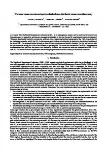
3 Modelling a Road Traffic Roundabout A roundabout is modelled as a collection of slots, each having a specific task as shown in Figure 3. The arrival process (A*) receives vehicles from an adjacent lane, waits until the required conditions are met for the vehicle to enter the roundabout and then communicates with the I process to which it is connected to send the vehicle details onto the roundabout, thereby commencing the passage of the vehicle around the roundabout. The required conditions for a vehicle to enter the roundabout (assuming that vehicles drive on the left hand side of the road) are, using the slots marked with a *: I is empty and one of the following alternatives is holds : E* and I* are both empty E* empty and I* contains a vehicle that is exiting the roundabout at D* E* contains a vehicle exiting at D* and I* is empty E* and I* both contain vehicles exiting through D*

An ingress process (I) accepts a vehicle from either of its connected A or E processes and then passes the vehicle on to the next E process. An egress process (E) determines whether the vehicle is departing from the roundabout at the arm of the roundabout which it is approaching. If this is the case, the E process sends the vehicle to the D process otherwise it is sent to the connected I process. A depart process (D) accepts inputs from its connected E process and then sends the vehicle to the first slot of its adjacent lane. In the model, as implemented, it is assumed that vehicles travel round a roundabout at constant speed and that they can accelerate to this speed within the space of the arrival slot. Each of the roundabout processes is based upon a basic slot process which is used to construct a lane, described in the next section.

A

I

D

E

D

A

E

I

I

Slot in adjacent lane

E*

A* D*

Roundabout slot

Figure 3

E

D

I*

A Internal Roundabout Processes A - Arrive D - Depart I - Ingress E - Egress

3.1 The Basic SLOT Process A basic slot process is used to construct a traffic lane. Each slot represents about 5.75m of road space. A lane comprises the required number of slot processes which relate to the length of the lane. A lane also requires two further processes, not discussed here, one which gathers data which gives the state of the lane and the other is used to control the movement of vehicles between the slots that make up the lane. In the code for the slot process, the parameter b is a vector of type bucket and contains the number of buckets needed by the model. The parameter current.bucket indicates which element of b is being processed currently. The event parameter local.sync is used to synchronise all the processes that have been flushed from the bucket that is currently being processed. The parameter occupancy holds details of all the slots in the feature to which this slot process belongs. Thus in a lane the occupancy vector

0-7695-0001-3/99 $10.00 (c) 1999 IEEE

6


holds vehicle details ( type VD) for all the slots of the lane. In a roundabout the occupancy vector holds information about each occupied slot in the roundabout feature. The access to these variables has been organised so that only one process ever writes to the shared variable though several are able to read them. The channels in and out are used respectively to receive an incoming vehicle’s details from a previous slot and to send them to the next slot. The data type VD holds details about a vehicle such as its type, the driving behaviour of its driver in different situations, the route the vehicle would normally take and the time at which the journey started. The variable synchronised is used to remember, on a particular cycle through the while loop, that the process has synchronised on local.sync because each slot process must only synchronise once on each cycle. PROC slot ( VAL INT slot.id, INT current.bucket, []BUCKET b, EVENT local.sync, CHAN OF VD in, out, []VD occupancy ) BOOL synchronised: SEQ synchronised := FALSE fall.into.bucket(b[0]) VD data IS occupancy[slot.id]: WHILE TRUE INT to.wait, t.in.tenths: SEQ input.or.synchronise ( in, data, local.sync, synchronised ) 1 ... determine time to wait in this slot to.wait := ( current.bucket + t.in.tenths ) \ (SIZE b ) 2 IF NOT synchronised synchronise.event ( local.sync ) 3 TRUE SKIP fall.into.bucket ( b[to.wait] ) 4 synchronised := FALSE output.or.synchronise ( out, data, local.sync, synchronised ) 5 data := VD.empty 6 :

Initially, the process inputs an incoming vehicle if it is available. If there is no incoming vehicle it synchronises on local.sync and then waits for the incoming vehicle (1). Once a vehicle has been input the value of data is updated. The amount of time that the vehicle would occupy the slot is determined. In the current version of the model this time is calculated to an accuracy of 0.1 seconds and each bucket corresponds to 0.1 seconds. The variable to.wait holds the bucket number into which this process should fall (2). If the process has not yet synchronised on local.sync then this is now forced (3), after which the process falls into the required bucket (4) and synchronised is reset to false. In due course the bucket into which this process has fallen will be flushed

by a local.time.organiser process ( see section 3.3 ) at which point the vehicle details will be output to the next slot. If the next slot is still occupied then this communication cannot immediately complete and so the process must be able to synchronise at this point as well (5). Finally the data value is updated to indicate that the slot is now empty (7). It should be noted that the model contains no explicit means of modelling queues of traffic, as a queue naturally emerges from the model because a vehicle will remain in a slot as long as the next slot is occupied. This is a major difference between this traffic model and other currently available models because they spend much of their processing time determining the precise dynamics of queues. In addition this model determines the time a vehicle will stay in a slot by applying the laws of motion based upon the amount of empty space in front of a vehicle and the speed of the vehicle immediately in front. Previous work [26] has shown that it is also possible to build into the model the specific dynamics associated with joining the back of a queue of vehicles which are controlled by traffic lights.

3.2 Roundabout Specific Processes The roundabout is simply instantiated as a set of processes running in parallel corresponding to those shown in Figure 3. In addition, a further process is required to output the occupancy vector to a results collection process. In the model described here this data is collected every 0.3 seconds, of simulated time, from every lane and feature that make up the network model. Again, this output.occupancy process uses the bucket mechanism to determine its delay. The amount of data collected can be varied and be from something as simple as the slot occupancy information to complete details of the vehicle in every slot. In addition the output.occupancy process can create further statistics pertaining to the occupancy of the feature which can also be collected. PAR output.occupancy PAR i = 0 FOR 4 PAR rbout.ingress rbout.arrival rbout.egress rbout.depart

( ... )

( ( ( (

...) ... ) ... ) ... )

3.3 Managing Time Two simulated-time management processes are required; one which synchronises time across all the processors that are used to implement the model and the other synchronises processes on a single processor.

0-7695-0001-3/99 $10.00 (c) 1999 IEEE

7


PROC global.time.synchronise ( EVENT global.time.sync, INT cycles, VAL INT p, CHAN OF BOOL init ) BOOL go: SEQ init ? go WHILE TRUE SEQ synchronise.event(global.time.sync) cycles := cycles + 1 :

The process global.time.synchronise is instantiated on one processor only and counts the number of times there has been such a global synchronisation in the parameter cycles. This value can then be used to recover the actual time when activities occur within the model. Assuming each bucket corresponds to a 0.1 second delay then the time of an activity in seconds from the start of running the model is given by : ( (cycles * ( SIZE b))

+ current.bucket ) / 10

where b is the bucket variable. The process local.time.organiser initially synchronises on the global.time.sync event (1) so that all the processors start at the same time. Thereafter the process runs in a never ending loop. The initial action is to ensure that all the data that is being output as a result of output.occupancy processes being scheduled from the previous bucket have completed (2). The local.time.organiser process is only executed when all the processes that were scheduled from the previous bucket flushing have synchronised on local.time.sync. The next action is thus to determine the number of processes in the current bucket (3). The event local.time.sync must be initialised with the number of processes (nib) which have to synchronise (4). The additional process is the local.time.organiser process itself. The bucket identified by current.bucket is then flushed (5) which adds all the processes in that bucket to the processor run queue. The local.time.organiser then synchronises on the local.time.sync event (6) which causes the process to be descheduled until all the flushed processes have themselves synchronised. At this point we have to force the local.time.organiser to the back of the run queue to ensure that all the processes that were flushed from the bucket can progress as far as is possible. This overcomes a possible race-hazard that can occur between a process synchronising on an EVENT and then falling into the bucket which would be the next bucket to be flushed. In the slot process (lines 4 and 5) it is possible for a process to synchronise on an event and then be

descheduled before it can fall into a bucket - leading to a possible race hazard. The voluntary pre-emption of local.time.organiser is achieved by calling RESCHEDULE (7). PROC local.time.organiser ( INT current.bucket, []BUCKET b, EVENT local.time.sync, global.time.sync, SEMAPHORE result.s ) SEQ synchronise.event ( global.time.sync ) 1 WHILE TRUE INT nib: SEQ ... ensure all result processing complete for this cycle 2 nib:=number.in.bucket ( b[current.bucket] ) 3 initialise.event ( local.time.sync, nib + 1 ) 4 flush.bucket (b[current.bucket]) 5 synchronise.event ( local.time.sync ) 6 RESCHEDULE() 7 current.bucket:=(current.bucket + 1) \ max.syncs 8 IF current.bucket 0 SKIP TRUE synchronise.event(global.time.sync)9 :

Once this state has occurred the value of current.bucket is incremented (8). This value wraps round so that it is always in the range of the number of buckets in the vector b. If the value of current.bucket has reached zero then a synchronisation takes place on global.time.sync (9) to ensure that all processors remain in step.

3.4 The Complete Network Model The instantiation of the complete model is given in outline below. All the global shared variables which comprise the bucket vector and all the events are initialised; after which the model can be started in parallel. In this example, one instance of a single lane roundabout is started together with four vehicle stream generators, one for each input lane to the roundabout. Eight lanes are then started each containing 20 slots. This system runs on a single processor and thus only one instance of the local.time.organiser and global.time.synchronise processes are required. A process which collects the results from each of the lanes and the single.lane.roundabout is instantiated together with a process which puts data onto the screen and provides a rudimentary user interface for testing the system.

0-7695-0001-3/99 $10.00 (c) 1999 IEEE

8


SEQ ... initialise anything that’s shared PAR single.lane.roundabout ( ... ) PAR i = 0 FOR 4 generate.vehicle.stream ( ... ) PAR i = 0 FOR 8 lane.20 ( ... ) local.time.organiser ( current.bucket, b, local.time.sync, global.time.sync, results.s ) global.time.synchronise ( global.time.sync, global.cycles, 2, init ) results.collector ( data.out, stdout, stdout.s ) test.interface ( ... ) :

4 Performance Evaluation The performance of the model described above has been measured on an Alpha Data [27] DEC alpha based processor board plugged into a PC. The alpha processor is rated at 235Mhz. Vehicles were input into the system from a vehicle stream generator based upon a random number generator. In all cases the same seed was used for the generator so that each measurement would use exactly the same input vehicle streams. Figure 3 shows two networks, one with two roundabouts and the other with five, used to measure performance. These were compared with a single isolated roundabout. Two different timings were taken, in all cases the model was allowed to run until 20 vehicles were output from one of the lanes. The number of vehicles output on the other lanes would be less than 20.

A program was written which analysed the output file to determine how many movements there were of vehicles from one slot to the next and how many times data was collected. From this analysis we can determine the number of deschedules per second that were taking place during the running of the simulation. Each slot transition incurs 4 process deschedules comprising 2 communications, one event synchronise and one fall into a bucket. Each data collection incurs a semaphore deschedule, one communication and one fall into a bucket deschedule. The program which analysed the data output file was not able to detect a transition if there has been a vehicle movement that involved two vehicles moving together such that the second vehicle occupies the slot vacated by the first. Due to the nature of the data this will tend to reduce the number of vehicle movements detected, particularly for the more complex networks. This fact therefore accounts for some of the reduction in deschedules per second as the networks get more complicated. The column Speed-up gives the performance improvement of Execution Time 2 compared with Simulated Time. Table 1 M Simulat- Execution Time Speed File Descheded Time 1 2 Up i/o ules 1 145.6 1.14 0.09 1617 78 241422 2 147.8 1.93 0.19 777 88 228515 5 163.5 3.89 0.34 480 87 195488 M: 1 single roundabout 2 two roundabout network 5 five roundabout network

5 Conclusions

Figure 3 Two different execution timings in seconds (see Table 1) were taken for each network as follows: 1. Visualisation data, comprising occupancy data for every slot in the network, was collected every 0.3 seconds of simulated time and saved 2. The same data was collected but not saved to file The Simulated Time column shows in seconds the actual time it would have taken for the vehicles to move round the network, until the termination condition was reached. The file input-output rate (KB/sec) is calculated in terms of the difference between the two times divided into the size of the file created.

The single, most important conclusion to be drawn is that it is possible to build a traffic model that can be executed in a PC environment, admittedly using an add-in processor, that will be able to model reasonably complex networks much faster than real time. It is reasonable to expect that a network of 2400 features would run in approximately real-time. Thus by the addition of extra processors faster than real-time performance would be expected. This means that the technology could be used in an urban traffic network control centre to evaluate a number of strategies after an incident to determine the ‘best’ strategy which could then be implemented well before congestion starts to occur. Traffic control systems commonly collect data on a five minute cycle. Thus several simulations could be run in this time to determine the best solution. It is obviously vital that the amount of data generated in such a model is reduced to the bare minimum so that the real time for each simulation is kept as small as possible. This could be achieved by having a process evaluate the measures associated with a strategy

0-7695-0001-3/99 $10.00 (c) 1999 IEEE

9


evaluation and only output these measures for the traffic engineer to make a decision upon. A secondary conclusion is that the process model and synchronisation primitives have enabled the simple construction of a very flexible environment capable of modelling such a traffic scenario with reasonable performance for use in real-time situations.

References 1.

D. McArthur, Parallel Microsocpic Simulation of Traffic on the Scottish Trunk Road Network, ISATA 1994

2.

KH Lu, JM Kerridge and J Jones, Modelling staurated Traffic Netowrks Using Massively Parallel Computing Techniques, Traffic Engineering and Control 35, 433-436, 1994.

3.

CA Hoare, Communicating Sequential Processes, CACM, 21(8):666-677, 1978.

4.

CA Hoare, Communicating Sequential Processes, Prentice Hall, 1985.

5.

Oxford University Computer laboratory, The CSP Archive, URL : http://www.comlab.ox.ac.uk/archive/csp.html 1997

6.

MC Bell, A Queuing Model and Performance Indicator for TRANSYT 7, Traffic Engineering and Control, 22, 349-354, 1981

7.

Dickens PM et al, Towards a Thread Based Parallel Direct Excution Simulator, HICSS-29, 1996

8.

Lin YB and Fishwick PA, Asynchronous Parallel Discrete Event Simulation, IEEE Trans Systems Man and Cybernetics A Vol 26, 4, 397-412, July 1996.

9.

Palinswamy AC and Wilsey PA, Parameterised Time Warp: An Integrated Adaptive Solution to Optimistic PDES, Journal of Parallel and Distributed Computing, 37, 134-145, 1996.

10. Turner SJ, Models of Computation for Parallel Discrete Event Simulation, Journal of Systems Architecture, 44, No 6-7, 395-409,1998.

Proceedings of WoTUG 19, Nottingham 1996, IOS Press, Amsterdam. 14. PH Welch and MD Poole, occam for multi-processor DEC Alphas, WoTUG-20 (see reference 12), 1997 15. PH Welch et al, Java Threads Workshop - Post Workshop Discussion, URL: http://www.hensa.ac.uk/parallel/groups/wotug/java/di scussion/ 1997 16. G Hilderink, J Broenink, W Vervoort and A Bakkers, Communicating Java Threads, WoTUG-20 (see reference 12) 1997. 17. G Hilderink, Communicating Java Threads Reference Manual, WoTUG-20(see reference 12 ), 1997 18. PH Welch, Java Threads in the light of occam/CSP, PW Welch and A Bakkers (eds), Proceedings of WoTUG21, IOS Press, Amsterdam, 1998. 19. A Chalmers, JavaPP, URL: http://www.cs.bris.ac.uk/~alan/javapp.html 1998 20. PD Austin, JCSP, URL: http://www.hensa.ac.uk/parallel/languages/java/jcsp 1998 21. G Hilderink, JavaPP, URL: http://www.rt.el.utwente.nl/javapp/, 1998 22. PH Welch, Parallel and Distributed Computing in Education, VECPAR98, 3rd International Conference on Vector and Parallel Processing (Selected Papers), Porto Portugal, June 1998, Springer Verlag in the LNCS Series (to appear 1999). 23. KroC System, URL http://www.hensa.ac.uk/parallel/occam/projects/occa m-for-all/kroc/ 24. GA Manson, P Thompson and D Mitchell, Inside the Transputer, Blackwell Publications, 1989. 25. Inmos Ltd, Compiler Writer’s Guide for the Transputer

11. PH Welch and DC Wood, Semaphores, Resources, Events and Buckets, URL: http://www.hensa.ac.uk/parallel/occam/projects/occa m-for-all/hlps, 1997

26. KH Lu, Modelling of Saturated Traffic Flow Using Highly Parallel Systems, PhD Thesis, University of Sheffield, 1996.

12. PH Welch and DC Wood, Higher Levels of Process Synchronisation, in A Bakkers (ed), Proceedings of WoTUG 20, Amsterdam, IOS Press 1997.

27. Alpha Data Parallel Systems Ltd, Edinburgh, UK, Alpha Occam Documentation, 1997 http://www.alphadata.co.uk

13. PH Welch and DC Wood, KroC - The Kent Retargettable occam Compiler, in B O’Neill (ed),

0-7695-0001-3/99 $10.00 (c) 1999 IEEE

10