Abstract We present and compare different notions of conformance testing based
... (ioco) [9,10] to an industrial embedded system from the banking domain [1].
Noname manuscript No. (will be inserted by the editor)
Synchrony and Asynchrony in Conformance Testing Neda Noroozi1,2 , Ramtin Khosravi3 , Mohammad Reza Mousavi1 , Tim A.C. Willemse1 1 2 3
Eindhoven University of Technology, Eindhoven, The Netherlands Fanap Corporation (IT Subsidiary of Pasargad Bank), Tehran, Iran University of Tehran, Tehran, Iran
The date of receipt and acceptance will be inserted by the editor
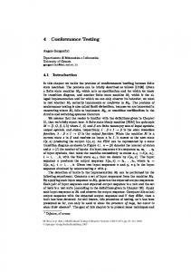
Abstract We present and compare different notions of conformance testing based on labeled transition systems. We formulate and prove several theorems which enable using synchronous conformance testing techniques such as input output conformance testing (ioco) in order to test implementations only accessible through asynchronous communication channels. These theorems define when the synchronous test cases are sufficient for checking all aspects of conformance that are observable by asynchronous interaction with the implementation under test. 1 Introduction Due to the ubiquitous presence of distributed systems (ranging from distributed embedded systems to the Internet), it becomes increasingly important to establish rigorous model-based testing techniques with an asynchronous model of communication in mind. This fact has been noted by the pioneering pieces of work in the area of formal conformance testing, e.g., see [8, Chapter 5], [11] and [12], and has been addressed extensively by several researchers in this field ever since [2, 5–7, 13, 14]. We stumbled upon this problem in our attempt to apply input-output conformance testing (ioco) [9, 10] to an industrial embedded system from the banking domain [1]. A schematic view of the implementation under test (IUT) and its environment is given in Figure 1.(a). The IUT is an Electronic Funds Transfer (EFT) switch (henceforth referred to as the switch), which provides a communication mechanism among different components of a card-based financial system. On one side of the IUT, there are components that the end-user deals with, such as Automated Teller Machines (ATMs), Point-of-Sale (POS) devices and e-Payment applications. On the other side, there are Core-Banking systems and the inter-bank network connecting the switches of different financial institutions. To test the switch, an automated on-line test-case generator is connected to it; the tester communicates (using an adapter) via a network with the IUT. This communication is inherently asynchronous and hence subtleties concerning asynchronous testing arise naturally in our context. A simplified specification of the switch, in which these subtleties appear, is depicted in Figure 1.(b). In this figure, the switch sends a purchase request to the core banking system and either receives a response, or after an internal step (e.g., an internal time-out, denoted by τ ) sends a reversal request to the POS. In the synchronous setting, after sending a purchase request and receiving a response, observing a reversal request will lead to the fail verdict. This is justified by the fact that receiving a response should force the system to take the topmost transition at the moment of choice in the specification depicted in Figure 1.(b). However, in the asynchronous
p rs? POS
Core Banking EFT
ATM
Switch
p rq!
(IUT) E-Payment
τ
Inter-bank Netw.
r rq!
(a)
(b)
Fig. 1 The EFT Switch and a simplified specification
setting, a response is put on a channel and is yet to be communicated to the IUT. It is unclear to the remote observer when the response is actually consumed by the IUT. Hence, even when a response is sent to the system the observer should still expect to receive a reversal request. The problems encountered in our practical case study have been encountered by other researchers. It is well-known that not all systems are amenable to asynchronous testing since they may feature phenomena (e.g., a choice between accepting input and generating output) that cannot be reliably observed in the asynchronous setting (e.g., due to unknown delays). In other words, to make sure that test-cases generated from the specification can test the IUT by asynchronous interactions and reach verdicts that are meaningful for the original IUT, either the class of IUTs, or the class of specifications, or the test-case generation algorithm (or a combination thereof) has to be adapted. Related work. In [13, Chapter 8] and [14], both the class of IUTs has been restricted (to the socalled internal choice specifications) and further the test-case generation algorithm is adapted to generate a restricted set of test-cases. Then, it is argued (with a proof sketch) that in this setting, the verdict obtained through asynchronous interaction with the system coincides with the verdict (using the same set of restricted test-cases) in the synchronous setting. We give a full proof of this result in Section 5 and report a slight adjustment to it, without which a counter-example is shown to violate the property. In [7] a method is presented for generating test-cases from the synchronous specification that are sound for the asynchronous implementation. The main idea is to saturate a test-case with observation delays caused by asynchronous interactions. In this paper, we adopt a restriction imposed on the implementation inspired by [7, Theorem 1] (dating back to [8]) and prove that in the setting of ioco testing this is sufficient for using synchronous test-case for the asynchronous implementation. In [5, 6] the asynchronous test framework is extended to the setting where separate testprocesses can observe input and output events and relative distinguishing power of these settings are compared. Although this framework may be natural in practice, we avoid following the framework of [5, 6] since our ultimate goal is to compare asynchronous testing with the standard ioco framework and the framework of [5, 6] is notationally very different. For the same reason, we do not consider the approach of [2], which uses a stamping mechanism attached to the IUT, thus observing the actual order input and output before being distorted by the queues. To summarize, the present paper re-visits the much studied issue of asynchronous testing and formulates and proves some theorems that show when it is (im)possible to synchronize asynchronous testing, i.e., interaction with an IUT through asynchronous channels and still obtain verdicts that coincide with that of testing the IUT using the synchronous interaction mechanisms. This paper substantially extends the results we reported in [3, 4]. Most importantly, we present a novel intensional representation of the conformance testing relation presented [13, 14] in this paper. (This was mentioned as future work in [3, 4].) Using this representation, we compare the testing power of different conformance relations in [10, 13, 14]. Moreover, we give external representations of the studied notions by providing a generic test-case generation algo2
rithm and show that the test case generation algorithm is sound and exhaustive with respect to our intensional representation. (The novel parts, compared to [3, 4], include the results presented in Sections 3 and 4.) Structure of the paper We present in Section 2 preliminary definitions regarding labeled transition systems and different variants thereof. In Section 3, we present a unifying intensional definition of input output conformance testing, from which the different conformance relations presented in [13, 14] and [10] can be obtained as special cases. In the same section, we define a notion of testing power and using that compare several notions of conformance relation obtained from different hypotheses assumed in [13, 14] and [10]. In Section 4, we present corresponding extensional notions of conformance testing using test cases and show that they are indeed sound and exhaustive with respect to their intensional counterparts. We give a full proof of the main result of [13, Chapter 8] and [14] (with a slight modification) in Section 5. Then, in Section 6, we re-formulate the same results in the pure ioco setting and show that our constraints precisely characterize the implementations for which asynchronous testing can be reduced to synchronous testing. The paper is concluded in Section 7.
2 Preliminaries In model-based testing theory, the two prevailing ways for modeling reactive systems are by using finite state machines (FSMs) [15] or labeled transition systems (LTSs) [10]. We are mainly concerned with the latter. In this section, we give a brief account of the concepts, relevant to LTS-based testing theory explored in this paper. LTS models consist of states and transitions. The latter are decorated with actions, modeling events that trigger state changes. Events that are internal to a system, i.e., unobservable to a tester or observer of the system, are modeled by the constant action τ . Definition 1 (LTS) A labeled transition system (LTS) is a 4-tuple hS, L, →, s0 i, where S is a set of states, L is a finite alphabet of actions that does not contain the internal action τ , →⊆ S × (L ∪ {τ }) × S is the transition relation, and s0 ∈ S is the initial state. We shall often refer to the LTS by referring to its initial state s0 . Fix an arbitrary LTS hS, L, →, s0 i. Let s, s0 ∈ S and x ∈ L∪{τ }. We use the standard notational x x x conventions, i.e., we write s −→ s0 rather than (s, x, s0 ) ∈→, we write s −→ when s −→ s0 x x for some s0 and we write s −→ X when not s −→. The transition relation is generalized to (weak) traces by the following deduction rules: σ
s =⇒ s00 �
s =⇒ s
x
s00 −→ s0
x 6= τ
σx
s =⇒ s0
σ
τ
s =⇒ s00 s00 −→ s0 σ s =⇒ s0
σ
σ
In line with our notation for transitions, we write s =⇒ if there is a s0 such that s =⇒ s0 , and σ σ s =⇒ X when no s0 exists such that s =⇒ s0 . Definition 2 (Traces and Enabled Actions) Let s ∈ S and S 0 ⊆ S. We define: S σ 1. traces(s) =def {σ ∈ L∗ | s =⇒}, and we define traces(S 0 ) =def s∈S 0 traces(s) S a 2. init(s) =def {a ∈ L ∪ {τ } | s −→}, and we define init(S 0 ) =def s∈S 0 init(s), S a 3. Sinit(s) =def {a ∈ L | s =⇒}, and we define Sinit(S 0 ) =def s∈S 0 Sinit(s).
A state in an LTS is said to diverge if it is the source of an infinite sequence of τ -labeled transitions. An LTS is divergent if one of its reachable states diverges. 3
Inputs, Outputs and Quiescence. In LTSs labels are treated uniformly. When engaging in an interaction with an actual system, the initiative to communicate is often not fully symmetric: the system is stimulated and observed. We therefore refine the LTS model to incorporate this distinction. Definition 3 (IOLTS) An input-output labeled transition system (IOLTS) is an LTS hS, L, → , s0 i, where the alphabet L is partitioned into a set LI of inputs and a set LU of outputs. Throughout this paper, whenever we are dealing with an IOLTS (or one of its refinements), we tacitly assume that the given alphabet L for the IOLTS is partitioned in sets LI and LU . In our examples we distinguish inputs from outputs by annotating them with a question- (?) and exclamation-mark (!), respectively. Note that these annotations are not part of action names. Observations of output, and the absence thereof, are essential ingredients in the conformance testing theories we consider. A system state that does not produce outputs is called quiescent. In its traditional phrasing, quiescence characterizes system states that do not produce outputs and which are stable, i.e., those that cannot evolve to another state by performing a silent action. Definition 4 (Quiescence and Outputs) State s ∈ S is called quiescent, denoted by δ(s), iff init(s) ⊆ LI . We say s is weakly quiescent, denoted by δq (s), iff Sinit(s) ⊆ LI . The outputs of S x s, denoted out(s) is the set {x ∈ LU | s −→} ∪ {δ | δ(s)}; we set out(S 0 ) = s0 ∈S 0 out(s0 ) The notion of weak quiescence is appropriate in the asynchronous setting, where the lags in the communication media interfere with the observation of quiescence: an observer cannot tell whether a system is engaged in some internal transitions or has come to a standstill. By the same token, in an asynchronous setting it becomes impossible to distinguish divergence from quiescence; we re-visit this issue in our proofs of synchronizing asynchronous conformance testing. We next recall the specialization of IOLTSs, introduced by Weiglhofer and Wotawa [13, 14]. Definition 5 (Internal choice IOLTS) An IOLTS hS, L, →, s0 i is an internal choice input output labeled transition system (IOLTSu ), if only quiescent states may accept inputs, i.e., for all s ∈ S, if init(s) ∩LI 6= ∅ then δ(s). We denote the class of IOLTSu models ranging over LI and LU by IOLTSu (LI , LU ). The Venn diagram below (which we extend in the next section) illustrates the relation between IOLTSu and IOLTS.
IOLTSu (LI , LU )
IOLTS(LI , LU )
Example 1 The LTS depicted in Figure 1.(b) is an IOLTS, but it is not in the IOLTSu subset. Namely, the only input action, i.e., p rs, is enabled at a state where the internal action τ is also enabled and is hence, not quiescent. We finish this section with a generalization of the extended transition relation =⇒ to also include observations of quiescence, and we use this to define the notion of suspension traces. For a given set of states S of an arbitrary IOLTS with transition relation →⊆ S × (L ∪ {τ }) × S, we define =⇒δ ⊆ S × (L ∪ {δ})∗ × S, through the following set of deduction rules: σ
s =⇒δ s0 �
s =⇒δ s
δ(s0 )
σδ
σ
x
s =⇒δ s00
s00 =⇒ s0 σx
s =⇒δ s0
s =⇒δ s0
Henceforth, given an alphabet L, we write Lδ to denote the set L ∪ {δ}. 4
Definition 6 (Suspension traces and After) Let hS, L, →, s0 i be an IOLTS. Let s ∈ S be an arbitrary state, S 0 ⊆ S and σ ∈ L∗δ . σ
1. The set of suspension traces of s, denoted Straces(s) is the set {σ ∈ L∗δ | s =⇒δ }; we set S 0 Straces(S ) = s0 ∈S 0 Straces(s0 ) σ 2. The σ-reachable states of s, denoted s after σ is the set {s0 ∈ S | s =⇒δ s0 }; we set S S 0 after σ = s0 ∈S 0 s0 after σ. 3 Implementation Relations Several formal testing theories build on the assumption that the implementations can be modeled by a particular IOLTS; this assumption is part of the so-called testing hypothesis underlying the testing theory. Not all theories rely on the same assumptions. We introduce two models, viz., the input output transition systems, used in Tretmans’ testing theory [10] and the internal choice input output transition systems, introduced by Weiglhofer and Wotawa [13, 14]. Tretmans’ input-output transition systems, formally defined below, are basically plain IOLTSs with the additional assumption that inputs can always be accepted. Definition 7 (IOTS) A state s ∈ S in an IOLTS hS, L, →, s0 i is input-enabled, iff LI ⊆ Sinit(s). The IOLTS s0 is an input output transition system (IOTS), iff every state s ∈ S is input-enabled. The class of input output transition systems ranging over LI and LU is denoted by IOTS(LI , LU ). Weiglhofer and Wotawa’s internal choice input output transition systems relax Tretmans’ input-enabledness requirement; at the same time, however, they impose an additional restriction on the presence of inputs, which stems from the fact that their class of implementations specialize the IOLTSu class. Definition 8 (Internal choice IOTS) An IOLTSu hS, L, →, s0 i is an internal choice input output transition system (IOTSu ), iff every quiescent state is input-enabled, i.e., for all s ∈ S, if δ(s), then LI ⊆ Sinit(s). We denote the class of IOTSu models ranging over LI and LU by IOTSu (LI , LU ). The following Venn-diagram depicts the relation between the IOLTS, IOLTSu , IOTS and IOTSu models. IOLTSu (LI , LU ) IOTSu (LI , LU )
IOLTS(LI , LU ) IOTS(LI , LU )
Example 2 Consider four IOLTSs c0 , e0 , o0 and i0 in Figure 2. All of them model a coffee machine which, after receiving money (m), either refunds it (r), or after that the coffee button is pressed (b), produces coffee (c). In IOLTS c0 , after receiving money, there is a choice between input and output; the exact behavior modeled by the transition system is, arguably, awkward, as by pressing a button the refund of the money can be prevented. Although IOLTS e0 does not feature an immediate race between input and output actions, the possibility of output r can still be ruled out by providing input b. IOLTS o0 in Figure 2 models a malfunctioning coffee machine which, after pressing the coffee button, may or may not deliver coffee. IOLTS i0 does not contain this fault and can be considered a reasonable specification of a coffee machine. 5
o0
b?
m? i0 o1 o2
m?
m?
m?
τ
r!
e0
c0
o3
i1
m?
r!
b? c1 r!
e1
b?
c2
τ e2
c3 c!
r!
m?
τ
b?,m?
i2
b?,m?
b?
b?
i3
o4 τ
e3 o5
c!
c! o6
b? b?,m? b?,m?
i4 τ
c4
e4
e5
τ
b?,m?
i5
c! i6
Fig. 2 IOLTSs with different moments of choice
IOLTS c0 is not input enabled, and neither is e0 : for example after input m, neither of the two allow for input m any more. IOLTS o0 is not input-enabled either, because for example at state o5 it refuses to accept any input. The aforementioned IOLTSs can be made IOTSs by adding self-loops for all absent input transitions at each and every state. IOLTS i0 is input-enabled, however, and is thus an IOTS. Neither c0 , nor e0 belong to the class IOLTSu , whereas o0 and i0 do. Namely, in the two IOLTSs o0 and i0 , input actions are only enabled in states where no output or internal action is enabled. Additionally, both o0 and i0 belong to the class IOTSu . IOLTSu i0 is input-enabled and hence is also an IOTSu . IOLTSu o0 is input-enabled in all states but o4 and o5 and since these two states are not quiescent, it follows from Definition 8 that o0 is indeed an IOTSu . In formal testing, an implementation is said to be correct when its executions are as prescribed by its formal specification. By the testing hypothesis, we can assume that implementations (and their behaviors) can be modeled by a matching IOTS (or IOTSu ). This assumption allows one to formalize the notion of conformance. Tretmans formalized in [10] a family of conformance relations by parameterizing a single behavioral relation with a set of decorated traces. We generalize this conformance relation by parameterizing it with the behavioral models it assumes as implementations and specifications, leading to a family of conformance relations. a b Definition 9 (iocoa,b F ) Let a, b ∈ {u, } and let i0 be an IOT S , s0 an IOLT S , and F ⊆ ∗ Lδ . We say that implementation i0 is input-output conforming to specification s0 , denoted by i0 iocoa,b F s0 , iff
∀σ ∈ F : out(i0 after σ) ⊆ out(s0 after σ) Remark 1 Note that IOT S a = IOT S.
depicts the space character (i.e., a blank). That is, for a =
we have
If we assume that our implementations can be modeled as IOTSs, the family of conformance relations iocoF, reduces to the family of conformance relations iocoF , studied by Tretmans [10]. By assigning F to Straces(s0 ) for a given specification s0 , the conformance relation ioco [10] is obtained. In the remainder of this section, we investigate several instances of the iocoa,b F testing theory. First, we study whether restricting the class of specifications in the iocoa,b relation affects the F testing power. Then, we consider how, for fixed specifications, the testing power of iocoa,b F is affected by considering different instances for F. We start by defining what it means for two classes of specifications to have equal testing power. 6
Definition 10 Let MODi be a class of implementations and let MODs be a class of specifications. Let MOD0s be a subset of the class of specifications MODs . Then MODs and MOD0s have the same testing power with respect to a given implementation relation imp : MOD × MODi , iff ∀s ∈ MODs : ∃s0 ∈ MOD0s : ∀i ∈ MODi : i impl s iff i impl s0 Informally, given a class of specifications MODs , a subclass MOD0s has equivalent testing power when for every specification from MODs , we can find an alternative specification from MOD0s that identifies exactly the same set of correct and the same set of incorrect implementations. Note that we do not require such an alternative specification to be obtained constructively. The theorem below states that restricting specifications from IOLTS to IOLTSu does influ, , i.e., ioco. ence the testing power with respect to implementation relation iocoStraces(s) Theorem 1 The testing power of IOLTSu is not equal to the testing power of IOLTS with respect , . to implementation relation iocoStraces(s) Proof Formally, we must show that the following statement does not hold: ∀s ∈ IOLTS(LI , LU ) : ∃s0 ∈ IOLTSu (LI , LU ) : , , ∀i ∈ IOTS(LI , LU ) : i iocoStraces(s) s iff i iocoStraces(s) s0 We will disprove this statement by showing that there is a specification in IOLTS whose testing power cannot be mimicked by any specification in IOLTSu . More specifically, we will show that there is a set of implementations on which the IOLTS specification’s verdict will always differ from any candidate alternative IOLTSu specification.
τ x! x! a?
a?
a? x!
x!
x! a?
a?
a? y!
a?
a?
a?
a? x!
x! a?
s
a?
a?
i1
i2
i3
Fig. 3 An input-output labeled transition system specification and three implementations that together show that conformance testing using internal-choice input-output labeled transition system specifications does not have the same testing power as conformance testing using input-output labeled transition systems (Theorem 1).
Consider the specification s ∈ IOLTS({a}, {x, y}), depicted in Figure 3. Observe that Straces(s) = {�, xδ ∗ , aδ ∗ , axδ ∗ }. Next, consider the three implementations i1 , i2 and i3 , also depicted in Figure 3. We have: – i1 ioco s, as for all σ ∈ Straces(s), out(i1 after σ) ⊆ out(s after σ). – i2 ioco 6 s, as we have out(i2 after a) = {y}, whereas out(s after a) = {x}. – i3 ioco 6 s, as we have out(i3 after �) = {x, δ}, whereas out(s after a) = {x}. We next show that no IOLTSu specification leads to the same partitioning on the set of implementations {i1 , i2 , i3 }, and, therefore, also not on the entire set of implementations IOT S. We first show that any IOLTSu specification s0 that satisfies i1 ioco s0 must necessarily also satisfy either i2 ioco s0 or i3 ioco s0 . More formally, we show that: ∀s0 ∈ IOLTSu (LI , LU ) : i1 ioco s0 implies (i2 ioco s0 ) or (i3 ioco s0 ) 7
(*)
Let s0 be an arbitrary IOLTSu specification such that i1 ioco s0 . Now, assume that i2 ioco 6 s0 . 0 Towards a contradiction, assume that i3 ioco 6 s . We then have z ∈ out(i3 after σ) and z ∈ / out(s0 after σ) for some z and some σ ∈ Straces(s0 ). Observe that for all σ 0 ∈ Straces(s0 ) \ Straces(i3 ), we have out(i3 after σ 0 ) = ∅ ⊆ out(s0 after σ 0 ), so, necessarily, σ ∈ Straces(s0 ) ∩ Straces(i3 ). We have Straces(i3 ) = {�} ∪ δ + ∪ δ ∗ a+ ∪ δ ∗ a+ x{δ, a}∗ ∪ x{δ, a}∗ We next analyze each of these possibilities. – Case σ = �. Since i1 ioco s0 , we have x ∈ out(s0 after �). As out(i3 after �) = {δ, x} and x ∈ out(s0 after �), we have δ ∈ / out(s0 after �). But then a ∈ / Sinit(s0 ), since in s0 , 0 inputs are only allowed in quiescent states. This means that s cannot distinguish between i1 and i2 , contradicting i1 ioco s0 and i2 ioco 6 s0 . So σ 6= �. + – Case σ ∈ δ . Since after observing quiescence, we are necessarily in a quiescent state, we find that out(i3 after σ) = {δ} = out(s0 after σ). So σ 6∈ δ + . – Case σ ∈ δ ∗ a+ . Observe that since s0 is an IOLTSu , we have out(s0 after ρ δ a0 ρ0 ) = out(s0 after ρ a0 ρ0 ) for all inputs a0 . This means that we have out(s0 after σ) = out(s0 after σ 0 ), where σ 0 ∈ a+ is obtained from σ by removing all observations of δ. Since out(i3 after σ) = {x}, we must have x ∈ / out(s0 after σ). Since out(s0 after σ) = 0 0 0 out(s after σ ), we find that x ∈ / out(s after σ 0 ). But that contradicts i1 ioco s0 . So ∗ + σ∈ /δ a . – Case σ ∈ δ ∗ a+ x{δ, a}∗ . We have out(i3 after σ) = {δ}, so, necessarily, δ ∈ / out(s0 after σ). Again, since s0 is an IOLTSu , we have out(s0 after σ) = out(s0 after σ 0 ), where σ 0 ∈ a+ xa+ is obtained from σ by removing all observations of δ. That means that δ ∈ / out(s0 after σ 0 ), which contradicts i1 ioco s0 . So σ ∈ / δ ∗ a+ x{δ, a}∗ . ∗ – Case σ ∈ x{δ, a} . Since out(i3 after σ) = {δ}, we must have δ ∈ / out(s0 after σ). Following the same reasoning as in the previous cases, we find that this contradicts i1 ioco s0 . So σ ∈ / x{δ, a}∗ . Since none of the possible traces σ ∈ Straces(i3 ) ∩ Straces(s0 ) can lead to out(i3 after σ) 6⊆ out(s0 after σ), we find that i3 ioco s0 . Summarizing, this means that there is no IOLTSu specification s0 that has the same testing power as the IOLTS specification s, proving Theorem 1. In the remainder of this section, we investigate the effect of varying the set of observations F on the testing power of the resulting conformance relations. Note that the question here is orthogonal to the one that we asked above: here we fix the specifications and ask whether by considering a subset of the set of observations F, we obtain conformance relations that retain the testing power of the full set of observations F. The proposition below states that the testing power of iocoa,b F is monotonic in the set of observations F; from this, it follows that testing power may be affected by considering different sets F. a,b Proposition 1 Let F, F 0 ⊆ L∗δ . Then F 0 ⊆ F implies iocoa,b F 0 ⊆ iocoF .
We are, in particular, interested in suspension traces that naturally capture the observations that we can make of an IOTSu implementation. The crucial difference between IOTSu implementations and IOTS implementations is that the latter are always willing to accept inputs, whereas the former only accepts inputs when we can also observe quiescence. Providing inputs in any other situation is undesirable, and, hence, reasoning about traces that would attempt to do so in our conformance relation would be equally undesirable. We therefore introduce a new class of traces, called internal choice traces, which naturally characterize the observable behaviors of IOTSu implementations. Definition 11 (Internal choice traces) Let hS, L, →, s0 i be an IOLTS. Let s ∈ S be an arbitrary state and σ ∈ L∗δ . The set of internal choice traces of s, denoted ICtraces(s) is a 8
subset of suspension traces in which quiescence is observed before every S input action, i.e. ICtraces(s) = Straces(s)∩(LU ∪({δ}+ LI )∪{δ})∗ ; we set ICtraces(S 0 ) = s0 ∈S 0 ICtraces(s0 ) for S 0 ⊆ S.
b? m? m?
b? r!
b?,m? t!
b?,m?
b?,m?
i Fig. 4 An implementation illustrating that the testing power of internal choice traces is strictly less than the testing power of suspension traces in the family of conformance relations iocoF .
Note that, as a result of Proposition 1, using internal choice traces instead of suspension traces leads to a weaker testing relation. It is not, however, immediate that the inclusion of Proposition 1 is strict. The following example shows that the inclusion is indeed strict in the standard ioco testing theory. Example 3 Let c0 be the specification depicted in Figure 2 and let i in Figure 4 be its implementation. Following Definition 9, i ioco 6 c0 because the observed output t in the implementation after execution of trace mb is not allowed by specification c0 after that trace. The set ICtraces(s) = {�, δσm, δσmr | σ ∈ δ ∗ }. Clearly, for all σ ∈ ICtraces(c0 ), we have out(i after σ) ⊆ out(c0 after σ). Hence, i iocoICtraces(c0 ) c0 . We next consider restricting the set of observations F to internal choice traces in the conformance family iocoF,u and compare the resulting testing power to the one obtained using suspension traces. As illustrated by example below, restricting the set of specifications to internal choice labeled transition systems is not a sufficient condition to retain the testing power of the full set of suspension traces. Example 4 Consider again Figure 2. Take IOLTSu o0 as specification and again consider i in Figure 4 as its implementation. Clearly, we have i ioco 6 o0 . For instance, considering trace mb, we find that out(i after mb) = {t}, whereas out(o0 after mb) = {c}. In conformance testing with respect to iocoICtraces(o0 ) , trace δmδb is examined instead of trace mb. We find that out(i after δmδb) = ∅ ⊆ out(o0 after δmδb). It is obtained by checking all other traces in ,u ICtraces(o0 ) that i iocoICtraces(o o0 . 0) We next investigate whether switching to a different model of implementations will change these results: we henceforth assume that implementations can be modeled using IOTSu s. The example below shows that, assuming that specifications can still be arbitrary IOLT Ss, the testing power of using internal choice traces is inferior to using suspension traces. Example 5 Consider IOLTS s in Figure 5. Analogous to the IOLTSs in Figure 2, it models a coffee machine which after receiving money, either refunds or accepts it; if accepted, coffee is produced after pressing a coffee button (in this case, cb ), and, similarly, tea is produced after pressing a tea button (tb ). The transition system i is input-enabled only at quiescent states, i.e., it is an IOTSu . Take IOTSu i, also in Figure 5, as a potential implementation. Regarding Definition 9, we find that i ioco 6 u s, because specification s after executing trace mcb allows only output c, whereas i after the same trace produces t. The set 9
m? m? τ r! τ r! tb ?
cb ? tb ?, cb ?
tb ?, cb ? c!
t! t! tb ?, cb ?
s
i
Fig. 5 A specification and an implementation illustrating that the testing power of internal choice traces is strictly less than the testing power of suspension traces in the family of conformance relations iocou, F .
ICtraces(s) = {�, σδm, σδmrσ, σδmcb cσ, σδmσδtb , σδmσδtb tσ | σ ∈ δ ∗ }. Obviously, we have out(i after σ) ⊆ out(s after σ). Hence, i iocou, ICtraces(s) s. Finally, we investigate the case that specifications are assumed to be internal choice IOLTSs. The result below shows that, contrary to the previous cases we analyzed, the resulting conformance relations for internal choice traces and suspension traces coincide. Theorem 2 Let s ∈ IOLTSu (LI , LU ) be a specification and i ∈ IOTSu (LI , LU ) be an impleu,u u,u mentation. Then i iocoICtraces(s) s iff i iocoStraces(s) s. Proof The implication from right to left is an instance of Proposition 1. We therefore focus on the implication from left to right. We first show that for every σ ∈ Straces(s), there is some σ 0 ∈ ICtraces(s) such that both s after σ = s after σ 0 and i after σ = i after σ 0 . We do this by induction on the number of input actions in σ. – Base case. For the induction basis assume that σ ∈ (LU ∪ {δ})∗ . Following Definition 11, σ ∈ ICtraces(s). Hence, σ 0 = σ satisfies the required condition. – Induction step. Assume for the induction step that the given claim holds for all sequences with n − 1 input actions. Suppose that we have a sequence σ with n input actions; that is, σ = σ1 aσ2 with σ1 ∈ L∗δ , σ2 ∈ (LU ∪ {δ})∗ and a ∈ LI . Thus, σ1 has n − 1 input actions. Following the induction hypothesis, there exists a σ10 ∈ ICtraces(s) such that s after σ1 = s after σ10 and i after σ1 = i after σ10 hold. We conclude from s ∈ IOLTSu (LI , LU ) along with σ1 a ∈ Straces(s) that there exists a non-empty subset of states in s after σ1 consisting of quiescent states. Suppose S 0 is the largest possible set of quiescent states in s after σ1 . We know from Definition 5 that s after σ1 aσ2 = S 0 after aσ2 . Consequently, by substituting S 0 with s after σ10 δ we have s after σ = s after σ10 δaσ2 . It follows from Definition 11 that σ10 δaσ2 ∈ ICtraces(s). Therefore, s after σ = s after σ10 δaσ2 holds. Along the same lines of reasoning, we can show that for the same internal choice trace we have i after σ = i after σ10 δaσ2 . u,u We next prove the property by contraposition. Suppose that i ioco 6 Straces(s) s. Then for some σ ∈ Straces(s), out(i after σ) 6⊆ out(s after σ). By the above result, we find that there must be some σ 0 ∈ ICtraces(s), such that i after σ = i after σ 0 and s after σ = s after σ 0 . But u,u then also out(i after σ 0 ) 6⊆ out(s after σ 0 ). So, it also must also hold that i ioco 6 ICtraces(s) s.
As an immediate consequence of Theorem 2, for implementations in the intersection of IOTSu and IOTS, the testing power of iocou,u ICtraces(s) and that of the standard ioco coincide, as stated by the proposition below. 10
Proposition 2 Let s ∈ IOLTSu (LI , LU ) be a specification and i ∈ IOTSu (LI , LU ) ∩ IOTS(LI , LU ) be an implementation. Then i iocou,u ICtraces(s) s iff i ioco s. 4 Test Case Generation The definition of the family of conformance relations introduced and studied in the previous section assumes that we can reason about implementations as if these were transition systems we can inspect. Since this is in practice not the case (we only know that a model exists that underlies such an implementation), the definition cannot be used to check whether an implementation conforms to a given specification. This problem can be sidestepped if there is a set of test cases that can be run against an actual implementation, and which has exactly the same discriminating power as the specification. In this section, we study the test cases that are needed to test for the family of conformance relations introduced in the previous section. A test case can, in the most general case, be described by a tree-shaped IOLTS. Such a test case prescribes when to stimulate an implementation-under-test by sending an input, and when to observe outputs emitted by the implementation-under-test. In general, the inputs to a test case are the outputs of the implementation-under-test, whereas the outputs of a test case are the inputs of the implementation-under-test. In order to formally distinguish between observing quiescence and “being” quiescent, we introduce a special action label θ, which stands for the former. Since we sometimes reason about the behaviors σ of an implementation from the viewpoint of a tester, we interpret δ labels as θ labels; formally, we then write σ to denote the sequence σ in which all δ labels have been replaced by θ labels. Definition 12 (Test case) A test case is an IOLTS hS, L, →, s0 i, in which: 1. S is a finite set of states reachable from s0 , 2. terminal nodes of S are called pass or fail, 3. the quiescence observation θ belongs to LI , 4. the transition relation → is acyclic, self-loop free and deterministic. 5. pass and fail states appear only as targets of transitions labeled by an element of LI , and 6. for all non-terminal states s, either init(s) = LI ∪ {θ} or init(s) = LI ∪ {x} for some x ∈ LU . We denote the class of test cases ranging over inputs LI and outputs LU by TTS(LU , LI ). Note that due to the determinism of a test case, none of the transitions of a test case are labeled with the silent action τ . In [14, 13] a subclass of TTS(LU , LI ) is introduced; test cases in this subclass are called internal choice test cases. Such test cases stimulate an implementation-under-test only when quiescence has been observed. Intuitively, this will ensure that the test case is actually executable for implementations that behave as internal choice transition systems. Definition 13 (Internal choice test case) A test case hS, L, →, s0 i is an internal choice test case, denoted TTSu , if for all s ∈ S, x ∈ LU and σ ∈ L∗ , if σx ∈ traces(s) then σ = σ 0 θ. We denote the class of internal choice test cases ranging over inputs LI and outputs LU by TTSu (LU , LI ). The property below provides us with an alternative characterization of an internal choice test case. Property 1 Let t be a test case. t is an internal choice test case iff traces(t) ⊆ (LU ∪({θ}+ LI )∪ {θ})∗ .
11
t0 θ
r?,c? fail
t1 r?,c? m! fail r?
t2 θ
t00 c?,r? m!
c?
pass
fail t4 c?,r? b!
r? pass
fail c?
t5
r?,θ
c?
pass
t01 c? b! t02
pass
fail
fail
fail r?,θ fail
t0
t Fig. 6 Two test cases for IOTSu o0 in Figure 2
Example 6 IOLTSs t and t0 in Figure 6 show two test cases for IOTSu o0 in Figure 2. IOLTS t0 is an internal choice test case. In this test case, inputs for the implementation are enabled only in states reached by a θ-transition. We next formalize what it means to execute a test case on an implementation-under-test. The intuition is that whenever a test case stimulates the implementation-under-test by sending an input, the latter consumes the input and responds by moving to a (possibly new) next state. In the same vein, whenever the implementation issues an output, the output is consumed by the test case, upon which the test case moves to a next state. Observe that the communication between the test case and the implementation-under-test can be instantaneous (i.e., synchronous), or through some underlying infrastructure that may introduce delays in the communication (i.e., communication is asynchronous). The latter form of communication is addressed in the next sections. In the remainder of this section, we assume that communication between implementations and test cases is synchronous. Definition 14 (Synchronous execution) Let hS, L, →, s0 i be an IOLTS, and let hT, L0 , →, t0 i be a test case, such that LI = L0U and LU = L0I \ {θ}. Let s, s0 ∈ S and t, t0 ∈ T . Then the synchronous execution of the test case and s0 is defined through the following inference rules: θ x x τ t −→ t0 δ(s) s −→ s0 t −→ t0 s −→ s0 τ
te|s −→ te|s0
(R1)
x
te|s −→ t0 e|s0
(R2)
(R3)
θ
te|s −→ t0 e|s
The terminal state(s) pass or fail of a test case can be used to formalize what it means for an implementation to pass or fail a test case. Definition 15 (Verdict) Let T ⊆ TTS(LI , LU ) be a set of test cases for some IOLTS implementation hS, L0 , →, s0 i and let t0 ∈ T be a test case. We say that state s ∈ S passes the test case σ t0 , denoted s passes t0 iff there is no σ ∈ L∗ and no state s0 ∈ S, such that t0 e|s0 =⇒ faile|s0 . We also say that state s ∈ S passes the set of test cases T , denoted s passes T iff s passes all test cases in T . We next introduce a test case generation algorithm, based on Tretmans’ original algorithm [9], that is suited for testing against a conformance relation iocoa,b F . The set of test cases generated by this algorithm is both sound and exhaustive. Soundness basically means that, for a given specification, executing the test case on an implementation-under-test will not lead to a test failure if the implementation conforms to the specification. Exhaustiveness boils down to the ability of the algorithm to generate a test case that has the potential to detect a non-conforming implementation. 12
Definition 16 (Soundness and exhaustiveness) Let T ⊆ TTS(LI , LU ) be a set of test cases for IOLTS specification s0 . Then for an implementation relation imp, we say that T is sound =def ∀i : i imp s0 implies i passes T T is exhaustive =def ∀i : i imp s0 if i passes T Note that Tretmans’ original test case generation algorithm did not produce test cases that were input-enabled. However, this issue was addressed fairly recently in [10], in which the algorithm for (plain) ioco was made to generate test cases that, in all non-terminal states, are willing to accept all the outputs produced by an implementation. We have used the ideas of the latter algorithm and incorporated them in Tretmans’ original algorithm. In order to concisely describe the algorithm, we borrow Tretmans’ notation (see for instance [10]) for behavioral expressions using the operators ; , � and Σ. Such behavioral expressions represent transition systems. Informally, for an action label a (taken from some set of actions), and a behavioral expression B, the behavioral expression a; B denotes the transition system that starts with executing the a action, leading to a state that behaves as B. For a countable set of behavioral expressions B, the choice expression ΣB denotes the transition system that, from its initial state, can nondeterministically choose between all behaviors described by the expressions in B. The expression B1 �B2 , for behavioral expressions B1 and B2 , is used as an abbreviation for Σ{B1 , B2 }, i.e., it behaves either as B1 or B2 . Algorithm 1 Let IOLTS hS, L, →, s0 i be a specification, let S 0 ⊆ S, and let F ⊆ Straces(S 0 ); then a test case t ∈ TTS(LU , LI ∪ {θ}) is obtained by a finite number of recursive application of one of the following nondeterministic choices: t := t :=
pass Σ{¯ x; fail | x ∈ LU , x 6∈ out(S 0 ), � ∈ F } � Σ{¯ x; pass | x ∈ LU , x 6∈ out(S 0 ), � 6∈ F } � Σ{¯ x; tx | x ∈ LU , x ∈ out(S 0 )}, where tx is obtained by recursively applying the algorithm for {σ ∈ L∗δ | xσ ∈ F } and S 0 after x � a; ta , where a ∈ LI , such that F 0 = {σ ∈ L∗δ | aσ ∈ F } = 6 ∅ and ta is obtained by recursively applying the algorithm for F 0 and S 0 after a t := Σ{¯ x; fail | x ∈ LU ∪ {δ}, x 6∈ out(S 0 ), � ∈ F } � Σ{¯ x; pass | x ∈ LU ∪ {δ}, x 6∈ out(S 0 ), � 6∈ F } � Σ{¯ x; tx | x ∈ LU ∪ {δ}, x ∈ out(S 0 )}, where tx is obtained by recursively applying the algorithm for {σ ∈ L∗δ | xσ ∈ F } and S 0 after x
Upon termination, algorithm 1 generates a test case for a set of states S 0 and a subset of its suspension traces F of a given specification s0 ∈ IOLTS(LI , Lu ). The parameters S 0 and F are typically initialized as s0 after � and Straces(s0 after �), respectively. The proposition below establishes a formal connection between a subset of the suspension traces of a given specification, and the traces of the test cases generated with Algorithm 1 for that specification. The proposition is essential in establishing the exhaustiveness of the test case generation algorithm. Proposition 3 Let hS, L, →, s0 i be an IOLTS. Let F ⊆ Straces(S 0 ) with S 0 ⊆ S, let σ ∈ F . Define t[σ,F,S 0 ] by: 13
t[�,F,S 0 ]
=def
Σ{¯ x; fail | x ∈ LU ∪ {δ}, x 6∈ out(S 0 )} � Σ{¯ x; pass | x ∈ LU ∪ {δ}, x ∈ out(S 0 )}
t[¯aσ,F,S 0 ] (¯ a ∈ LI )
=def
Σ{¯ x; fail | x ∈ LU , x 6∈ out(S 0 ), � ∈ F } � Σ{¯ x; pass | x ∈ LU , x 6∈ out(S 0 ), � 6∈ F } � Σ{¯ x; pass | x ∈ LU , x ∈ out(S 0 )} �a ¯; t[σ,F 0 ,S 00 ] (where F 0 = {σ 0 ∈ L∗δ | aσ 0 ∈ F } and S 00 = S 0 after a)
t[¯yσ,F,S 0 ] ] (¯ y ∈ LU ∪ {δ}) =def
Σ{¯ x; fail | x ∈ LU ∪ {δ}, x 6∈ out(S 0 ), � ∈ F } � Σ{¯ x; pass | x ∈ LU ∪ {δ}, x 6∈ out(S 0 ), � 6∈ F } � Σ{¯ x; pass | x ∈ LU ∪ {δ}, x ∈ out(S 0 ), x 6= y} � y¯; t[σ,F 0 ,S 00 ] (where F 0 = {σ 0 ∈ L∗δ | yσ 0 ∈ F } and S 00 = S 0 after y)
then 1. t[σ,F,S 0 ] can be obtained from F and S 0 with Algorithm 1 σx
2. x 6∈ out(S 0 after σ) implies t[σ,F,S 0 ] =⇒ fail Proof The proof is identical to the proof of Lemma A.25 in [10]. Theorem 3 Let IOLTS hS, L, →, s0 i be a specification. Then 1. a test case obtained with Algorithm 1 from s0 after � and F ⊆ Straces(s0 ) is sound for s0 with respect to iocoa,b F for a, b ∈ {u, }. 2. the set of all possible test cases that can be obtained from Algorithm 1 from s0 after � and F ⊆ Straces(s0 ) is exhaustive for s0 with respect to iocoa,b F for a, b ∈ {u, }. Proof The proof is similar to the proof of Theorem 6.3 in [10]; the exhaustiveness of the algorithm follows from Proposition 3. Observe that the above theorem does not imply that the test cases derived by Algorithm 1 can be executed successfully on both classes of implementations that we discussed in the previous sections. Whereas for Tretmans’ implementations behaving as IOTSs, successful test case execution is no issue, this is not the case for Weiglhofer and Wotawa’s implementations behaving as IOTSu s. For the latter class of implementations it is possible that the test case is forced to observe outputs, since the implementation is unwilling to accept stimuli from the test case. It thus makes no sense to consider such test cases, as the example below illustrates. Example 7 Consider again Figure 6. Take IOLTS t0 as the test case generated with Algorithm 1 from IOTS o0 and sequence m b and take IOTS d0 , depicted in Figure 7 as a potential implem mentation. Consider the execution t00 e|d0 −→ t01 e|d1 . At state t01 , test case t0 can try to provide the input b to the implementation-under-test while IOTS d0 is not willing to accept any inputs. Therefore, the test case is prevented from executing the sequence m b. To cope with the issue of successful executability of test cases, we next investigate when our test case generation algorithm can be made to produce only executable test cases, while still guaranteeing soundness and exhaustiveness. Our studies of the iocoa,b F family of conformance relations in the previous section are essential in establishing the latter results. First, we have the following technical lemma and proposition which state that traces of a test case can be chopped up into individual traces. 14
d0
b?
m?
r!
d1
d2 b?,m?
Fig. 7 An internal choice implementation of a malfunctioning coffee machine
Lemma 1 Let hS, L, →, s0 i be an IOLTS. Let S 0 ⊆ S be a set of states and F ⊆ Straces(S 0 ). Then for all yσ ∈ F we have: traces(t[yσ,F,S 0 ] ) = {�} ∪ LU ∪ {θ | y ∈ / LI } ∪ ({y} ∩ LI ) ∪ {yρ | ρ ∈ traces(t[σ,{ρ|yρ∈F },S 0 after y] )} Proof Follows immediately from the definition of traces(tσ,F,S 0 ). Proposition 4 Let hS, L, →, s0 i be an IOLTS. Let S 0 ⊆ S be a set of states and F ⊆ Straces(S 0 ). Then for all σ1 σ2 ∈ F satisfying σ1 6= �, we have: traces(t[σ1 σ2 ,F,S 0 ] ) = traces(t[σ1 ,F,S 0 ] ) ∪ {σ1 ρ | ρ ∈ traces(t[σ2 ,{ρ|σ1 ρ∈F },S 0 after σ1 ] )} Proof The proof proceeds by induction on the length of σ1 . – Base case. Follows immediately from Lemma 1. – Induction step. Assume for the induction step that the above statement holds for all sequences of length n − 1 and the length of σ1 is n. Suppose σ1 = xσ10 with σ10 ∈ L∗δ and x ∈ Lδ . Therefore, the length of σ10 is n − 1. From our base case we know that traces(t[xσ10 σ2 ,F,S 0 ] ) = traces(t[x,F,S 0 ] ) ∪ {xρ | ρ ∈ traces(t[σ10 σ2 ,F0 ,S0 ] )} where S0 = S 0 after x and F0 = {σ 0 | xσ 0 ∈ F }. Clearly, σ10 σ2 ∈ F0 . Following our induction hypothesis, traces(t[σ10 σ2 ,F0 ,S0 ] ) = traces(t[σ10 ,F0 ,S0 ] ) ∪ {σ10 ρ | ρ ∈ traces(t[σ2 ,F1 ,S1 ] )} where S1 = S0 after σ10 , F1 = {ρ | σ10 ρ ∈ F0 } and σ2 ∈ F1 . Combining these two observations results in: traces(t[xσ10 σ2 ,F,S 0 ] ) (*) = traces(t[x,F,S 0 ] ) ∪ {xρ | ρ ∈ traces(t[σ10 ,F0 ,S0 ] )} ∪ {σ10 ρ | ρ ∈ traces(t[σ2 ,F1 ,S1 ] )} From our base case, we know that: traces(t[xσ10 ,F,S 0 ] ) = traces(t[x,F,S 0 ] ) ∪ {xρ | ρ ∈ traces(t[σ10 ,F0 ,S0 ] )}
(**)
Together, ∗ and ∗∗ yield the desired equivalence. The proposition given below formalizes that, indeed, the interaction between an internal choice test case and an IOLTS proceeds in an orchestrated fashion: the IOLTS is only provided a stimulus whenever it has reached a stable situation, and is thus capable of consuming the stimulus. Proposition 5 Let s0 be an arbitrary IOLTS and t0 be an internal choice test case. Let x ∈ LI . Then for all σ ∈ L∗δ , we have: σx
te|s =⇒ implies ∃σ 0 ∈ L∗ : σ = σ 0 θ 15
Due to the above results, we can thus guarantee that test cases are successfully executable on implementations that behave as IOTSu s. It thus suffices to investigate whether the test case generation algorithm can be made to generate internal choice test cases only. The proposition below confirms that this is indeed possible. This proposition relies on Property 1. Proposition 6 Let hS, L, →, s0 i be an IOLTS. Then for all S 0 ⊆ S, all F ⊆ ICtraces(S 0 ) and all σ ∈ F , the test case t[σ,F,S 0 ] is an internal choice test case. Proof Because of Property 1, it suffices to show that traces(t[σ,F,S 0 ] ) ⊆ (LU ∪ ({θ}+ LI ) ∪ {θ})∗ . We prove it by induction on the number of input actions in σ. – Base case. Assume for the basis of the induction that σ ∈ (LU ∪ {δ})∗ . We proceed by a second induction on the length of σ. – Base case. Suppose σ = � for the basis of the second induction. From Proposition 3, we can deduce that traces(t[�,F,S 0 ] ) = {�} ∪ LU ∪ {θ}: t[�,F,S 0 ] has an x-labeled transition to the pass state for x ∈ out(S 0 ), and to the fail state for x ∈ / out(S 0 ). Clearly, + ∗ LU ∪ {θ} ∈ (LU ∪ ({θ} LI ) ∪ {θ}) . Hence, t[�,F,S 0 ] is an internal choice test case. – Induction step. Assume for the induction step of the second induction that the above statement holds for all sequences of length n − 1 and that the length of σ is n. Take σ = yσ 0 with σ ∈ (LU ∪ {δ})+ . Following Proposition 4, traces(t[yσ0 ,F,S 0 ] ) = {�} ∪ (LU ∪ {θ}) ∪ {¯ y ρ | ρ ∈ traces(t[σ0 ,F 0 ,S 00 ] )} with F 0 = {ρ | yρ ∈ F } and S 00 = S 0 after y. We know from our induction hypothesis that traces(t[σ0 ,F 0 ,S 00 ] ) ⊆ (LU ∪ ({θ}+ LI ) ∪ {θ})∗ . Consequently, we find that {¯ y ρ | ρ ∈ traces(t[xσ0 ,F 0 ,S 00 ] )} ⊆ (LU ∪ ({θ}+ LI ) ∪ ∗ {θ}) . Combined with our previous observations, we find that traces(t[σ,F,S 0 ] ) ⊆ (LU ∪ ({θ}+ LI ) ∪ {θ})∗ . – Induction step. Assume for the induction step that our statement holds for all sequences with n − 1 input actions. Let σ ∈ F be a sequence containing n input actions, where F ⊆ ICtraces(S 0 ); assume σ = σ1 δ a σ2 , where σ1 ∈ L∗δ , a ∈ LI and σ2 ∈ L∗U . From Proposition 4, we find that traces(t[σ,F,S 0 ] ) = traces(t[σ1 ,F,S 0 ] ) ∪ {σ1 ρ | ρ ∈ traces(t[δaσ2 ,F 0 ,S 00 ] )} where F 0 = {ρ | σ1 ρ ∈ F } and S 00 = S 0 after σ1 . From our induction hypothesis, we know that traces(t[σ1 ,F,S 0 ] ) ⊆ (LU ∪ ({θ}+ LI ) ∪ {θ})∗ . Therefore, it suffices to show that {σ1 ρ | ρ ∈ traces(t[δaσ2 ,F 0 ,S 00 ] )} ⊆ (LU ∪ ({θ}+ LI ) ∪ {θ})∗ . We know from σ1 ∈ ICtraces(S 0 ) that σ1 ⊆ (LU ∪ ((θ)+ LI ) ∪ {θ})∗ . Therefore, {σ1 ρ | ρ ∈ traces(t[δaσ2 ,F 0 ,S 00 ] )} ⊆ (LU ∪ ({θ}+ LI ) ∪ {θ})∗ follows if we can prove that traces(t[δaσ2 ,F 0 ,S 00 ] ) ⊆ (LU ∪ ({θ}+ LI ) ∪ {θ})∗ holds. By applying Proposition 4 twice, we find that traces(t[δaσ2 ,F 0 ,S 00 ] ) = traces(t[δ,F 0 ,S 00 ] ) ∪ traces(t[a,Fa0 ,Sa00 ] ) ∪ {δaρ | ρ ∈ traces(t[σ2 ,F 00 ,S 000 ] )} with Fa0 = {ρ | δρ ∈ F 0 }, F 00 = {ρ | δaρ ∈ F 0 }, Sa00 = S 00 after δ and S 000 = Sa00 after a. We know from Lemma 1 that traces(t[δ,F 0 ,S 00 ] ) = {�} ∪ LU ∪ {θ} and also traces(t[a,Fa0 ,Sa0 ] ) = {�} ∪ LU ∪ {a}. Following the base case of our induction, we find that traces(t[σ2 ,F 00 ,S 000 ] ) ⊆ (LU ∪ {θ})∗ as well. Combining all observations, we find that traces(t[δaσ2 ,F 0 ,S 00 ] ) = {�} ∪ LU ∪ {θ} ∪ {δx | x ∈ LU } ∪ {δa} ∪ {δaρ | ρ ∈ (LU ∪ {θ})∗ } From this, we obtain traces(t[δaσ2 ,F 0 ,S 00 ] ) ⊆ (LU ∪ ({θ}+ LI ) ∪ {θ})∗ , which was to be shown. Proposition 7 Let hS, L, →, s0 i be an IOLTS, let F ⊆ Straces(S 0 ) with S 0 ⊆ S, and let 0 T S be a set of test cases obtained with Algorithm 1 from S and F . We have traces(T ) ⊆ σ∈F traces(t[σ,F,S] ). 16
Proof The proof is given by induction on the number of recursions of Algorithm 1 in generating a test case t ∈ T . – Base case. We assume for the induction basis that test case t is generated by one time application of the algorithm. It is obvious that t := pass. It follows from traces(pass) = � that S traces(pass) ⊆ σ∈F traces(t[σ,F,S] ). – Induction step. For the induction basis assume that the above thesis holds for all test cases obtained from n − 1 times or less recursive application of the algorithm and test case t is generated from n times recursion. We distinguish two cases. – We suppose the second choice of the algorithm is selected at the first round of the application of the algorithm. Following the algorithm, traces(t) = {¯ x | x 6∈ S out(S)} x∈out(S) {¯ xρ | x ∈ out(S), ρ ∈ traces(tx )} ∪ {¯ aρ | a ∈ LI , ρ ∈ traces(ta )}. We consider three cases. • We consider x 6∈ out(S). Upon observing x 6∈ out(S), t goes to terminal states and the algorithm terminates. Therefore, t is obtained by one time application of the S algorithm. Following the induction hypothesis, {¯ x | x 6∈ out(S)} ⊆ σ∈F t[σ,F,S] . • We suppose that t := x; tx for some x ∈ out(S). We know that tx is obtained by recursively applying the algorithm for F 0 = {σ | xσ ∈ F } and S 0 = S after x. Clearly, tx is obtained by at most n − 1 times of application S of the algorithm. It follows from the induction hypothesis that traces(tx ) ⊆ σ∈F 0 traces(t[σ,F 0 ,S 0 ] ). We know from Lemma 1 that for every σ ∈ F 0 , {¯ xρ | ρ ∈ traces(t[σ,F 0 ,S 0 ] )} ⊆ {traces(t[xσ,F,S] )} (Note that ∀σ ∈ F 0 we know that xσ ∈ F S ). Therefore, the previous observation along with {¯ xρ | ρ ∈ S traces(tx )} ⊆ σ∈F 0 {xρ | traces(t[σ,F xρ | ρ ∈ traces(tSx )} ⊆ σ∈F traces(t[σ,F,S] ). ConseS 0 ,S 0 ] )} leads to {¯ quently, x∈out(S) {xρ | ρ ∈ traces(tx )} ⊆ σ∈F traces(t[σ,F,S] ) is resulted. • We suppose that t := a; ta for some a ∈ LI where F 0 = {σ | aσ ∈ F } = 6 ∅ and ta is obtained recursively by applying the algorithm for F 0 and S 0 = S after a. With the same S lines of reasoning in the previous item, we conclude that {aρ | ρ ∈ traces(ta )} ⊆ σ∈F traces(t[σ,F,S] ). S Therefore, we show that all three sets {¯ x | x 6∈ out(S)}, x∈out(S) {¯ xρ | x ∈ out(S), ρ ∈ traces(t )} and {¯ a ρ | a ∈ L , ρ ∈ traces(t )} are a subset of x I a S S traces(t ). Hence, traces(t) ⊆ traces(t ). [σ,F,S] [σ,F,S] σ∈F σ∈F – We suppose the third choice of the algorithm is selected at the first round of the application x | x 6∈ S of the algorithm. Following the algorithm, traces(t) = {¯ out(S)} x∈out(S) {¯ xρ | x ∈ out(S), ρ ∈ traces(tx )}. The remainder of the proof is identical to the previous one. Proposition 8 Let IOLTS s be a specification, let IOTSu i be an implementation, and let t be a test case generated with Algorithm 1 from s after � and ICtraces(s). Then t is an internal choice test case and hence, it is successfully executable against i. Proof We know from Propositions 6 and 7 that traces(t) ⊆ (LU ∪({θ}+ LI )∪{θ})∗ . Therefore, test case t is an internal choice test case. Following Proposition 5 i reaches a quiescent state before an input is provided by t; this input can be accepted by the implementation, which is input enabled in quiescent states. Therefore, t is executable against i. By combining Theorem 3 with the above proposition, we get the following corollary. It states that our test case generation algorithm is sound and exhaustive for the internal choice setting. Corollary 1 Let IOLTSu hS, L, →, s0 i be a specification. Then 1. a test case obtained with Algorithm 1 from s0 after � and ICtraces(s0 ) is sound for s0 with u,u respect to iocoICtraces(s . 0) 2. the set of all possible test cases that can be obtained from Algorithm 1 from s0 after � and ICtraces(s0 ) is exhaustive for s0 with respect to iocou,u ICtraces(s0 ) . 17
5 Adapting IOCO to Asynchronous Setting In order to perform conformance testing in the asynchronous setting in [13] and [14] both the class of implementations and test cases are restricted to internal choice class. Then, it is argued (with a proof sketch) that in this setting, the verdict obtained through asynchronous interaction with the system coincides with the verdict (using the same set of restricted test-cases) in the synchronous setting. In this section, we re-visit the approach of [13] and [14], give full proof of their main result and point out a slight imprecision in it.
5.1 Asynchronous Test Execution Asynchronous communication delays obscure the observation of the tester; for example, the tester cannot precisely establish when the input sent to the system is actually consumed by it. Asynchronous communication, as described in [8, Chapter 5], can be simulated by modelling the communications with the implementation through two dedicated FIFO channels. One is used for sending the inputs to the implementation, whereas the other is used to queue the outputs produced by the implementation. We assume that the channels are unbounded. By adding channels to an implementation, its visible behavior changes. This is formalized below. Definition 17 (Queue operator) Let hS, L, →, s0 i be an arbitrary IOLTS, σi ∈ L∗I , σu ∈ L∗U and s, s0 ∈ S. The unary queue operator [σu � �σi ] is then defined by the following axioms and inference rules: a
−→ [σu � s�σi a] , x [xσu � s�σi ] −→ [σu � s�σi ] , [σu � s�σi ]
a ∈ LI x ∈ LU
(A1) (A2)
τ
s −→ s0 τ 0 [σu � s�σi ] −→ [σu � s �σi ] a
s −→ s0 [σu � s�aσi ]
−→ [σu � s0 �σi ]
x
s −→ s0 [σu � s�σi ]
a ∈ LI τ
x ∈ LU
τ
−→ [σu x� s0 �σi ]
(I1)
(I2)
(I3)
We abbreviate [� � s�� ] to Q(s). Given an IOLTS s0 , the initial state of s0 in queue context is given by Q(s0 ). Observe that for an arbitrary IOLTS s0 , Q(s0 ) is again an IOLTS. We have the following property, relating the traces of an IOLTS to the traces it has in the queued context. σ
Property 2 Let hS, L, →, s0 i be an arbitrary IOLTS. Then for all s, s0 ∈ S, we have s =⇒ s0 σ implies Q(s) =⇒ Q(s0 ). The possibility of internal transitions is not observable to the remote asynchronous observer and hence, in [13, 14], weak quiescence is adopted to denote quiescence in the queue context. Definition 18 (Synchronous execution in the queue context) Let hS, L, →, s0 i be an IOLTS, and let hT, L0 , →, t0 i be a test case, such that LI = L0U and LU = L0I \ {θ}. Let s, s0 ∈ S and t, t0 ∈ T . Then the synchronous execution of the test case and Q(s0 ) is defined through the following inference rules: 18
[σu � s�σi ]
τ
−→ [σu0 � s0 �σi0 ] τ
te|[σu � s�σi ] −→ te|[σu0 � s0 �σi0 ] x
t −→ t0
[σu � s�σi ]
(R1’)
x
−→ [σu0 � s0 �σi0 ]
x
te|[σu � s�σi ] −→ t0 e|[σu0 � s0 �σi0 ] θ
t −→ t0
δq ([σu � s�σi ] )
(R2’)
(R3’)
θ
te|[σu � s�σi ] −→ t0 e|[σu � s�σi ] The property below characterizes the relation between the test runs obtained by executing an internal choice test case in the synchronous setting and by executing a test case in the queued setting. Property 3 Let hS, L, →, s0 i be an IOLTS and let hT, L0 , →, t0 i be a TTSu . Consider arbitrary states s, s0 ∈ S and t, t0 ∈ T and an arbitrary test run σ ∈ L0∗ . We have the following properties: σ
σ
1. te|s =⇒ t0 e|s0 implies te|Q(s) =⇒ t0 e|Q(s0 ) 2. Sinit(te|s) = Sinit(te|Q(s)). The proposition below proves to be essential in establishing the correctness of our main results in the remainder of Section 5. It essentially establishes the links between the internal behaviors of an implementation in the synchronous and the asynchronous settings. Proposition 9 Let hS, L, →, s0 i be an IOLTS and let hT, L0 , →, t0 i be a TTSu . For all states t ∈ T , s, s0 ∈ S, all σi ∈ L∗I and σu ∈ L∗U , we have: �
�
�
�
1. s =⇒ s0 iff te|s =⇒ te|s0 (R1∗ ) � � 2. [σu � s�σi ] =⇒ [σu � s0 �σi ] iff s =⇒ s0 (I1∗ ). Proof 1. s =⇒ s0 iff te|s =⇒ te|s0 (R1∗ ) � We prove the two implications by induction on the length of the τ -traces leading to =⇒: � 0 ⇒ Assume, for the induction basis, that i =⇒ i is due to a τ -trace of length 0; thus, i = i0 � � and it then follows that te|i =⇒ te|i and since i = i0 , we have that te|i =⇒ te|i0 , which was to be shown. � For the induction step, assume that the thesis holds for all =⇒ resulting from a τ -trace τ τ τ 0 of length n − 1 or less and that i −→ . . . −→ in−1 −→ i . It follows from the induc� τ tion hypothesis that te|i =⇒ te|in−1 . Also from in−1 −→ i0 and deduction rule R1 in � � Definition 14, we have that te|in−1 =⇒ te|i0 . Hence, that te|i =⇒ te|i0 , which was to be shown. ⇐ Almost identical to above. The induction basis is identical to the proof of the implication � from left to right. For the induction step, note that the last τ -step of te|in−1 =⇒ te|i0 can � only be due to deduction rule R1 and hence we have in−1 =⇒ i0 , which in turn implies � 0 that i =⇒ i . � � 2. [σu � i�σi ] =⇒ [σu � i0 �σi ] iff i =⇒ i0 (I1∗ ). Almost identical to the previous item: we prove � the two implications by induction on the length of the τ -trace for leading to =⇒: � ⇒ Assume, for the induction basis, that i =⇒ i0 is due to a τ -trace of length 0; thus, that � i = i0 . It then follows that [σu � i�σi ] =⇒ [σu � i�σi ] and since i = i0 , we have that � 0 [σu � i�σi ] =⇒ [σu � i �σi ] , which was to be shown. 19
�
For the induction step, assume that the thesis holds for all =⇒ resulting from a τ -trace τ τ τ of length n − 1 or less and that i −→ . . . −→ in−1 −→ i0 . It follows from the induc� τ tion hypothesis that [σu � i�σi ] =⇒ [σu � in−1 �σi ] . Also from in−1 −→ i0 and deduction rule I1 in Definition 17, we have that �
[σu � in−1 �σi ]
τ
−→
0 [σu � i �σi ] .Hence,
that
0
[σu � i�σi ] =⇒ [σu � i �σi ] , which was to be shown. ⇐ Similar to the above item. The induction basis is identical. The induction step follows � from the same reasoning. Note that [σu � in−1 �σi ] =⇒ [σu � i0 �σi ] can only be proven using deduction rule I1 in Definition 17, because deduction rules I2 and I3 produce modified queues in their target of the conclusion. Hence, the premise of deduction rule τ I1 should hold and thus, in−1 −→ i0 . Hence, using the induction hypothesis we obtain � that i =⇒ i0 .
5.2 Sound Verdicts of Internal Choice Test Cases In [14, 7], it is argued that providing inputs to an IUT only after observing quiescence (i.e., in a stable state), eliminates the distortions in observable behavior, introduced by communicating to the IUT using queues. Hence, a subset of synchronous test-cases, namely those which only provide an input after observing quiescence, are safe for testing asynchronous systems. This is summarized in the following claim from [14, 13] (and paraphrased in [7]): Claim (Theorem 1 in [14]) Let s0 be an arbitrary IOTSu , and let hT, L, →, t0 i be a TTSu . Then s0 passes t0 iff Q(s0 ) passes t0 . In [7], the claim is taken for granted, and, unfortunately, in [14, 13] only a proof sketch is provided for the above claim; the proof sketch is rather informal and leaves some room for interpretation, as illustrated by the following excerpt: “...An implementation guarantees that it will not send any output before receiving an input after quiescence is observed...” As it turns out, the above result does not hold in its full generality, as illustrated by the following example. Example 8 Consider the internal choice test case with initial state t0 in Figure 6. Consider the implementation modeled by the IOTSu depicted in Figure 2, starting in state o0 . Clearly, we find that o0 passes t0 ; however, in the asynchronous setting, Q(oo ) passes t0 does not hold. This is due to the divergence in the implementation, which gives rise to an observation of quiescence in the queued context, but not so in the synchronous setting. The claim does hold for non-divergent internal choice implementations. Note that divergence is traditionally also excluded from testing theories such as ioco. In this sense, assuming nondivergence is no restriction. Apart from the following theorem, we tacitly assume in all our formal results to follow that the implementation IOLTSs are non-divergent. Theorem 4 Let hS, L, →, s0 i be an arbitrary IOTSu and let hT, L0 , →, t0 i be a TTSu . If s0 is non-divergent, then s0 passes t0 iff Q(s0 ) passes t0 . Given the pervasiveness of the original (non-)theorem, a formal correctness proof of our corrections to this theorem (i.e., our Theorem 4) is highly desirable. In the remainder of this section, we therefore give the main ingredients for establishing a full proof for Theorem 4. We start by establishing a formal correspondence between observations of quiescence in the synchronous setting and observations of weak quiescence in the asynchronous setting. Lemma 2 Let hS, L, →, s0 i be an IOTSu . Let s ∈ S be an arbitrary state. Then δq (Q(s)) � implies δ(s0 ) for some s0 ∈ S satisfying s =⇒ s0 . 20
�
Proof Assume, towards a contradiction, that for all s0 ∈ S such that s =⇒ s0 , it doesn’t hold δ(s0 ). Take the s0 with the largest empty trace (by counting the numbers of τ -labeled transitions). Such s0 must exist since otherwise, there must be a loop of τ -labeled transition which is opposed to the assumption that s doesn’t diverge. Since s0 is not quiescent, according to Definition 4, x x there exists an x ∈ Lu such that s0 −→. Hence, there must exist an s00 ∈ S such that s0 −→ s00 . � It follows from Proposition 9 and deduction rule I3 in Definition 17 that Q(s) =⇒ [x� s00 ��] and since the output queue is non-empty we can apply the deduction rule A2 on the target state x x and obtain [x� s00 ��] −→ Q(s00 ). Combining the two transition we obtain Q(s) =⇒ Q(s00 ). From the latter transition we can conclude that Q(s) is not quiescent which is contradictory to the statement. The above lemma guarantees that all stimuli provided by an TTSu are accepted by implementations that behave as some IOTSu , even when we adopt the asynchronous communication scheme between testers and the implementation. Following the above lemma, the proposition below states that every asynchronous test case execution can lead to a state in which both communication queues are empty. Proposition 10 Let hS, L, →, s0 i be an IOTSu , and let hT, L0 , →, t0 i be a TTSu . Assume arbitrary states t0 ∈ T and s, s0 ∈ S, and an arbitrary test run σ ∈ L0∗ . Then for all σi ∈ L∗I and σu ∈ L∗U : σ
σ
t0 e|Q(s) =⇒ t0 e|[σu � s0 �σi ] implies ∃s00 ∈ S : t0 e|Q(s) =⇒ t0 e|Q(s00 ) Before we address the proof of the above proposition, we first need to show the correctness of some auxiliary lemmata given bellow. The lemma below states that only at weakly quiescent states the input queue can grow. Lemma 3 Let hS, L, →, s0 i be an IOTSu , and let hT, L0 , →, t0 i be a TTSu . Let s, s0 ∈ S, a t, t0 ∈ T be arbitrary states and σu ∈ L∗U and σi ∈ L∗I and a ∈ LI . If te|[σu � s�σi ] =⇒ t0 e|[σu � s0 �σi a] , then δq ([σu � s0 �σi ] ). a
Proof Assume a ∈ LI and te|[σu � s�σi ] =⇒ t0 e|[σu � s0 �σi a] , we know there exists an s00 ∈ S � a � such that te|[σu � s�σi ] =⇒ te|[σu � s00 �σi ] −→ t0 e|[σu � s00 �σi a] =⇒ t0 e|[σu � s0 �σi a] . It fol� � � lows from Proposition 9(2) that s =⇒ s00 and also s00 =⇒ s0 . We thus find that s =⇒ s0 � and subsequently according to Proposition 9(2) we have [σu � s�σi ] =⇒ [σu � s0 �σi ] . The � former observation and Proposition 9(1) lead to te|[σu � s�σi ] =⇒ te|[σu � s0 �σi ] . Using deduction rule A1 in Definition 17 and applying deduction rule R2 in Definition 14 result a in te|[σu � s0 �σi ] =⇒ t0 e|[σu � s0 �σi a] . Hence, there is a trace starting from te|[σu � s�σi ] to a te|[σu � s0 �σi ] =⇒ t0 e|[σu � s0 �σi a] . It follows then from Definition 13 that δq ([σu � s0 �σi ] ) (since test case t only provides an input immediately after if it has observed quiescence), which was to be shown. We find that in executing an internal choice test case on an implementation behaving as an IOLTSu , the input and output queues cannot be non-empty simultaneously. This is formalized by the lemma below. Lemma 4 Let hS, L, →, s0 i be an IOTSu , and let hT, L0 , →, t0 i be a TTSu . Let s, s0 ∈ S, σ t, t0 ∈ T be arbitrary states. There is no trace σu ∈ L0∗ such that te|Q(s) =⇒ t0 e|[σu � s0 �σi ] and the input and output queues are both non-empty at the same time(σi 6= � ∧ σu 6= �). Proof Assume, towards a contradiction, that the following two statements hold: σ
1. te|Q(s) =⇒ t0 e|[σu � s0 �σi ] 2. σi 6= � ∧ σu 6= � 21
Since both σi and σu are non-empty, there must exist the largest prefix σ 0 of σ during which the two queues are never simultaneously non-empty, i.e., by observing a single action after σ 0 , both queues become non-empty for the first time. Hence, there exists σ 0 , σ 00 ∈ L0∗ as a prefix and postfix of σ respectively and y ∈ L0 . 1. σ = σ 0 yσ 00 σ0
2. there exist σi0 ∈ (LI )∗ , σu0 ∈ (LU )∗ such that te|Q(s) =⇒ t1 e|[σu0 � s1�σi0 ] (with t1 ∈ T and s1 ∈ S) and ((σu0 = � ∧ σi0 6= �) ∨ (σi0 = � ∧ σu0 6= �)) y 3. there exist σi00 ∈ (LI )∗ , σu00 ∈ (LU )∗ such that t1 e|[σu0 � s1�σi0 ] −→ t2 e|[σu00 � s2�σi00 ] (with t2 ∈ T and s2 ∈ S) ∧((σu0 = � ∧ σi0 6= � ∧ σu00 6= � ∧ σi00 = σi0 ) ∨ (σi0 = � ∧ σu0 6= � ∧ σi00 6= � ∧ σu00 = σu0 )) σ 00
4. t2 e|[σu00 � s2�σi00 ] =⇒ t0 e|[σu � s0 �σi ] Note that after σ 0 both input and output queues cannot be empty, since a single transition y only increases the size of one of the two queues (see rules A1 and I3 in Definition 17). Below, we distinguish two cases based on the status of the input queue after executing the trace σ 0 : either the input queue is empty (and the output queue is not), or the other way around. 1. Case σu0 = �. The only possible transition that can fill an output queue is due to the application of deduction rule I3 in Definition 17. Hence, there must exists some s2 and x ∈ LU τ τ such that [�� s1�σi0 ] −→ [x� s2�σi0 ] and subsequently, (t1 e|[�� s1�σi0 ] −→ t2 e|[x� s2�σi0 ] ) (thereby satisfying the third item with σu0 = � and σu00 = x). The former x-labeled transix tion can only be due to deduction rule I3 in Definition 17 and hence, we have s1 −→ s2 . However, it follows from σi0 6= � that there exists an a ∈ LI , sp ∈ S, a prefix σp0 of σ 0 σp0
a
and ρi ∈ L∗I such that σi0 = ρi a and te|Q(s) =⇒ t01 e|[�� sp �ρi ] =⇒ t1 e|[�� s1�σi0 ] . We x
have from Lemma 3 that δq ([�� s1�ρi ] ). Using deduction rule A2 on s1 −→ s2 , we ob� tain that [�� s1�ρi ] =⇒ [x� s2�ρi ] . Hence according to Definition 4, state [�� s1�ρi ] is not quiescent, which contradicts our observation that δq ([�� s1�ρi ] ). 2. Case σi0 = �. The only transition which allows for filling the input queue is due to the subsequent application of deduction rules R2 and A1. Hence, there exists an a ∈ LI , such a a that t1 e|[σu0 � s1��] −→ t2 e|[σu0 � s2�a] ) and [σu0 � s1��] −→ [σu0 � s2�a] (where the for0 00 mer satisfies the third item by taking σi = � and σi = a). It follows from Lemma 3 that δq ([σu0 � s2��] ). However since σu0 6= �, there exists a y ∈ LU and ρu ∈ L∗U , such y that σu0 = yρu and using deduction rule A2, we obtain that that [σu0 � s2��] −→ and thus, 0 � s2��] is not quiescent, which contradicts our earlier observation. [σu Finally, the lemma given below states that in a queue context, implementations that have a non-empty input queue are weakly quiescent. The correctness of the lemma follows from the two preceding lemmata. Lemma 5 Let hS, L, →, s0 i be an IOTSu , and let hT, L0 , →, t0 i be a TTSu . Let s, s0 ∈ S, σ t, t0 ∈ T be arbitrary states, σ ∈ L0∗ , σi ∈ L∗I and σu ∈ L∗U . If te|Q(s) =⇒ t0 e|[σu � s0 �σi ] and σi 6= � then δq (s0 ) and σu = �. Proof By lemma 4, we have that σu = �. Assume, towards a contradiction that there exists an x ∈ LU such that x ∈ Sinit(s0 ). Since x ∈ Sinit(s0 ), it follows from Definition 2(3) that there x exists an s00 ∈ S such that s0 =⇒ s00 . Since σi 6= � there exist σ 0 ∈ L0∗ , sp ∈ S, tp ∈ T , a ∈ LI , σ0
a
and ρi ∈ L∗I such that σi = ρi a and te|Q(s) =⇒ tp e|[�� sp �ρi ] =⇒ t0 e|[�� s0 �σi ] . Hence by Lemma 3, [�� s0 �ρi ] is quiescent, i.e., δq ([�� s0 �ρi ] ). � It follows from the assumption that [�� s0 �ρi ] =⇒ [x� s00 �ρi ] . Since the output queue is x non-empty we can apply deduction rule A2 on the target state and obtain [x� s00 �ρi ] −→ 22
x
00 [�� s �ρi ] .
Combining the two transitions, we obtain [�� s0 �ρi ] =⇒ [�� s00 �ρi ] . From the latter transition, we conclude that [�� s0 �ρi ] is not quiescent which is a contradiction.
We now are in a position to formally establish the correctness of Proposition 10. Proof (Proposition 10). We distinguish four cases based on the status of input and output queues. 1. Case σi = �, σu = �. By assuming s0 = s, the statement holds. 2. Case σi 6= �, σu 6= �. According to Lemma 4, no trace leads to this situation. 3. Case σi = 6 �, σu = �. We prove this case by an induction on the length of σi . Since σi 6= �, for the induction basis, the smallest possible length of σi is one. Thus there must be an x ∈ LI such that σi = x. From Lemma 5, we know that ∀y ∈ LU , y ∈ / Sinit(s0 ) 0 and since s doesn’t diverge, it must reach eventually a state such as i ∈ S which performs a transition other than an internal one, hence the only possible choice is an input transition. From Definition 8 we know that δ(i) and state i is input-enabled as well. Thus ∃i0 ∈ S : x i −→ i0 . Due to the subsequent application of deduction rules of I1 , I2 in Definition 17 and � R1 in Definition 14, transition t0 e|[�� s0 �x] =⇒ t0 e|Q(i0 ) is possible. By assuming s00 = i0 σ and combination of the latter transition and the assumption, we have te|Q(s) =⇒ t0 e|Q(s00 ) which was to be shown. For the induction step, assume that the statement holds for all non-empty input queues of length n − 1 or less and length n for σi . It follows from σi 6= � that there exists an a ∈ σ0
LI , σi0 ∈ LI ∗, σ 0 ∈ L0∗ and i0 ∈ S and tp ∈ T such that σi = σi0 a and te|Q(s) =⇒ a tp e|[�� i0 �σi0 ] =⇒ t0 e|[�� s0 �σi ] . It follows from the induction hypothesis that ∃i ∈ S : σ0
te|Q(s) =⇒ tp e|Q(i). Due to the application of deduction rule R2 in Definition 14 and a A1 in Definition17, we have tp e|Q(i) =⇒ t0 e|[�� i�a] . It follows from the induction basis a that ∃s00 ∈ S : tp e|Q(i) =⇒ t0 e|Q(s00 ). Combining both transitions leads to ∃s00 ∈ S : σ te|Q(s) =⇒ t0 e|Q(s00 ) which was to be shown. 4. Case σi = �, σu 6= �. We prove this case by an induction on the length of σu . Since σu 6= �, for the induction basis, the smallest possible length of σu is one. Thus, assume, for the induction basis, that there exists an x ∈ LU such that σu = x. The only possible transition that can fill the output queue is due to the application of deduction rule I3 in Definition 17. Hence, there must exist some s00 , q 00 ∈ S such that τ � 00 0 00 0 x� s �σ 0 ] . Combining both transitions, we find 0 � s �σ 0 ] −→ [σ 0 x� q [σu �σi0 ] =⇒ [σu u i i 00 0 � s �σ 0 ] [σu i
�
=⇒ [σu0 x� s0 �σi0 ] . It follows from the application of deduction rule R1∗ in Proposition 9 that the input queue at state [σu0 � s00 �σi0 ] must be empty since otherwise according to Lemma 5, s00 would be quiescent and could not produce any output. Thus σ0
�
there exist σ 0 ∈ L0∗ , σu0 ∈ L∗U and t0p ∈ T such that te|Q(s) =⇒ t0p e|[σu0 � s00 ��] =⇒ 0 σu
t0p e|[σu0 x� s0 ��] =⇒ t0 e|[x� s0 ��] and σ = σ 0 σu0 . Applying deduction rules R2 in Definition σ0
u 14 and A2 in Definition 17, we find t0p e|[σu0 � s00 ��] =⇒ t0 e|Q(s00 ) and subsequently we have
σ0
σ0
u te|Q(s) =⇒ t0p e|[σu0 � s00 ��] =⇒ t0 e|Q(s00 ) which was to be shown. For the induction step, assume that the thesis holds for all non-empty output queues with length n − 1 or less and length of σu is n. It follows from σu 6= � that there exist an x ∈ LU , σu0 ∈ L∗U , σ 0 ∈ L0∗ and tp ∈ T and q, q 0 ∈ S such that σu = σu0 x
σ0
σ 00
τ
u and te|Q(s) =⇒ tp e|[σu00 σu0 � q��] −→ tp e|[σu00 σu0 x� q 0 ��] =⇒ t0 e|[σu0 x� s0 ��] and σ = 0 00 σ σu . Applying deduction rule R2 in Definition 14 and A2 in Definition 17, we have
σ 00
u tp e|[σu00 σu0 � q��] =⇒ t0 e|[σu0 � q��] . Thus we can run the previous execution in a new or-
σ0
σ 00
τ
u der such as te|Q(s) =⇒ tp e|[σu00 σu0 � q��] =⇒ t0 e|[σu0 � q��] −→ t0 e|[σu0 x� s0 ��] . Hence we can reach a new state with the output length less than the length of σu by running the same
23
σ
execution and it follows from the induction hypothesis that ∃s00 ∈ S : te|Q(s) =⇒ t0 e|Q(s00 ) which was to be shown. � As a consequence of the above proposition, we find the following corollary. It states that each asynchronous test execution can be chopped into individual observations such that before and after each observation the communication queue is empty. Corollary 2 Let hS, L, →, s0 i be an IOTSu , and let hT, L0 , →, t0 i be a TTSu . Assume arbitrary σx states t0 ∈ T and s, s0 ∈ S, and an arbitrary test run σ ∈ L0∗ and x ∈ L0 . Then t0 e|Q(s) =⇒ σ x t0 e|Q(s0 ) implies ∃t00 ∈ T, s00 ∈ S : t0 e|Q(s) =⇒ t00 e|Q(s00 ) =⇒ t0 e|Q(s0 ). Moreover, if x = θ then δq (Q(s0 )). The lemma below establishes a correspondence between the test runs that can be executed in the asynchronous setting and those runs one would obtain in the synchronous setting. The lemma is basic to the correctness of our main results in this section. Lemma 6 Let hS, L, →, s0 i be an IOTSu , and let hT, L0 , →, t0 i be a TTSu . Let s, s0 ∈ S and σ t0 ∈ T be arbitrary states. Then, for all σ ∈ L0∗ , such that t0 e|Q(s) =⇒ t0 e|Q(s0 ), there is a 00 0 � 00 non-empty set S ⊆ {s ∈ S | s =⇒ s } such that �
1. {s00 ∈ S | δ(s00 ) ∧ s0 =⇒ s00 } ⊆ S if ∃σ 0 ∈ L0∗ : σ = σ 0 θ 2. s0 ∈ S if @σ 0 ∈ L0∗ : σ = σ 0 θ σ 3. ∀s00 ∈ S : t0 e|s =⇒ t0 e|s00 . Proof We prove this lemma by induction on the length of σ ∈ L0∗ . �
– Induction basis. Assume that the length of σ is 0, i.e., σ = �. Assume that t0 e|Q(s) =⇒ � � t0 e|Q(s0 ). By Proposition 9(2) we have s =⇒ s0 . Set S = {s00 | s0 =⇒ s00 }. Let s00 ∈ S � � be an arbitrary state. Proposition 9(1) leads to t0 e|s =⇒ t0 e|s0 and t0 e|s0 =⇒ t0 e|s00 ; by � 00 0 transitivity, we have the desired t0 e|s =⇒ t0 e|s . It is also clear that s ∈ S. We thus find that S meets the desired conditions. – Inductive step. Assume that the statement holds for all σ 0 of length at most n − 1. Suppose σ that the length of σ is n. Assume that t0 e|Q(s) =⇒ t0 e|Q(s0 ). By Corollary 2, there is 0∗ some sn−1 ∈ S, a tn−1 ∈ T and σn−1 ∈ L and x ∈ L0 , such that σ = σn−1 x and σn−1 x t0 e|Q(s) =⇒ tn−1 e|Q(sn−1 ) =⇒ t0 e|Q(s0 ). � By induction, there must be a set Sn−1 ⊆ {s00 ∈ S | sn−1 =⇒ s00 }, such that � 00 00 00 0 0∗ 1. {s ∈ S | δ(s ) ∧ sn−1 =⇒ s } ⊆ Sn−1 if ∃σ ∈ L : σ = σ 0 θ 2. sn−1 ∈ Sn−1 if @σ 0 ∈ L0∗ : σ = σ 0 θ σn−1 3. ∀s00 ∈ Sn−1 : t0 e|s =⇒ tn−1 e|s00 . We next distinguish three cases: x ∈ LI , x ∈ LU and x ∈ / LI ∪ LU . θ
1. Case x = θ. We thus find that tn−1 e|Q(sn−1 ) =⇒ tn e|Q(s0 ). As a result of Corollary 2, we have δq (s0 ). We then find as a result of Lemma 2, there must be some state s00 ∈ S � � � such that sn−1 =⇒ s0 =⇒ s00 and δ(s00 ). Consider the set Sn = {s00 ∈ S | δ(s00 )∧s0 =⇒ 00 s }. Let s00 be an arbitrary state in Sn . Distinguish between cases sn−1 ∈ / Sn−1 and sn−1 ∈ Sn−1 . In the case, sn−1 ∈ / Sn−1 , we know from the construction of Sn−1 that s00 ∈ Sn−1 � � � and s00 =⇒ s00 always holds. In the case sn−1 ∈ Sn−1 , we have that sn−1 =⇒ s0 =⇒ σn−1 � θ s00 . We thus find that ∀s00 ∈ Sn ∃¯ s ∈ Sn−1 : t0 e|s =⇒ tn−1 e|¯ s =⇒ tn−1 e|s00 −→ t0 e|s00 . σn−1 x 0 Thus Sn has the desired requirement that t0 e|s =⇒ t e|s00 for all s00 ∈ Sn . Also, {s00 ∈ � S | δ(s00 ) ∧ s0 =⇒ s00 } ⊆ Sn is concluded from construction of Sn . Hence, Sn satisfies all desired conditions. 24
2. Case x ∈ LI . By Property 5, we find that the last step in σn−1 must be θ. It follows from corollary 2 that Q(sn−1 ) is weakly quiescent and consequently δq (sn−1 ). By induction � we have that {s00 ∈ S | δ(s00 ) ∧ sn−1 =⇒ s00 } ⊆ Sn−1 . Consider the set Sn = {s00 ∈ � S | s0 =⇒ s00 }. x x Transition tn−1 e|Q(sn−1 ) =⇒ t0 e|Q(s0 ) implies that sn−1 =⇒ s0 . By Lemma 2 and � x Definition 8, we know that ∃¯ s ∈ S such that sn−1 =⇒ s¯ =⇒ s0 and δ(¯ s). From construction of Sn−1 , we know that s¯ is in Sn−1 . We thus have ∀s00 ∈ Sn ∃¯ s ∈ Sn−1 : σn−1 x s =⇒ t0 e|s00 . t0 e|s =⇒ tn−1 e|¯ It is clear form construction of Sn that s0 ∈ Sn as the required condition that s0 ∈ Sn if the last step of σ is not θ-labeled transition. We thus find that Sn fulfills all desired requirements. 3. Case x ∈ LU . Analogous to the previous case. We are now in a position to establish the correctness of Theorem 4. We provide the proof below: Proof (Theorem 4) We prove the theorem by contraposition. σ0
1. Case ⇒. Suppose not Q(s) passes t0 . By Definition 15 and Proposition 10, t0 e|Q(s) =⇒ faile|Q(s0 ), for some σ 0 ∈ L0∗ and s0 ∈ S. As a result of Lemma 6, there is a non-empty set σ0
�
S ⊆ {s00 ∈ S | s0 =⇒ s00 } such that for all s00 ∈ S, t0 e|s =⇒ faile|s00 , which was what we needed to prove. σ0
2. Case ⇐. Assume, that not s passes t0 . Then there are σ 0 ∈ L0∗ and s00 ∈ S, t0 e|s =⇒ σ0
faile|s00 . Using Property 3 leads to t0 e|Q(s) =⇒ faile|Q(s00 ).
6 Adapting Asynchronous Setting to IOCO In this section, we re-cast the results of the previous section to the setting with ioco test-cases. We first show that the result of Theorem 2 cannot be trivially generalized to the asynchronous setting. Then using an approach inspired by [8, Chapter 5] and [7], we show how to re-formulate Theorem 4 in this setting. In section 3 it is shown that restricting the set of traces F in implementation relation iocoa,b F will lead to a weaker testing power. Yet, we proved in Theorem 1 that discrimination power of iocoa,b Straces(s) for a given specification s does not decrease by examining internal choice traces of s instead of suspension traces in setting a, b ∈ {u}. But, in the following example, we motivate u,u that the testing power of iocou,u ICtraces(s) and iocoStraces(s) are different in the asynchronous setting. Example 9 IOLTS t0 in Figure 6 shows a test case for IOLTS o0 in Figure 2, which is an internal choice IOTS. Assume that at the same time o0 is also used as the implementation. For o0 as specification and implementation, we have that o0 ioco o0 . However, we can reach a fail verdict for o0 under the queue context when using the test case t00 . Consider the sequence m � � mbr ; in the queue context, the execution t00 e|Q(o0 ) −→ t01 e|[�� o0�m] =⇒ t01 e|Q(o1 ) =⇒ b
r
t01 e|[r � o2��] −→ t02 e|[r � o2�b] −→ faile|[�� o2�b] is possible, which leads to the fail state. Note that the fail verdict is reached even if we omit divergence from the implementation o0 . This shows that Theorem 4 cannot be trivially generalized to the ioco setting (even when excluding divergence and allowing for non-input-enabled states). Our main interest in this section is to investigate implementations for which ioco test cases cannot distinguish between synchronous and asynchronous modes of testing. To this end, we consider the relation between traces of a system and those of the system in queue context. 25
Definition 19 (Delay relation) Let L be a finite alphabet partitioned in LI and LU . The delay relation @⊆ L∗δ × L∗δ is defined by the following deduction rules:
σ@σ
ρi , σi ∈ L∗I σu ∈ L∗U PUSH ρi σu σi @ ρi σi σu
REF
σ @ σ0 ρ@ρ0 COM σρ @ σ 0 ρ0
Proposition 11 Let hS, L, →, s0 i be an IOTS. Let s ∈ S and σ ∈ L∗δ . Then σ ∈ Straces(Q(s)) implies there is a σ 0 ∈ Straces(s) such that σ 0 @ σ. Before we give the proof of the above proposition, we prove the lemmata given below. These allow us to establish links between traces in the synchronous and asynchronous settings. Lemma 7 Let hS, L, →, s0 i be an IOTS, s ∈ S and σ ∈ L∗δ . Then σ ∈ Straces(Q(s)) implies σ that there is a s0 ∈ S such that Q(s) =⇒δ Q(s0 ). Proof The proof is given by induction on the number of δ in σ ∈ L∗δ . – Induction basis: Assume the number of δ in σ is 0, i.e., σ ∈ L∗ . We distinguish between two cases based on whether σ ∈ L∗I and σ ∈ / L∗I . σ ∗ 1. Case σ ∈ LI : Due to deduction rule A1 in Definition 17, it always holds that Q(s) =⇒ σ 0 0 [�� s�σ] . Since s is input-enabled, there is a state s ∈ S such that s =⇒ s . By applying � deduction rule I2 several times, we have [�� s�σ] =⇒ Q(s0 ). We thus find that s0 meets the required condition. 2. Case σ ∈ / L∗I : Let σ = σ 0 xρ, with σ 0 ∈ L∗ , x ∈ LU and ρ ∈ L∗I . The appearance of x in 0 trace σ xρ can only be due to deduction rules I3 and A2 in Definition 17 and hence, we should have σ1 σ2 τ Q(s) =⇒ [σu � s1�σi ] −→ [σu x� s2�σi ] =⇒ [xσv � s3�σj ]
ρ
x
−→ [σv � s3�σj ] =⇒ [σw � s00 �σk ]
for σw , σu , σv ∈ L∗U , σk , σi , σj ∈ L∗I and s00 , s1 , s2 , s3 ∈ S. We conclude from the last observation and deduction rules A2 in Definition 17 that σu must be the projection of σ2 onto L∗U . It follows from the last observation and deduction rules A1 and A2 that σ2 xρ also the following derivation is possible, [σu x� s2�σi ] =⇒ [�� s2�σi σ20 ρ] , where σ20 is ∗ the projection of σ2 onto LI . Since, s2 is input-enabled there is a state s0 ∈ S such σi σ 0 ρ
σi σ 0 ρ
2 2 that s2 =⇒ s0 . By using deduction rule I2 , we have [�� s2�σi σ20 ρ] =⇒ Q(s0 ). Thus s0 meets the required condition. – Inductive step: Assume that the statement holds for all σ 0 ∈ L∗δ with at most n − 1 occurrences of δ. Suppose the number of occurrences of δ in σ is n. Since σ ∈ Straces(Q(s)), σ there exists a state s00 ∈ S such that Q(s) =⇒ [σu � s00 �σi ] for some σi ∈ L∗I and σu ∈ L∗U . Assume σ = σ1 δ¯ σ with σ1 ∈ L∗ and σ ¯ ∈ L∗δ . Due to Definition 6 the following step has to
σ δ
σ ¯
1 be taken in the former derivation, Q(s) =⇒ δ [σv � s1�σj ] =⇒δ , where δq ([σv � s1�σj ] ) for ∗ ∗ some s1 ∈ S ,σv ∈ LU and σj ∈ LI . Note that σv has to be empty since quiescence has been observed beforehand. It follows from Definition 4 that σj has to be empty as well, since otherwise, [σv � s1�σj ] can perform an internal transition, hence it cannot be quiescent. We
σ δ
σ ¯
1 thus find that Q(s) =⇒ δ Q(s1 ) =⇒δ and s1 is quiescent. We take the last transition of the previous derivation. It follows from the induction hypothesis that ∃s0 ∈ S such that σ ¯ Q(s1 ) =⇒δ Q(s0 ). We thus conclude from the last observation that there is a state s0 ∈ S
σ δ
σ ¯
1 0 such that Q(s) =⇒ δ Q(s1 ) =⇒δ Q(s ) which was to be shown.
σ
Lemma 8 Let hS, L, →, s0 i be an IOTS. Let s ∈ S and σ ∈ Straces(Q(s)). Then Q(s) =⇒ σ
0
Q(s0 ) implies there is a σ 0 ∈ Straces(s) such that s =⇒ s0 and σ 0 @ σ. 26
Proof The proof is given by induction on the number of δ in σ ∈ L∗δ . – Induction basis. Assume that there is no occurrence of δ, i.e., σ ∈ L∗ . Thus, the thesis reduces to σ ∈ Straces(Q(s)) and σ ∈ L∗ implies there is a σ 0 ∈ traces(s) such that σ 0 @ σ. We prove the latter by induction on the number of output actions in σ ∈ L∗ . – Induction basis. Assume the number of output actions in σ is 0, i.e., σ ∈ L∗I . By Propoσ sition 7, we have σ ∈ Straces(Q(s)), implying that ∃s0 ∈ S : Q(s) =⇒ Q(s0 ). This derivation can only be done by applying deduction rules A1, I2 and maybe I1 in Defiσ nition 17 some times which result in s =⇒ s0 and subsequently σ ∈ Straces(s). Using deduction rule REF in Definition 19 results in σ@σ. By assuming σ 0 = σ, it fulfills the two desired properties. – Inductive step. Assume that the statement holds for all σ 00 ∈ L∗ with at most n−1 output actions. Suppose that the number of output actions of σ is n. Assume that σ = ρx¯ σ with ρx¯ σ ρ ∈ L∗I , x ∈ LU and σ ¯ ∈ L∗ . We have Q(s) =⇒ Q(s0 ), implying that somewhere x in this derivation the step s1 −→ s2 is taken, for some s1 , s2 ∈ S. This implies that there are two prefixes ρ1 and ρ2 of ρ such that ρ2 is a prefix of ρ1 as well and also ρ1
τ
Q(s) =⇒ [�� s1�ρ1 \ρ2 ] −→ [x� s2�ρ1 \ρ2 ]
(ρ\ρ1 )x¯ σ
=⇒
Q(s0 ). The last step of the previous (ρ\ρ1 )¯ σ
derivation and deduction rule A2 in Definition 17 lead to [�� s2�ρ1 \ρ2 ] =⇒ Q(s0 ). Since the input queue can be filled only under deduction rule A1 in Definition 17 that (ρ1 \ρ2 )(ρ\ρ1 )¯ σ
σ
1 =⇒ Q(s0 ). By defining σ1 = (ρ \ ρ2 )¯ σ , we have Q(s2 ) =⇒ Q(s0 ) Q(s2 ) ∗ with σ1 ∈ L and one output action less than n. It follows from induction hypothesis
σ0
ρ2
x
σ0
1 1 that ∃σ10 ∈ Straces(s2 ) : s2 =⇒ s0 ∧ σ10 @σ1 . We thus have s =⇒ s1 −→ s2 =⇒ s0 0 and subsequently, ρ2 xσ1 ∈ Straces(s). By applying deduction rule REF and COM in Definition 19 respectively, we have xσ10 @x(ρ \ ρ2 )σ1 . On the other hand, due to rule REF and COM we know that x(ρ \ ρ2 )σ1 @(ρ \ ρ2 )xσ1 and consequently, xσ10 @(ρ \ ρ2 )xσ1 . Deduction rule COM , the last observation and ρ2 @ρ2 lead to ρ2 xσ10 @ρ2 (ρ \ ρ2 )xσ1 . By defining σ 0 = ρ2 xσ10 , we have σ 0 @ρ2 (ρ \ ρ2 )xσ 0 and more clearly, σ 0 @σ. We thus find that σ 0 meets the two desired conditions. – Inductive step. Assume the statement holds for all σ with at most n − 1 occurrences of δ. Suppose there are n occurrences of δ in σ. Assume σ = σ1 δ¯ σ with σ1 ∈ L∗ and σ ¯ ∈ L∗δ . 0 By Proposition 7, we know from σ ∈ Straces(s) that there is a state s ∈ S such that
σ δσ ¯
1 0 Q(s) =⇒ δ Q(s ). Due to Definition 4 and Definition 6, there exists a state s1 ∈ S such
σ δ
σ ¯
1 0 that Q(s) =⇒ δ Q(s1 ) =⇒δ Q(s ) and δ(s1 ). By taking the first transition of the previous
σ0
1 derivation and induction basis, we find that there exists σ10 ∈ Straces(s) such that s =⇒ s1
σ0 δ
1 and σ10 @σ. From δ(s1 ), we have s =⇒ δ δ s1 and consequently by applying deduction rule 0 COM in Definition 19, σ1 δ@σ1 δ is concluded. Take then, the last transition of the first σ ¯ derivation i.e, Q(s1 ) =⇒δ Q(s0 ) with σ ¯ ∈ L∗δ and the number of occurrences of δ is n − 1 (one less than σ). By our induction hypothesis we find that there exists a σ ¯ 0 ∈ Straces(s1 )
σ0 δ
σ ¯0
1 such that s1 =⇒δ s0 and σ ¯ 0 @¯ σ . We thus have ∃σ10 ∈ Straces(s), σ ¯ 0 ∈ Straces(s1 ) : s =⇒ δ
σ ¯0
s1 =⇒δ s0 . By applying deduction rule COM to the first and second observation, i.e., ¯ 0 @¯ σ , we have σ10 δ¯ σ 0 @σ1 δ¯ σ . By defining σ 0 = σ10 δ¯ σ 0 we find that σ 0 satisfies σ10 δ@σ1 δ and σ the two required properties. We are now in a position to prove the correctness of the Proposition 11 as given below. Proof Using the lemmata given above, the proof of the statement follows from the observations σ below. We have that σ ∈ Straces(Q(s)), implying that ∃s0 ∈ S : Q(s) =⇒ Q(s0 ), due to σ0
Lemma 7. It follows from the previous observation and Lemma 8 that ∃σ 0 ∈ Straces(s) : s =⇒ s0 and σ 0 @σ which was to be shown. 27
Definition 20 (Delay right-closed IOTS) Let hS, L, →, s0 i be an IOTS. A set L0 ⊆ L∗δ is delay right-closed iff for all σ ∈ L0 and σ 0 ∈ L∗δ , if σ @ σ 0 then σ 0 ∈ L0 . The IOTS s0 is delay right-closed iff Straces(s0 ) is delay right-closed. We denote the class of delay right-closed IOTSs ranging over LI and LU by IOTS@ (LI , LU ). The property below gives an alternative characterisation of delay right-closed IOTSs. Property 4 Let hI, L, →, i0 i be an IOTS. The IOTS i0 is delay right-closed if for all σ ∈ L∗δ , all x ∈ LU and a ∈ LI , we have: σxa ∈ Straces(i0 ) then σax ∈ Straces(i0 )
s0
p rs?
p rq!
p rq!
p rs?
s2
p rs?
s5
p rs?
s1
τ p rs?
p rs? s3
s4
p rs?
r rq!
r rq! s7
p rs?
s6
p rs?
Fig. 8 A delay right-closed IOTS
Example 10 Consider the IOTS s0 given in Figure 8. It is not hard to check that s0 is delay right-closed. As stated in the following theorem, the verdicts obtained by executing an arbitrary test case on a delay right-closed IOTS do not depend on the execution context. That is, the verdict does not change when the communication between the implementation and the test case is synchronous or asynchronous. Theorem 5 Let hI, L, →, i0 i be a delay right-closed IOTS and let hT, L0 , →, t0 i be an arbitrary test case. Then i0 passes t0 iff Q(i0 ) passes t0 . Before we address the proof of the above theorem, we first establish the correctness of the lemma below, stating that the suspension traces of a delay right-closed IOTS, as observed in an asynchronous setting are indistinguishable from the set of suspension traces observable in the synchronous setting. Lemma 9 Let hS, L, →, s0 i be a delay right-closed IOTS. Then Straces(Q(s0 )) = Straces(s0 ). Proof We divide the proof obligation into two parts: Straces(Q(s0 )) ⊆ Straces(s0 ) and Straces(s0 ) ⊆ Straces(Q(s0 )). It is not hard to verify that the latter holds vacuously, even for arbitrary IOTSs. It therefore remains to show that Straces(Q(s0 )) ⊆ Straces(s0 ). Consider a σ ∈ Straces(Q(s0 )); by Proposition 11, ∃σ 0 ∈ Straces(s0 ) : σ 0 @ σ. As s0 is delay right-closed, we obtain the required σ ∈ Straces(s0 ). The above lemma is at the basis of the correctness of Theorem 5. Proof (Theorem 5) Using the lemma given above, the proof of the theorem follows from the observation that for all test cases hT, L0 , →, t0 i and all σ ∈ L0∗ : σ
∃i0 ∈ I : t0 e|i0 =⇒ faile|i0 iff σ
∃i0 ∈ I, σi ∈ L∗I , σu ∈ L∗U : t0 e|Q(i0 ) =⇒ faile|[σu � i0 �σi ] 28
Theorem 6 Let hI, L, →, i0 i be a delay right-closed IOTS and let IOLTS hS, L, →, s0 i be a specification. Then i0 ioco s0 iff Q(i0 ) ioco s0 . Proof Follows from the existence of a sound and complete test suite that can test for ioco, and the proof of Theorem 5. We now show that delayed right-closedness of implementations is also a necessary condition to ensure the same verdict in the synchronous and the asynchronous setting. Theorem 7 Let hI, L, →, i0 i be an IOTS. If for every test case hT, L0 , →, t0 i, we have i0 passes t0 ⇔ Q(i0 ) passes t0 , then i0 is a delay right-closed IOTS. Proof We prove the theorem by contraposition, i.e., we show that if we test a non-delay rightclosed IOTS, there is a test case that can detect this by giving a pass verdict in the synchronous setting but a fail verdict in the asynchronous setting. Let hI, L, →, i0 i be an IOTS that is not delay right-closed. Thus, there is some x ∈ LU , a ∈ LI such that σxa ∈ Straces(i0 ), but not σax ∈ Straces(i0 ). Let hT, L0 , →, t0 i be a test case such that there is a t0 ∈ T satisfying: σ
1. t0 =⇒ t0 , a x 2. t0 −→ t00 , and t00 −→ fail. σ0 3. for all σ 0 such that t0 =⇒ fail we have σ 0 = σax. Observe that the existence of such a test case is immediate. Then there are σi ∈ L∗I , σu ∈ L∗U σax and a state i ∈ (i0 after σ) such that t0 e|Q(i0 ) =⇒ faile|[σu � i�σi a] , i.e., not Q(i0 ) passes t0 . σax However, we do not have t0 e|i0 =⇒ faile|i. By construction of the test case, we find that i0 passes t0 .
7 Conclusions In this paper, we studied the theoretical foundations for synchronous and asynchronous conformance testing. To this end, we gave unifying intensional and extensional definitions of conformance testing relations and compared them extensively. Subsequently, we presented theorems which allow for using test-cases generated from ordinary specifications in order to test asynchronous systems. These theorems establish sufficient conditions when the verdict reached by testing the asynchronous system (remotely, through FIFO channels) corresponds with the local testing through synchronous interaction. In the case of ioco testing theory, we show that the presented sufficient conditions are also necessary. The presented conditions for synchronizing ioco are semantic in nature and we intend to formulate syntactic conditions that imply the semantic conditions presented in this paper. For example, it is interesting to find out which composition of programming constructs and / or patterns of interaction satisfy the constraints established in this paper. The research reported in this paper is inspired by our practical experience with testing asynchronous systems reported in [1]. We plan to apply the insights obtained from this theoretical study to our practical cases and find out to what extent the constraints of this paper apply to the implementation of our case studies. Acknowledgments. We would like to thank Sjoerd Cranen (TU/e) and Maciej Gazda (TU/e) for their useful comments and suggestions. 29
References 1. H.R. Asadi, R. Khosravi, M.R. Mousavi, and N. Noroozi. Towards model-based testing of electronic funds transfer systems. In Proc. of FSEN 2011, LNCS. Springer, 2011. 2. C. Jard, T. J´eron, L. Tanguy, and C. Viho. Remote testing can be as powerful as local testing. In Proc. of FORTE XII, volume 156 of IFIP Proc., pp. 25–40. Kluwer, 1999. 3. N. Noroozi, R. Khosravi,M.R. Mousavi,T.A.C. Willemse. Synchronizing Asynchronous Conformance Testing. Computer Science Report, No. 11-10, 16 pp. Eindhoven: Technische Universiteit Eindhoven, 2011. 4. N. Noroozi, R. Khosravi,M.R. Mousavi,T.A.C. Willemse. Synchronizing Asynchronous Conformance Testing. In Proc. of SEFM 2011, volume 7041 of LNCS, pp.334-349, Springer, 2011. 5. A. Petrenko and N. Yevtushenko. Queued testing of transition systems with inputs and outputs. In Proc. of FATES 2002, pp. 79–93, 2002. 6. A. Petrenko, N. Yevtushenko, and J. Huo. Testing transition systems with input and output testers. In Proc. of Testcom 2003, volume 2644 of LNCS, pp. 129–145. Springer, 2003. 7. A. Simao and A. Petrenko. From test purposes to asynchronous test cases. In Proc. of ICSTW 2010, pp. 1–10. IEEE CS, 2010. 8. J. Tretmans. A formal Approach to conformance testing. PhD thesis, Univ. of Twente, The Netherlands, 1992. 9. J. Tretmans. Test generation with inputs, outputs and repetitive quiescence. Software—Concepts and Tools, 3:103–120, 1996. 10. J. Tretmans. Model based testing with labelled transition systems. In Formal Methods and Testing, volume 4949 of LNCS, pp. 1–38. Springer, 2008. 11. J. Tretmans and L. Verhaard. A queue model relating synchronous and asynchronous communication. In Proc. of PSTV’92, vol. C-8 of IFIP Tr., pp. 131-145. North-Holland, 1992. 12. L. Verhaard, J. Tretmans, P. Kars, and E. Brinksma. On asynchronous testing. In Proc. of IWPTS’93, volume C-11 of IFIP Tr., pp. 55–66. North-Holland, 1993. 13. M. Weiglhofer. Automated Software Conformance Testing. PhD thesis, TU Graz, 2009. 14. M. Weiglhofer and F. Wotawa. Asynchronous input-output conformance testing. In Proc. of COMPSAC’09, pp. 154–159. IEEE CS, 2009. 15. M. Yannakakis and D. Lee. Testing of Finite State Systems In Computer Science Logic, volume 1584 of LNCS, pp. 29–44, Springer, 1999.
30