Synthesis of nonlinear dynamic systems using parameter optimization methods – a case study S. A. KANARACHOS, D. V. KOULOCHERIS, K.N. SPENTZAS Vehicles Laboratory National Technical University of Athens Polytechnioupolis Zografou, 15780 Athens GREECE email:
[email protected] web Address: www.ntua.gr Abstract: - This paper discusses a parameter optimization methodology for the synthesis of nonlinear dynamic systems. The method can be interpreted as a special neural network (NN) technique with predefined structure and weights (parameters) to be optimized. As such, the paper focuses on the definition of an appropriate performance index and on the application of parameter optimization methods in view of the fact that the performance index possesses, due to the nonlinear character of the dynamic system, numerous local minima. Test cases illustrate the performance of the proposed method. Key-Words: - Nonlinear dynamics; Control; Neural networks; Parameter optimization methods;
1 Introduction The synthesis of nonlinear, passive or active (controlled), dynamic systems is of outstanding importance for numerous engineering applications. The techniques that are proposed cover a wide range of methods, e.g. [1]-[7]. One of the most interesting approaches considered, is the approximation to nonlinear optimal control based on solving a Riccati equation at each point ‘x’, and this algorithm is often referred to as the “statedependent Riccati equation” or SDRE feedback control. In a recent paper linear, time-varying (LTV) approximations which are arbitrarily close to the true system are introduced. The proposed algorithm uses the globally converged solution of an “approximating sequence of Riccati equations” (ASRE) to explicitly construct time-varying feedback controllers for the original control-affine nonlinear problem. These and other methods provide solutions based on already existing algorithms, e.g. Ricatti equation. On the contrary, the application of neural networks opens this horizon, allowing more general synthesis procedures. However, synthesis is generally not an easy task. Preceding numerical tests, experience and intuition are oft used in order to define the system’s nonlinear structure. This situation does not change if neural networks are used, as no one knows a priori the optimal structure of the neural network (number of levels, nodes, etc.). In this context, the synthesis of nonlinear dynamic systems remains still a challenging problem.
This paper discusses a systematic synthesis design methodology based on the introduction of a number of parameters and nonlinear dynamic terms and on the application of parameter optimization methods. The method as such can be interpreted as a special neural network (NN) technique with predefined structure and weights (parameters) to be optimized. Thus, time simulation and parameter optimization methods are used for the computation of the optimal weights. The paper focuses especially on features which can ensure the success of the method. This is necessary, in view of the fact that the problem possesses, due to the nonlinear character of the dynamic system, numerous local minima. The above methodology has been already applied for a number of test cases, e.g. [8]-[10]. In this paper a new application is presented and numerical problems are discussed.
2 Problem Formulation Let us assume that the system dynamics are described by the state space equation: z& = Az + Bu + f + w
(1)
In eq. (1) z denotes the n×1 state vector, A the generally nonlinear n×n system matrix, B the n×m control matrix, u the m×1 control and f and w the load and disturbance vectors respectively. If, now the control vector u is expressed as a function of z and of the desired state zD
u = K (z
with respect to a given desired state zD .
(2)
zD)
Z i (T ) = z i z D Vi (T ) = z& i (t ) z& D
then eq. (1) is written: z& = ( A + BK ) z + f + w
(3)
In the above equation K respectively BK can be designed to influence the system’s original properties A and performance, independent of the realization technology (passive or active) of BK. Consider e.g. a three-dimensional system described (Karagiannis [7]) by the equations of the form
zi
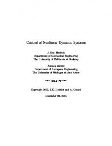
Ti max(zi)
x&1 = x1 + x 2 ,
T
x& 2 = x 22 + x3 x& 3 = x1 (1 +
x32 )
(4) +u
Fig. 1 Typical response of a state variable
If e.g. u is set equal to u18 67 u = x1 x32 +
a1 x1 + a 2 x 2 + a 3 x 3 + b1 x12 + b2 x 22 + .... 1444444424444444 3
This way, the following performance index Ji referring to the variable zi, to the desired states zD and to the initial conditions z0 is defined: (5)
u2
then eq. (4) can be written: x&1 = x1 + x 2 , x& 2 = x 22 + x3
(6)
x& 3 = (1 + a1 ) x1 + a 2 x 2 + a 3 x3 + b1 x12 + b2 x 22 + ...
The nonlinear system (6) is the result of intuition or previous analyses (term u1) and of a systematic {polynomial type) synthesis procedure (term u2). The performance of (6) depends now on the choice of the polynomial coefficients ai, bi etc.
3 Problem Solution The solution of the synthesis problem depends significantly on the appropriate definition of the performance index J. The structure of the proposed performance index is explained using Fig. 1. From the typical time response of a state variable, e.g. of zi, one may deduct the following characteristics: The maximum overshooting Sij of the variable zi(t) with respect to a given desired state zD and initial conditions z(t=0)= z0 Si
(8)
max( z i ) / z D
(7)
The end-position Zi(T) and -velocity Vi(T) of the variable zi(t) at prescribed simulation time T
Ji =
1
S i+ +
2
Z i+ (T ) +
3
Vi + (T ) + t
(9)
In (9) the upper indices “+” denote that the functions are defined only for positive arguments (otherwise =0) while = weighting factors If within a given observation period T S i+ , Z i+ (T ) and Vi + (T ) become zero, the computation is stopped immediately and the performance index Ji is then equal to t=Ti. Ji represents in this case the response time of the system with respect to the variable zi, the desired states zD and the initial conditions z0. Thus Jj is equal to:
Ji =
Ti if S i+ = Z i+ (T ) = Vi + = 0 otherwise = J i [z 0 , z D , T ]
(10)
The total performance index J of the dynamic system within the observation time period T is then equal to the sum:
J [z 0 , z D , T ] =
J i [z 0 , z D , T ]
(11)
i
The most important parameter is the observation time T. In this context it has to be noticed, that if T is initially chosen small and is gradually increased, this helps avoiding local minima from (11). This is a computing rule that has been derived from numerous numerical experiments. If this and other rules are applied, then deterministic parameter optimization methods, e.g.
the Nelder-Mead algorithm (FMINSEARCH of MATLAB), can be successfully used. Else, evolution strategy methods have to be applied to localize the global optimum.
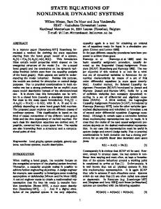
4 Test Problem In this section, the proposed methodology is applied to a test problem, not yet included in [8][22]. The dynamic system is shown in Fig. 2. Mass m2 is connected to m1 through a spring k1 and a modulated damper c1. m2 is excited through the spring k2 and the disturbance z0(t). The equations of motion of the dynamic system and of the actuator (time constant Tact and limit flim) are the following:
f
5 Numerical Results We demonstrate the proposed method, starting with bi=0, z1D= z2D=10 and T=10 sec. The initial avalues are chosen arbitrary, e.g.
a = [a1 ...a4 ] = [100 0 0 0]
(15)
Using the ‘fminsearch’ (Melder Nead) subroutine of MATLAB, the results shown in Fig. 3 are obtained.
c1
k1
Fig. 2 Dynamic system
m1 &z&1 + c1 ( z&1 z& 2 ) f + k1 ( z1 z 2 ) = 0 m2 &z&2 c1 ( z&1 z& 2 ) + f k1 ( z1 z 2 ) Tact
are also added. flim is supposed to be critical, therefore flim