Synthesizing Switching Logic for Safety and DwellTime Requirements
Susmit Kumar Jha Sumit Gulwani Sanjit A. Seshia Ashish Tiwari
Electrical Engineering and Computer Sciences University of California at Berkeley Technical Report No. UCB/EECS-2010-28 http://www.eecs.berkeley.edu/Pubs/TechRpts/2010/EECS-2010-28.html
March 10, 2010
Copyright © 2010, by the author(s). All rights reserved. Permission to make digital or hard copies of all or part of this work for personal or classroom use is granted without fee provided that copies are not made or distributed for profit or commercial advantage and that copies bear this notice and the full citation on the first page. To copy otherwise, to republish, to post on servers or to redistribute to lists, requires prior specific permission. Acknowledgement The UC Berkeley authors were supported in part by NSF grants CNS0644436 and CNS-0627734, and by an Alfred P. Sloan Research Fellowship. The fourth author was supported in part by NSF grants CNS0720721 and CSR-0917398 and NASA grant NNX08AB95A.
Synthesizing Switching Logic for Safety and Dwell-Time Requirements Susmit Jha
Sumit Gulwani
Sanjit A. Seshia
Ashish Tiwari
UC Berkeley
[email protected]
Microsoft Research
[email protected]
UC Berkeley
[email protected]
SRI International
[email protected]
Abstract—Cyber-physical systems (CPS) can be usefully modeled as hybrid automata combining the physical dynamics within modes with discrete switching behavior between modes. CPS designs must satisfy safety and performance requirements. While the dynamics within each mode is usually defined by the physical plant, the tricky design problem often involves getting the switching logic right. In this paper, we present a new approach to assist designers by synthesizing the switching logic, given a partial system model, using a combination of fixpoint computation, numerical simulation, and machine learning. Our technique begins with an overapproximation of the guards on transitions between modes. In successive iterations, the over-approximations are refined by eliminating points that will cause the system to reach unsafe states, and such refinement is performed using numerical simulation and machine learning. In addition to safety requirements, we synthesize models to satisfy dwell-time constraints, which impose upper and/or lower bounds on the amount of time spent within a mode. We demonstrate using case studies that our technique quickly generates intuitive system models and that dwell-time constraints can help to tune the performance of a design.
I. I NTRODUCTION As cyber-physical systems (CPS) are increasingly deployed in transportation, health-care, and other societalscale applications, there is a pressing need for automated tool support to ensure dependability while enabling designers to meet shortening time-to-market constraints. Modelbased design tools enable designers to work at a high level of abstraction, but there is still a need to assist the designer in creating correct and efficient systems. A holy grail for the design of cyber-physical systems is to automatically synthesize models from safety and performance specifications. In its most general form, automated synthesis is very difficult to achieve, in part because synthesis often involves human insight and intuition, and in part because of system complexity – the tight integration of complex continuous dynamics with discrete switching behavior can be tricky to get correct. Nevertheless, in some contexts, it may be possible for automated tools to complete partial designs generated by a human designer, thus enabling the designer to efficiently explore the space of design choices whilst ensuring that the synthesized system remains safe. In this paper, we consider a special class of synthesis problems, namely synthesis of mode switching logic for
multi-modal dynamical systems (MDS). An MDS is a physical system (plant) that can operate in different modes. The dynamics of the plant in each mode is known. However, to achieve safe and efficient operation, it is often necessary to switch between the different operating modes. Designing correct switching logic can be tricky and tedious. We consider the problem of automatically synthesizing switching logic, given the intra-mode dynamics, so as to preserve safety in MDS. The human designer can guide the synthesis process by providing initial approximations of the switching guards and a library of expressions (components) using which the guards can be synthesized. Our synthesis approach performs reasoning within each mode and reasoning across modes in two different ways. Within each mode, reasoning is based entirely on using numerical simulations. While this can lead to potential unsoundness, it allows us to handle complex and nonlinear dynamics that are difficult to reason about in any other way. Across modes, reasoning is performed using fixpoint computation techniques. Similar to abstract interpretation, computation of the fixpoint is performed over an “abstract domain,” which is specified by the user in the form of a component library for the switching guards. Each step of the fixpoint computation involves the use of machine learning to learn improved approximations of the switching guards based on the results of numerical simulations. The key contribution of our paper is a new approach for synthesizing safe switching logic based on integrating numerical simulation, machine learning, and fixpoint iterations. In addition to safety, our approach also extends to handling dwell-time requirements, which impose upper and/or lower bounds on the amount of time spent within a mode. While numerical simulations have been used to perform formal verification (e.g., [7], [5], [4]), to our knowledge our approach is the first to use simulations to perform synthesis with safety guarantees. We demonstrate using case studies (Sec. III and VI) that our technique generates intuitive system models and that dwell-time constraints can help to tune the performance of a design. II. P ROBLEM D EFINITION In this section, we describe the problem of synthesizing switching logic for a multi-modal continuous dynamical
A safety property is a set φS ⊆ Rn of states. We will overload φS to also denote the predicate φS (X). A state x is said to be safe if and only if x ∈ φS (or equivalently, if φS (x) is true). A hybrid system HS is safe with respect to φS if and only if all the reachable states in HS are safe. Coming up with the correct guards for the mode switches such that all reachable states are safe is challenging and our proposed technique aims at automating this task. While controller synthesis has been widely studied, what differentiates our work is that we provide the designer an option to provide some initial partial design. Specifically, we assume that the designer can provide an over-approximations for the guards. In the extreme case, if transition from mode i to mode j is disallowed, then the designer can set gij = ∅, and if the designer knows nothing about the possibility of a transition from mode i to mode j, then she can set gij = Rn . The designer can specify partial information by picking an intermediate set as the initial guard. ′ If S := h(gij )i,j∈M i and S ′ := h(gij )i,j∈M i are two switching logics, then we use the notation S ′ ⊆ S to denote ′ that gij ⊆ gij for all i, j ∈ M . We provide two variants of the problem definition. Definition 3 (Switching logic synthesis problem v1): Given a multi-modal continuous dynamical system (MDS), a switching logic S, and the safety specification φS , the switching logic synthesis problem seeks to synthesize a new switching logic S ′ such that (1) S ′ ⊆ S and (2) the hybrid system HS := (MDS, S ′ ) is safe with respect to φS . Consider the case when the designer provides no information and sets all guards to Rn . In this case, it is trivial to synthesize a safe hybrid system by just setting all switching guards to be φS . The reader can check that this is a solution for the switching logic synthesis problem defined above. This solution is, however, undesirable since the resulting hybrid system has only zeno behaviors, i.e., an infinite number of transitions can be made in finite time (as we are assuming that a transition is taken as soon as it is enabled). The second problem definition below gives the designer a way to explicitly rule out solutions that have zeno behavious. Specifically, the user can specify (both lower and upper) bounds on the amount of time every trajectory should spend in a mode. Definition 4 (Switching logic synthesis problem v2): Given a multi-modal continuous dynamical system (MDS), a switching logic S, a sequence hte1 , . . . , tek i of non-negative minimum-dwell time requirements, a sequence htx1 , . . . , txk i of non-negative maximum-dwell time requirements, and a safety specification φS , the switching logic synthesis problem seeks to synthesize a new switching logic S ′ such that (1) S ′ ⊆ S, (2) the hybrid system HS := (MDS, S ′ ) is safe with respect
system. We present two versions of the problem. In the first version, we ask for a switching logic that only preserves safety. In the second version, we also require that the synthesized system satisfy some dwell-time requirements in each mode. We begin with some definitions. A continuous dynamical system (CDS) is a tuple hX, f i where X is a finite set of |X| = n real-valued variables that define the state space Rn of the continuous dynamical system, and f : Rn 7→ Rn is a vector field that specifies the continuous dynamics as dx dt = f (x). The vector field f is assumed to be locally Lipschitz at all points, which guarantees the existence and uniqueness of solutions to the ordinary differential equations. Often, a system has multiple modes and in each mode, its dynamics is different. Such a multi-modal system behaves as a different continuous dynamical system in each mode. Definition 1 (Multi-modal CDS (MDS)): An MDS is a tuple hX, I, f1 , f2 , . . . , fk i where • hX, fi i is a continuous dynamical system (representing the i-th mode) • I ⊆ Rn is the set of initial states We will use M = {1, 2, . . . , k} as the set of indices of the modes. A trajectory for MDS is a continuous function τ (t) : [0, ∞) 7→ Rn if there is an increasing sequence t0 := 0 < t1 < t2 . . . such that • τ (0) ∈ I, • for each interval [ti , ti+1 ), there is some mode j ∈ M such that dτ dt (t) = fj (τ (t)) for all ti ≤ t < ti+1 , and • j = 1 when ti = 0 (that is, we start in Mode 1.). A multi-modal system can nondeterministically switch between its modes. The goal is to control the switching between different modes to achieve safe operation. Definition 2 (Switching logic (S)): A switching logic S for an MDS hX, I, (fi )i∈M i is a tuple h(gij )i6=j;i,j∈M i, containing guards gij ⊆ Rn . A multi-modal system MDS can be combined with a switching logic S to create a hybrid system HS := (MDS, S) in the following natural way: the hybrid system HS has k modes with dynamics given by dX dt = fi in mode i, and with gij being the guard on the discrete transition from mode i to mode j. The initial states of HS are I in Mode 1, where I is the set of initial states of the MDS. The discrete transitions in HS have identity reset maps, that is, the continuous variables do not change values during discrete jumps. The state invariant Inv i for a mode i ∈ I is the (topological) closure of the complement of the union of all guards on outgoing transitions; in other S words Inv i := Closure(Rn − j∈I gij ). Note that we are assuming here that a discrete transition is taken as soon as it is enabled.1 This completes the definition of the hybrid system. The semantics of hybrid systems that defines the set of reachable states of hybrid systems is standard [1]. 1 Assume that the mode dynamics are not tangential to the state invariant at any point.
2
HEATING (H)
gF H
OFF (F)
to φS , and (3) whenever any trajectory of HS enters mode i, it stays in mode i for atleast tei and atmost txi time units. The designer can now force the synthesis of only nonzeno systems by setting tei to a strict positive number for selected modes. Note that if the designer sets tei to zero and txi to ∞ for all modes, then the second problem is the same as the first problem.
x˙ = −0.002(x − 16) T˙ = 0
x˙ = −0.002(x − T ) T˙ = 0.1
gCF
gHN
x˙ = −0.002(x − T ) T˙ = −0.1
x˙ = −0.002(x − T ) T˙ = 0 gNC
ON (N)
COOLING (C)
Notation Fig. 1.
Our paper makes use of the formal definitions of temporal formulas and the evaluation of a temporal formula in a given dynamical system as given below. Consider the weak until W and the strong until U temporal logic operators. Recall that we do not distinguish between a set of states and a predicate on states. A state formula is a predicate on states or a Boolean combination of predicates. If φ, φ′ are sets of states, then φWφ′ and φUφ′ are temporal formulas. A state formula is evaluated over a state. The formula φ evaluates to true on a state x if x ∈ φ. A temporal formula is evaluated over a given trajectory τ . The formula φUφ′ evaluates to true on trajectory τ if ∃t0 : τ (t0 ) ∈ φ′ ∧ (∀0 ≤ t < t0 : τ (t) ∈ φ)
20◦ C, that is, φS is 18 ≤ x ≤ 20. (We omit the units in the sequel, for brevity.) In the OFF mode, the temperature falls at a rate proportional to the difference between the room temperature x and the temperature outside the room which is assumed to be constant at 16. In the HEATING mode, the heater heats up from 20 to 22 and in the COOLING mode, the heater cools down from 22 to 20. In the ON mode, the heater is at a constant temperature of 22. In the HEATING, ON and COOLING mode, the temperature of the room changes in proportion to the difference between the room temperature and the heater temperature. We need to synthesize the four guards: gF H , gHN , gN C and gCF . The guards must respect the safety property on the room temperature x as well as the specification on the heater temperature T in HEATING and COOLING mode. So, from the given specifications, we know that
(1)
Informally, the temporal formula φUφ′ is true if φ′ becomes true eventually and until it becomes true, φ is true. The weak until operator, W, is a weaker notion and does not require that φ′ necessarily becomes true. If φ, φ′ are sets of states, then the temporal formula φWφ′ evaluates to true over a given trajectory τ if
gF H gHN gNC gCF
(∃t0 : τ (t0 ) ∈ φ′ ∧ (∀0 ≤ t < t0 : τ (t) ∈ φ)) ∨ (∀t ≥ 0 : τ (t) ∈ φ)
(2)
|=
⊆ 18 ≤ x ≤ 20 ∧ T ⊆ 18 ≤ x ≤ 20 ∧ T ⊆ 18 ≤ x ≤ 20 ∧ T ⊆ 18 ≤ x ≤ 20 ∧ T
= 20 = 22 = 22 = 20
(3)
In order that the MDS remains safe, we need to ensure that all states reachable within each mode are safe. Consider the OFF mode. We need to ensure that all traces starting from some point in the initial condition I or gCF do not reach an unsafe state before reaching some state in gF H . Reaching some state in gF H enables a transition out of the OFF mode. In other words, the first two temporal properties in Equation 4 must be satisfied by all traces in the OFF mode. Similarly, for HEATING mode, all traces starting from some state in x ∈ gF H must not reach an unsafe state before reaching an exit state in gHN , as indicated by the third property below. For the other two modes, similar temporal properties on the traces need to be enforced. Overall, the following temporal assertions can be written for the four guards.
For uniformity, a state formula can be evaluated on a trajectory as follows: a state formula φ evaluates to true on a trajectory τ if τ (0) ∈ φ. We can combine state and temporal formulas using Boolean connectives and evaluate them over trajectories using the natural interpretation of the Boolean connectives. If Φ is a state or temporal formula, then we write Mode i , I
Thermostat
Φ
to denote that the formula Φ evaluates to true on all trajectories of the CDS in mode i that start from a state in I.
F, I F, gCF H, gF H N, gHN C, gNC
III. OVERVIEW In this section, we present an overview of our approach using a thermostat controller [9] as an example. The 4mode thermostat controller is presented in Figure 1. The room temperature is represented by x and the temperature of the heater is represented by T . The initial condition I is given by T = 20◦ C and x = 19◦ C. The safety requirement φS is that the room temperature lies between 18◦ C and
|= |= |= |= |=
φS φS φS φS φS
W W W W W
gF H gF H gHN gNC gCF
(4)
Switching Logic Synthesis Problem v1: We can synthesize a safe switching logic by computing the fixpoint of the above 5 assertions in Equation 4. We initialize using the equations 3
in Equation 3 obtained from the safety and other user provided specifications which put an upper bound on the guards. We then perform a greatest fixpoint computation: in each iteration, we remove states from the guards which would lead to some unsafe state in a mode. Fixpoint computation leads to the following guards which ensure that all states reachable are safe. We compute only till the second place of decimal. gF H gHN gNC gCF
: 18.00 : 18.00 : 18.00 : 18.00
≤ x ≤ 19.90 ∧ T ≤ x ≤ 19.95 ∧ T ≤ x ≤ 19.95 ∧ T ≤ x ≤ 20.00 ∧ T
tions in (4) and (5) are as follows. gF H gHN gNC gCF
18.00 18.00 18.35 18.45
≤ x ≤ 19.90 ∧ T ≤ x ≤ 19.95 ∧ T ≤ x ≤ 19.95 ∧ T ≤ x ≤ 20.00 ∧ T
= 20 ∧ t ≥ 100 = 22 = 22 = 20
Since t was a timer variable we had introduced, we next eliminate it from gF H . We do so by removing states from gF H which are reachable from any state in gCF in less than 100 seconds. These set of states are 18.01 < x ≤ 20 ∧ T = 20. Hence, the final guards that respect the safety property as well as enforce a minimum dwell-time of 100 seconds in OFF mode are as follows.
= 20 = 22 = 22 = 20
The behavior of the synthesized thermostat for the first 1000 seconds from the initial state is shown in Figure 2. The room temperature gradually rises from its initial value of 19 and then stays between 19.90 and 20.
gF H gHN gNC gCF
23 Temperature(celsius)
: : : :
: 18.00 : 18.00 : 18.00 : 18.00
≤ x ≤ 18.01 ∧ T ≤ x ≤ 19.95 ∧ T ≤ x ≤ 19.95 ∧ T ≤ x ≤ 20.00 ∧ T
= 20 = 22 = 22 = 20
The behavior of the synthesized thermostat for the first 1000 seconds from the initial state is shown in Figure 3. We observe that the number of switches has gone down from 21 to 5 and the room temperature now stays between 18.01 and 18.45.
22 21 20 Room temperature 19
Heater temperature 23 200
400
600
800
1000
Temperature(celsius)
18 0
Time(sec)
Fig. 2.
Behavior of Synthesized Thermostat
Switching Logic Synthesis Problem v2: Though the system synthesized above satisfies the safety specification, it has the undesirable behavior of switching frequently. It keeps the room temperature in the narrow interval of 19.90 ≤ x ≤ 20, even though the safety condition only required it to be in 18 ≤ x ≤ 20. Ideally, designers are interested not only in safe systems but in systems with good performance. The dwell time specification provides a mechanism to the designer to guide our synthesis technique to solutions with good performance. Minimum dwell-time of 100 seconds in OFF mode (case A): We add an extra constraint in the specification of our synthesis problem that the system must spend atleast 100 seconds in the OFF mode. This would lead to less frequent switching as well as minimize energy consumption since heater remains off in the OFF mode. Let us add a timer variable t with dynamics t˙ = 1 in every mode. Assume that t is reset to 0 during every discrete transition. To enforce the minimum dwell-time, the following constraint must also be satisfied in addition to the fixpoint constraints in Equation 4. F, I F, gCF
|= |=
φS W (gF H ∧ t ≥ 100) φS W (gF H ∧ t ≥ 100)
22 21 20 Room temperature Heater temperature
19 18 0
200
400
600
800
1000
Time(sec)
Fig. 3. Behavior of Synthesized Thermostat with Dwell Time Specification: Minimum dwell time of 100s in OFF mode.
Minimum dwell-time of 300 seconds in both OFF and ON mode (case B): We observe that the design synthesized with minimum dwell-time of 100 seconds in OFF mode has relatively less switching but still, we would like to reduce its switching frequency. Also, the room temperature can safely lie between 18 and 20 but in the above synthesized system, it is restricted to a narrow interval of 18.01 and 18.45. So, we increase the minimum dwell-time in OFF mode to 300 seconds. We also enforce a minimum dwelltime of 300 seconds in ON mode to ensure room heats up to a higher temperature within the safe interval. We now get the following fixpoint equations. F, I F, gCF H, gF H N, gHN C, gNC
(5)
The guards obtained by computing the fixpoint of equa4
|= |= |= |= |=
φS φS φS φS φS
W W W W W
gF H ∧ (t ≥ 300) gF H ∧ (t ≥ 300) gHN gNC ∧ (t ≥ 300) gCF
S WITCH S YN 1(MDS, φS , S):
Fixpoint computation yields the following guards. gF H gHN gNC gCF
: : : :
18.00 18.00 19.60 19.65
≤ x ≤ 18.14 ∧ T ≤ x ≤ 18.26 ∧ T ≤ x ≤ 19.95 ∧ T ≤ x ≤ 20.00 ∧ T
1
= 20 ∧ t ≥ 300 = 22 = 22 ∧ t ≥ 300 = 20
2 3 4 5
We restrict gN C and gF H in the same way as (Case A) by computing the set of states reachable from gHN and gCF in less than 300 seconds respectively. The final synthesized guards are as follows. gF H gHN gNC gCF
: : : :
18.00 18.00 19.94 19.65
≤ x ≤ 18.01 ∧ T ≤ x ≤ 18.26 ∧ T ≤ x ≤ 19.95 ∧ T ≤ x ≤ 20.00 ∧ T
6 7 8 9
= 20 = 22 = 22 = 20
10 11 12 13 14
The behavior of the synthesized thermostat for the first 1000 seconds from the initial state is shown in Figure 4. We observe that the number of switches has gone down to 1 and the room temperature is still within the safe interval of 18 and 20. This example shows how our synthesis approach
15 16
Fig. 5.
Temperature(celsius)
Room temperature Heater temperature
21 20 19 18 0
200
400
600
800
1000
Time(sec)
Fig. 4. Behavior of Synthesized Thermostat with Dwell Time Specification: Minimum dwell time of 300s in OFF and ON modes.
can be used to synthesize not only safe systems but also systems with desired performance. Dwell-time properties can be used by the user to explore designs with better performance. IV. F IXPOINT A LGORITHM We are now ready to describe the procedure for solving the switching logic synthesis problem in Definition 3. Assume that we are given an MDS MDS, a safety property φS , and an over-approximation of the guards S. MDS := hX, I, f1 , . . . , fk i, φS ⊆ Rn , S := h(gij )i,j∈M i We wish to solve the problem in Def. 3 for these inputs. ′ Let us say we find guards gij ’s such that they have the following property: for every mode i, if a trajectory enters mode i (via any of the incoming transitions with guard ′ gji ), then it remains safe until one of the exit guards gik becomes true. This property can be written formally using the weak until operator. _ ′ Mode 1 , I |= φS W( g1k ) k∈M
_
′ Mode i , gji j∈M
|=
φS W(
_
Procedure for solving the switching logic synthesis problem v1.
If the guards in the switching logic S ′ satisfy the collection of assertions in Equation 6, then the resulting hybrid system is safe. The converse is also true. Lemma 1: Given an MDS := hX, I, f1 , . . . , fk i, and a ′ safety property φS , if S ′ = h(gij )i,j∈M i is a switching logic that satisfies all assertions in Equation 6, then the hybrid system HS := (MDS, S ′ ) is safe with respect to φS . Conversely, if there exists a switching logic S ′ such that the hybrid system HS := (MDS, S ′ ) is safe with respect to φS , then there is a switching logic S ′′ ⊆ S ′ that satisfies the assertions in Equation 6. Proof: The first part follows directly from the definition of the semantics of the temporal operators and our assumption that discrete transitions are taken as soon as they are enabled. ′′ For the converse part, the desired S ′′ := h(gij )i,j∈M i is obtained by intersecting the set Reach of reachable states ′ ′′ ∩ Reach. The reader can := gij of HS with S ′ ; that is, gij verify that S ′′ will satisfy the assertions in Equation 6. At a semantic level, we can solve the problem in Definition 3 by computing the fixpoint of the assertions in Equation 6. This procedure is presented in Figure 5. The fixpoint iterations start by picking the most liberal guards possible (which is the intersection of the safety property and the user-specified bounds). In each successive step, the guards are made smaller by removing certain “bad” states. ′ Specifically, we remove from gji any state that reaches an unsafe state following the dynamics of Mode i, before it reaches any exit guard. Thus, in each iteration, we reason locally about only one mode at a time. We stop when we reach a fixpoint. We state the soundness and completenss of the fixpoint algorithm for solving the switching logic synthesis problem. Lemma 2: If Procedure S WITCH S YN 1 terminates with ′ “synthesis successful” and gij are the discovered guards,
23 22
// Input MDS := hX, I, f1 , . . . , fk i, // Input φS ⊆ Rn , // Input S := h(gij )i,j∈M i, // Output synthesis successful/failed ′ for all i, j ∈ M do gij := gij ∩ φS repeat { for all i ∈ M do { W ′ )U¬φS } bad := {x | Mode i , {x} |= ¬( k gik ′ ′ for all j ∈ M do gji := gji − bad if (i == 1 and I ∩ bad 6= ∅) return "synthesis failed" } ′ } until (gij ’s do not change) if (I ⇒ φS ) return "synthesis successful" else return "synthesis failed"
′ gik ) for i = 1..k (6)
k∈M
5
′ ′ ′ Suppose S ′′ ⊆ SN . Suppose we go from SN to SN +1 ′ by deleting the set bad from gji . We need to show that ′ ′ ′ ′′ S ′′ ⊆ SN := +1 . Let SN := h(gN ij )i,j∈M i and let S ′′ h(gij )i,j∈M i.
then these guards satisfy all the assertions in Equation 6. Proof: If Procedure S WITCH S YN 1 returns “synthesis successful”, then the condition in Step 10 must be false, that is, I ∩ bad = ∅. So, from the definition of bad W , ′there does )U¬φS . not exist x ∈ I such that Mode 1 , {x} |= ¬( k g1k For all states x ∈ I, _ ′ Mode 1 , {x} |= φS W( g1k )
x ∈ bad _ ′ )U¬φS ⇒ Mode i , {x} |= ¬( gNik k
_
′′ ′′ ′ gik )U¬φS , ∵ gik ⊆ gNik
k∈M
⇒
Mode i , {x} |= ¬(
_
⇒
Mode i , {x} |= ¬(φS W
⇒
Mode i , {x} 6|= φS W
⇒
′′ x 6∈ gji , ∵ S ′′ satisfies Equation 6 x 6∈ I if i == 1, ∵ S ′′ satisfies Equation 6
k
that is, Mode 1 , I |= φS W(
′ g1k )
Also, if Procedure S WITCH S YN 1 returns “synthesis successful”, the termination condition for repeat loop at ′ ′ Step 13 must be true. So, for all i ∈ M the gji = gji − bad ′ for all j ∈ M , that is gji ∩ bad is empty. So, for all ′ for any j such i ∈ M , there does notWexist any x ∈ gji ′ that Mode i , {x} |=W ¬( k gik )U¬φS . So, for all i ∈ M , ′ for any state x in j∈M gji , _ ′ Mode i , {x} |= φS W( gik ) _
′ gji |= φS W(
j∈M
Thus, the discovered guards in Equation 6.
_
′′ gik
′ This shows that S ′′ ⊆ SN +1 and Procedure S WITCH S YN 1 cannot return at Line 11. Since HS is assumed to be safe, I ⇒ φS and hence Procedure S WITCH S YN 1 cannot return at Line 16. Hence, Procedure S WITCH S YN 1 can only return “synthesis successful” contradicting our assumption.
A. Switching Logic Synthesis V2
′ gik )
We now consider the switching logic synthesis problem in Definition 4. Recall that apart from the bounds on the guards, the user can provide minimum and maximum dwell time requirements for each mode. The goal is to synthesize a switching logic where the guards satisfy the specified bounds and the trajectories of the resulting hybrid system satisfy the minimum and maximum dwell time requirements. Procedure S WITCH S YN 2 for solving the problem in Definition 4 is outlined in Figure 6. Procedure S WITCH S YN 2 runs in three phases. In the first step, the new problem is transformed to the old problem. In the second step, Procedure S WITCH S YN 1 is used to solve the generated problem. In the third step, the result is transformed back to get a result of the given problem. Suppose that we are given
k∈M ′ gij
_ k
k∈M
Mode i ,
′′ gik )
k
k∈M
that is,
_
satisfy all the assertions
Theorem 1 (Soundness of Procedure S WITCH S YN 1): If Procedure S WITCH S YN 1 terminates with “synthesis ′ successful” and gij are the discovered guards, then the ′ hybrid system HS := (MDS, h(gij )i,j∈M i) is safe for φS . Proof: Using Lemma 1 and Lemma 2, we conclude that the hybrid system HS := (MDS, S ′ ) is safe with respect to φS . Even when it terminates with success, note that the Procedure S WITCH S YN 1 does not guarantee that the synthesized hybrid system HS has nonzeno behaviors. In a post-processing step, one can perform sufficient checks to guarantee the absence of zeno behaviors. We can also show that our procedure is complete. Theorem 2 (Completeness of Procedure S WITCH S YN 1): If Procedure S WITCH S YN 1 terminates with “synthesis failed”, then there is no S ′ ⊆ S such that the hybrid system HS := (MDS, S ′ ) is safe. Proof: Assume that the claim is false and there is a switching logic S ′ ⊆ S such that HS := (MDS, S ′ ) is safe. By Lemma 1, there is a switching logic S ′′ := Reach ∩ S ′ that satisfies Equation 6. Recall that Reach is the set of reachable states of HS. Let Si′ , i = 0, 1, . . ., be the intermediate switching logics computed by Procedure S WITCH S YN 1. Clearly, S0′ ⊇ S1′ ⊇ S2′ ⊇ · · · and S0′ := S ∩ φS . Since Reach ⊆ φS by assumption, we can easily verify that S ′′ ⊆ S0′ . We will inductively show that S ′′ ⊆ Si′ for all i.
MDS := hX, I, f1 , . . . , fk i, φS ⊆ Rn , S := h(gij )i,j∈M i, Te := {te1 , . . . , tek }, Tx := {tx1 , . . . , txk } In the first step, the problem in Definition 4 is reduced to the previous problem. This reduction is achieved by introducing a new state variable t such that (1) the dynamics of t is given by t˙ = 1 in each mode (2) the variable t is reset to 0 in each discrete transition These two steps are performed by the function Add timer t. Now, the dwell time requirements can be specified as bounds on the variable t. Specifically, the over-approximation S of the guards can be updated as follows: gij 6
:= gij ∧ (tei ≤ t ≤ txi )
S WITCH S YN 2(MDS, φS , S, Te, Tx):
In the second step, a call to Procedure S WITCH S YN 1 is made, but with the updated S. Recall that Procedure S WITCH S YN 1 essentially performs an iterative fixpoint computation to solve Equation 6. Equation 6 assumes that discrete transitions do not reset any continuous variables. Since we now have discrete transitions that reset t to 0, we need a slightly modified Procedure S WITCH S YN 1 that solves the modified equations below: _ ′ Mode 1 , R(I) |= φS W g1k
1 2 3 4 5 6 7 8 9
k∈M
Mode i ,
_ ′ R(gji ) |= j∈M
φS W
10
_ ′ gik for i = 1..k (7)
11 12
k∈M
13
where R(S) is the set of states obtained by resetting the tcomponent of every state in the set S to 0. If φ is a formula denoting the set S, then R(φ) is ∃s(φ[s/t] ∧ t = 0) (the notation φ[s/t] means replace t by s in φ). Informally, R(φ) can be computed by first removing facts about t from φ and then adding the new fact t = 0 to it. The guards synthesized by Procedure S WITCH S YN 1 will use the new state variable t. However t was not part of our original problem specification. In the third step, the variable t is eliminated from the guards synthesized by ′ )i,j∈M i is the Procedure S WITCH S YN 1. Suppose S ′ := h(gij switching logic synthesized by Procedure S WITCH S YN 1. We first project out the t-component from S ′ to get our first guess for the desired S. Then, for every mode i, and for ′ ′ , each entry guard, say gji , and for each exit guard gik ′ we compute pairs of states (x, x ) such that x ∈ gji , x′ ∈ gik , there is a trajectory in mode i that starts from state hx, t = 0i and reaches hx′ , t′ i in time t′ , and hx′ , t′ i ′ is not in gik . A behavior where mode i in entered in state x and exited in x′ was disallowed in S ′ , but it is allowed in S (since S ignores t). Hence, we need to either remove x from gji , or remove x′ from gik . Procedure S WITCH S YN 2 procedure non-deterministically makes this choice. Removal of states from the guards can potentially cause the modified switching logic to become unsafe. Hence, in the final step, we need to verify that the updated guards still satisfy Equation 6. This is performed by the function Verify. The function Verify can be implemented by calling Procedure S WITCH S YN 1 and checking its return value. We can now state the soundness and completenss of Procedure S WITCH S YN 2 for solving the switching logic synthesis problem in Def. 4. Theorem 3 (Soundness of Procedure S WITCH S YN 2): If Procedure S WITCH S YN 2 terminates with “synthesis ′ successful” and gij are the discovered guards, then the ′ )i,j∈M i) is safe for φS hybrid system HS := (MDS, h(gij and it satisfies the dwell time requirements specified by Te and Tx. Proof: The final Verify check guarantees that HS is safe with respect to φS . The over-approximation defined in Step 6 of Procedure S WITCH S YN 2 ensures that the switching
14 15 16 17 18 19 20 21 22 23
// Input MDS, φS , S: As in Figure 5 // Input Te := hte1 , . . . , tek i // Input Tx := htx1 , . . . , txk i // Output synth. successful/failed MDSe := Add_timer_t(MDS) S e := h(gij ∧ (tei ≤ t ≤ txi ))i,j∈M i // Call S WITCH S YN 1 with the updated S res := S WITCH S YN 1(MDSe , φS , S e ) if res == "synthesis failed" return "synthesis failed" else let S ′ be the synthesized guards // post processing step for all i, j ∈ M do ′ gij := {x | hx, ti ∈ gij } for all i, j, k ∈ M do { ′ bad := {hx, x′ i | x ∈ gji ∧ x′ ∈ gik ∧ hx′ , t′ i 6∈ gik ′ ′ ∧ Mi , {hx, t = 0i} |= trueU{hx , t i}} Guess B1 , B2 s.t. B1 × B2 ⊇ bad gji := gji − B1 ; gik := gik − B2 } if (Verify(MDS, φS , h(gij )i,j∈M i)) return "synthesis successful" else return "synthesis failed"
Fig. 6.
Procedure for solving the switching logic synthesis problem v2.
logic S ′ synthesized by Procedure S WITCH S YN 1 on Line 8 satisfies the dwell time requirements. From Theorem 1, the guards also satisfy the following. _ _ ′ ′ Mi , gji |= φS W( gik ) j∈M
k∈M
From Step 16, it follows that _ _ ′ ′ Mi , gji |= (¬ gik )W(t ≥ tei ) j∈M
k∈M
′ gij ’s
So, the guards synthesized by Procedure S WITCH S YN 2 satisfy the following assertions _ _ ′ ′ Mi , gji |= (φS ∧ ¬ gik )W(t ≥ tei ) j∈M
k∈M
for all i ∈ M
(8)
So, the synthesized guards define a switching logic that satisfies the requirements in Problem Definition 4. We can also state and prove completeness of Procedure S WITCH S YN 2. Theorem 4 (Completeness of Procedure S WITCH S YN 2): If, for every possible guess on Line 18, the Procedure S WITCH S YN 2 terminates with “synthesis failed”, then there is no S ′ ⊆ S such that the hybrid system HS := (MDS, S ′ ) is safe and it satisfies the dwell time requirements. Proof: The completeness of the algorithm follows from the non-deterministic guesses in Step 18. The Procedure S WITCH S YN 2 first transforms the problem to an 7
the following properties: if bad ∈ C, then out L = bad ; otherwise, out L ⊇ bad . For simplicity, we describe below how L can be implemented when bad is an interval constraint on a single variable. It is possible to extend this method to conjunctions of interval constraints on multiple variables. An exploration of extensions to more complicated sets is left to future work.
extended MDS and uses Procedure S WITCH S YN 1 to compute the guards (Step 8). By Theorem 2, we know that Procedure S WITCH S YN 1 is complete. So, if there is a switching logic that produces a MDS which is safe and satisfies dwell-time properties, then guards computed in Step 8 will contain this switching logic. Hence, the only place where completeness might be compromised is in the post-processing step. However, we make non-deterministic guesses for removing states from the guards computed by Procedure S WITCH S YN 1 and hence, if a solution exists, we can always guess the correct sets to be substracted from the computed guards in Step 18 such that we obtain the desired solution. This gives us the desired completeness result. Procedure S WITCH S YN 2 is nondeterministic and involves making the correct guesses in the postprocessing stage. We can get a deterministic version of the procedure by making arbitrary guesses at each point. This deterministic version will be sound: whenever the procedure outputs “synthesis successful”, the synthesis problem in Definition 4 indeed has a positive answer. However, it will not be complete: even when there is a positive answer for the synthesis problem, the deterministic variant can fail to find the appropriate guards because it can make the wrong choices. Some form of backtracking appears to be required. In practice, our implementation’s heuristically-guided choices have always obtained a positive answer. V. L EARNING G UARDS
FROM
B. Simulation Oracles We assume the availability of the following two kinds of simulation-based oracles: • Oracle SO A : This is an oracle that, given a state x, the dynamics of a mode Mode i , and state sets φ1 and φ2 , returns a Boolean answer indicating whether the following property holds: Mode i , {x} |= (φ1 Uφ2 ) Note that definition of SO A is motivated by the need to compute bad in Line 8 of Procedure S WITCH S YN 1. • Oracle SO B : This is an oracle that, given a state pair hx, x′ i, the dynamics of a mode Mode i , extended-state set ψ, and state sets φ1 and φ2 , returns a Boolean answer indicating whether the following property holds: x ∈ φ1 ∧ x′ ∈ φ2 ∧ hx′ , t′ i 6∈ ψ ∧ Mode i , {hx, 0i} |= (trueUhx′ , t′ i)
S IMULATIONS
The definition of SO B is motivated by the need to compute bad in Line 17 of Procedure S WITCH S YN 2. Implementing these oracles involves performing a simulation from state x according to the (deterministic) dynamics in Mode i , checking whether the condition on the RHS of the U operator has become true, and if not, checking that the LHS condition remains true. We assume the presence of a numerical simulator that can, for the mode dynamics of interest, select an appropriate discretization of time so as to check the above formulas with the U operator.
A key step in the implementation of Algorithms S WITCH S YN 1 and S WITCH S YN 2 is the computation of the bad state sets. In general, since the mode dynamics can be non-linear and quite complex, exactly computing the bad sets through analytical means is computationally infeasible. However, it is easier to perform numerical simulation of even complex, non-linear dynamics from individual points. In particular, in many cases, numerical simulation can be used to check whether a point x is a member of bad . Given such a membership check, our approach uses machine learning to compute an over-approximation of bad . While such overapproximation can result in a loss of completeness, it is guaranteed to generate safe switching logic.
C. Learning Interval Constraints We now describe how one can implement L for learning an interval constraint over a single variable x ∈ X. This form of constraint suffices for learning guards for all examples we consider in this paper. We give conditions under which the algorithm presented here satisfies the conditions required of L as stated above in Sec. V-A. An interval constraint is of the form x ∈ [li , ui ] where li , ui ∈ Q. This constraint can also be expressed using inequalities as li ≤ x ≤ ui . Thus, C is the set of all constraints of the form x ∈ [li , ui ] for any li , ui ∈ Q and for any x ∈ X. The initial overapproximation c and the set out L generated by L are both representable as an interval constraint. Algorithm LC begins by checking the end-points of c = [l, u] for membership in bad . If both l and u are in bad , it simply outputs out L = c. Otherwise, it selects the
A. Machine Learning Our procedure assumes the availability of a machine learning algorithm L that can learn any target set from a concept class C. L uses an oracle that can label points x as being in the target concept (i.e., x ∈ bad ) or not in it (i.e. x 6∈ bad ). L is parameterized by C, a point we sometimes make explicit by writing LC rather than L. Formally, given the following three inputs: (i) an overapproximation c ∈ C of the set bad ; (ii) a simulation oracle that can label a point x as x ∈ bad or x 6∈ bad ; and (iii) (optionally) a sample of examples P ⊆ bad (if they exist), LC must generate as output a set out L ∈ C with 8
minimum and maximum elements xmin and xmax in the set of examples P ∈ bad . (If P is not provided as input, L will randomly sample elements of out L until an example P ∈ bad is found). We assume that the interval [l, u] can be suitably discretized so that the extreme points of bad are members of this discretized set of points. Since guards are implemented using finite-precision software, this assumption is not restrictive. L then performs binary search in the ranges [l, xmin ] and [xmax , u] until it finds two examples xl ∈ [l, xmin ] and xu ∈ [xmax , u] such that xl , xu ∈ bad where xl is the smallest such point and xu is the largest. It then outputs out L = [xl , xu ]. It is easy to see that if bad ∈ C, then out L = bad . However, if bad 6∈ C, then bad must be a disjoint union of intervals. Under the condition that P contains one point from each interval in this union, we obtain out L ⊃ bad . Alternatively, suppose that the dynamics within each mode i is such that each state variable evolves monotonically with time – i.e., its value within that mode either increases with time or it decreases, but not both. In this case, bad cannot be a disjoint union of intervals, and so out L = bad . All examples discussed in this paper have this monotonicity property.
Iter.
lF H , uF H
lHN , uHN
lNC , uNC
lCF , uCF
0 1 2 3 4
18.00, 20.00 18.00, 19.95 18.00, 19.95 18.00, 19.90 18.00, 19.90
18.00, 20.00 18.00, 20.00 18.00, 19.95 18.00, 19.95 18.00, 19.95
18.00, 20.00 18.00, 19.95 18.00, 19.95 18.00, 19.95 18.00, 19.95
18.00, 20.00 18.00, 20.00 18.00, 20.00 18.00, 20.00 18.00, 20.00
TABLE I S TEPS OF F IXPOINT C OMPUTATION FOR T HERMOSTAT V 1
E. Examples We illustrate this with an example from our experiments. For the thermostat example in Figure 1, the room temperature x varies monotonically in the heating mode. We also start with an over-approximation for the guard from off to heating mode gF H that gF H ⊆ 18 ≤ x ≤ 20 ∧ T = 20. We query the simulation oracle SO A at x = 18.00 and x = 20.00. SO A returns ‘yes’ for x = 18 indicating that the evolution from x = 18 is safe, but it returns ‘no’ for x = 20. We can then perform a binary search for the revised end point of the interval. SO A also returns ‘no’ for x = 19.96 and ‘yes’ for x = 19.95, then we know (e.g., by monotonicity) that it will return ‘no’ for all x ∈ [19.96, 20]. So, we revise the over-approximation of the guard to gF H ⊆ 18 ≤ x ≤ 19.95 ∧ T = 20 at the end of the first iteration.
D. Discussion We make some remarks on the above procedure. First, note that restricting out L to be an interval constraint does not require the final guards to also be of this form, since the designer is free to specify a starting switching logic using arbitrary expression syntax. The restriction only means that the set of points removed from the guards at each iteration of the fixpoint computation must be representable as an interval constraint to avoid losing completeness by removing too many points. As we demonstrate in our experimental results, we are able to synthesize interesting and non-trivial switching logic in spite of this restriction to the guard syntax. Next, we observe that to employ the binary search procedure, we need to discretize the domains of variables in X. In general, such discretization is induced by a corresponding discretization of time chosen by the numerical simulator. Since controllers are in any case implemented using finite-precision computer arithmetic, we believe this finitization of intervals is not a restriction in practice. Finally, we note that it is possible to extend the above procedure to learn a conjunction of interval constraints, viz., where C is the set of all n-dimensional boxes in Rn . The extension is to perform binary search along each dimension independently to identify diagonally-opposite corners of the n-dimensional box. These points suffice to precisely define the box, since each face of the box is incident on one of these points. In the case that bad is not of this form, an over-approximation is obtained by applying the procedure in Sec. V-C to each x ∈ X separately and taking the disjunction of the generated intervals.
VI. E XPERIMENTS We have implemented our technique using a Matlabbased numerical simulator. Here we present three case studies to illustrate how our technique can be used in practice to synthesize switching logic for multi-modal continuous dynamical systems. For the Thermostat Controller described earlier in Section III, we give only the intermediate steps of our approach. For two other case studies, we describe synthesis problems and present its solution obtained by our technique. A. Thermostat Controller This example is described in Section III with the results we obtained. Here, we only briefly explain how the final guards were obtained. Table I shows the intermediate steps of the fixpoint computation, indicating how guards shrink in each iteration of the algorithm. In the first iteration, the reduction of uF H and uN C to 19.95 occurs as the system must spend some time in the HEATING mode as T goes from 20 to 22, and during that period x cannot increase beyond 20. Thus, a simulation from x = 19.96 for example, would reach an unsafe state. The subsequent iterations propagate the restrictions on the exit guards of modes (e.g., uN C for ON) to apply to the entry guards to those modes (e.g., uHN ). Similarly, for the synthesis problems with dwell-time constraints, we show intermediate steps of the fixpoint computation in Tables II and III. Consider Table II. One can observe the impact of the min-dwell-time constraint in the 9
Iter. 0 1 2 3 4
lF H , uF H
lHN , uHN
18.00, 20.00 18.00, 19.95 18.00, 19.95 18.00, 19.90 18.00, 19.90
18.00, 20.00 18.00, 20.00 18.00, 19.95 18.00, 19.95 18.00, 19.95
lNC , uNC 18.00, 20.00 18.35, 19.95 18.35, 19.95 18.35, 19.95 18.35, 19.95
Mode N (normal)
lCF , uCF
A˙ x = 100 A˙ y = 0 B˙ x = −100 B˙ y = 0
18.00, 20.00 18.45, 20.00 18.45, 20.00 18.45, 20.00 18.45, 20.00
lF H , uF H
lHN , uHN
lNC , uNC
lCF , uCF
0 1 2 3
18.00, 20.00 18.00, 19.95 18.00, 18.14 18.00, 18.14
18.00, 20.00 18.00, 18.35 18.00, 18.26 18.00, 18.26
18.00, 20.00 19.60, 19.95 19.60, 19.95 19.60, 19.95
18.00, 20.00 19.65, 20.00 19.65, 20.00 19.65, 20.00
A˙ x = 50 A˙ y = −50 B˙ x = −50 B˙ y = 50 Mode R (right)
Fig. 8.
value of lN C and lCF in iteration 1, where the need to spend at least 100 sec. in the OFF mode causes the controller to switch to COOLING or OFF only when the temperature is higher than 18.35. Similarly, for the last problem (see Table III), imposing the min-dwell-time constraint on the ON mode causes the lower bound lN C to be higher. For the problem Thermostat v2 Case B, we can additionally restrict gN C and gF H using the post-processing step in the algorithm described in Figure 6. The final synthesized guards are then as follows. : 18.00 : 18.00 : 19.94 : 19.65
≤y ≤y ≤y ≤y
≤ 18.01 ∧ T ≤ 18.26 ∧ T ≤ 19.95 ∧ T ≤ 20.00 ∧ T
Mode R Mode N Mode N
Mode N Mode L
Mode R
gSR
Mode S (straight)
Simplified Traffic Collision and Avoidance System
(9)
Consider two cases for the synthesis problem - one with just the minimum dwell-time constraint and the second with both the minimum and the maximum dwell-time constraint. This example illustrates how designers can use maximum dwell-time constraints to synthesize systems with desired behavior and not just safe behavior. Case A: Only a minimum dwell-time requirement of 1 second in the straight mode is provided, ensuring that the planes spend some time in the straight mode before turning again. The final guards synthesized by computing fixpoint are as follows.
Mode S
Mode N
gLS A˙ x = 100 A˙ y = 0 B˙ x = −100 B˙ y = 0
0 gNL : d(A, B) ≥ 200 0 gLS : d(A, B) ≥ 200 0 gSR : d(A, B) ≥ 200 ∧ Ax − Bx > 0 0 gRN : d(A, B) ≥ 200 ∧ Ay = 0 ∧ By = 0
= 20 = 22 = 22 = 20
B. Traffic Collision and Avoidance System
Mode L
A˙ x = 50 A˙ y = 50 B˙ x = −50 B˙ y = −50
2 dimensions (X − Y ) to simplify the example. Let (A˙ x , A˙ y ), and (B˙ x , B˙ y ) denote the (X, Y ) velocities of the two planes A and B. Let d(A, B) denote the Euclidean distance between the two planes, that is, d(A, B) = p (Ax − Bx )2 + (Ay − By )2 . Hence we have the following safety property: d(A, B) ≥ 200. In addition to this safety property, we also require that the planes at the end of the maneuver must regain their original orientation, that is, along the X-axis. So, Ay = 0 and By = 0 when returning to the normal mode at the end of the maneuver. Further, we would like to switch away from the straight mode only after the planes have crossed each other, that is, Ax −Bx > 0. We initialize the guards as given in Equation 9 using the safety property and the other specifications mentioned above.
TABLE III S TEPS OF F IXPOINT C OMPUTATION FOR T HERMOSTAT V 2 C ASE B
gF H gHN gNC gCF
gNL
gRN
TABLE II S TEPS OF F IXPOINT C OMPUTATION FOR T HERMOSTAT V 2 C ASE A
Iter.
Mode L (left)
Mode S
Fig. 7.
Simplified Traffic Collision and Avoidance System
Consider a simplified version of the Traffic Collision and Avoidance System (TCAS) [14], which seeks to ensure that two planes flying in opposite directions do not collide and maintain a specified safe distance (200 meters in our example). It operates by guiding the planes through a turn-left/fly-straight/turn-right maneuver as shown in the Figure 7. The three recovery maneuvers are indicated by corresponding mode names. We need to synthesize switching logic between the modes such that the planes are always atleast 200 meters apart at all times. The dynamics of the four modes of TCAS are given in Figure 7. We limit the movement of the plane in
0 gRN : gRN
0 gNL : gNL ∧ Bx − Ax ≥ 283 0 gLS : gLS ∧ Ay − By ≥ 200 0 gSR : gSR ∧ Ax − Bx ≥ 117 ∧ (Ax − Bx ≥ 0 ∨ Bx − Ax ≥ 283)
(10)
The behavior of the system synthesized above is illustrated in Figure 9. The initial state is Ax = 0, Ay = 0, Bx = 600, By = 0. X and Y denote the distance between the planes in X and Y co-ordinates and D denotes the distance between the planes. The minimum value of D is 200m. The synthesized system is safe and satisfies the minimum dwell-time requirement but it has the undesirable behavior of switching from normal mode to maneuver modes immediately at the initial state. The planes could have delayed their entry into the maneuver mode. 10
an initial state of θ = 0, ω = 0, the system must reach θ = θmax = 1700 with ω = 0. The synthesis problem is to find the guards between the modes such that the efficiency η is high for speeds greater than some threshold, that is, ω ≥ 5 ⇒ η ≥ 0.5. Also, ω must be less than an upper limit of 60. So, the safety property φS to be enforced would be
600
Distance(m)
500 400 300 X 200
Y D
100 0 0
(ω ≥ 5 ⇒ η ≥ 0.5) ∧ (0 ≤ ω ≤ 60) 1
2
Fig. 9.
3
4 Time(sec)
5
6
7
8
Sample Behavior of Synthesized TCAS
G1U
gN 1U Neutral(N)
Case B: In this case, we also provide a maximum dwelltime requirement of 1.1 second in the straight mode. This ensures that the planes fly towards each other till it is necessary to switch to maneuver modes. By specifying the maximum dwell-time requirement on the straight mode, we effectively limit the time spend in maneuver and hence, force the system to stay in the normal mode for a longer time. The final guards synthesized by computing the fixpoint are as follows.
θ˙ = 0 ω˙ = 0
g11D g33U
g22U g22D
g33D
g11U
G1D θ˙ = ω
ω˙ = η(ω)d
Fig. 11.
(11)
g21D
G2D θ˙ = ω ω˙ = η2(ω)d
g32D
G3D θ˙ = ω ω˙ = η3(ω)d
Automatic Transmission System
gN1U , g11U : 0 ≤ ω ≤ 16.70 g12U , g22U : 13.29 ≤ ω ≤ 26.70 g23U , g33U : 23.29 ≤ ω ≤ 36.70 , g33D : 23.29 ≤ ω ≤ 36.70 g32D , g22D : 13.29 ≤ ω ≤ 26.70 g21D , g11D : 0 ≤ ω ≤ 16.70 , ; g1ND : θ = θmax ∧ ω = 0 (12)
We again plot the behavior of the synthesized system with the same initial state as Case A in Figure 10. The time spent in maneuver is now limited and we stay in normal mode till the planes are 303 meters far from each other and then switch to the collision avoidance maneuver.
We now impose a minimum dwell-time of 5 seconds on all the six gear modes. The guards obtained by computing the fixpoint are as follows.
800
600 Distance(m)
G3U
θ˙ = ω ω˙ = η3(ω)u
Since the speed must reduce to 0 on reaching θmax , the guard g1N D is initialized to φS ∧θ = θmax ∧ω = 0. All the other guards are initialized to φS . The final set of guards obtained after fixpoint computation are as follows.
gNL : ∧ 303 ≥ Bx − Ax ≥ 283 0 gLS : gLS ∧ Ay − By ≥ 200 ∧ Bx − Ax ≤ 103 0 gSR : gSR ∧ Ax − Bx ≥ 117 0 gRN : gRN ∧ (Ax − Bx ≥ 0 ∨ Bx − Ax ≥ 283)
gN1U : ω = 0 , g11U : ω = 0 g1ND : θ = θmax ∧ ω = 0 , g12U : 13.29 ≤ ω ≤ 23.42 g11D : 1.31 ≤ ω ≤ 16.70 , g23U : 26.70 ≤ ω ≤ 33.42 g22D : ω = 26.70 , g33D : ω = 36.70 g32D : 16.58 ≤ ω ≤ 26.70 , g33U : 23.29 ≤ ω ≤ 33.42 g21D : 1.31 ≤ ω ≤ 16.70 , g22U : 13.29 ≤ ω = 23.42
400 X Y
200
D
Fig. 10.
g23U
θ˙ = ω ω˙ = η2(ω)u
g1N D
0 gNL
0 0
G2U
g12U
θ˙ = ω ω˙ = η1(ω)u
1
2
3
4 Time(sec)
5
6
7
8
The plot of the behavior of the transmission system when it is made to switch from Neutral mode through the six gear modes and back to the Neutral mode is shown in Figure 12. The efficiency η is always greater than 0.5 when the speed is higher than 5 and we spend atleast 5 seconds in the six gear modes. Starting from θ = 0, ω = 0, the synthesized system reaches θ = θmax with ω = 0.
Sample Behavior of Synthesized TCAS with Max Dwell-time
C. Automatic Transmission Our final example is a 3-gear automated transmission system [9]. The transmission system is illustrated in Figure 11; notice that the mode dynamics are non-linear. u and d denote the throttle in accelerating and deaccelerating mode. The transmission efficiency η is ηi when the system is in mode i. ηi = 0.99e−(ω−ai )
2
/64
(13)
D. Train Gate Controller The example is a four mode train-gate controller system illustrated in Figure 13. The purpose of the train gate controller is to close the gate when the train approaches and to open the gate when the train has passed. The system has two variables {d, a} where d is the distance of the train from the gate and a is the angle of the
+ 0.01
where a1 = 10, a2 = 20, a3 = 30 and ω is the speed. The distance covered is denoted by θ. The acceleration in mode i is given by the product of the throttle and transmission efficiency. For simplicity, we fix u = 1 and d = −1. From 11
0.5
40
G1U
G2U
G3U
G3D
G2D
G1D
20
guards. Speed
Efficiency
1
gCU
Efficiency η
gOD : d ≤ −290 , gDC : d ≤ −50 ∧ (a = 0) : d ≥ 50 , gUO : (d ≥ 50 ∨ d ≤ −290) ∧ (a = 90) (15)
Speed ω 0 0
20
40
60
80
The behavior of the system is shown in Figure 14.
0 100
Time
Fig. 12.
1000
Transmission efficiency and speed with changing gears Mode O (open)
gOD
d˙ = 40
d˙ = 40
0
0 Distance
a˙ = −15
a˙ = 0
Angle
gDC
gUO d˙ = 40 gCU
Mode U (opening)
Fig. 13.
−1000 0
10
d˙ = 40
a˙ = 15
Fig. 14.
a˙ = 0 Mode C (closed)
Train Gate Control System
30
−100 40
Sample Behavior of Synthesized Gate Controller
gCU
gOD : φS , gDC : φS ∧ (a = 0) : φS ∧ t ≤ 5 ∧ d ≥ 0 , gUO : φS ∧ (a = 90)
(16)
where t denotes the time spent in the closed mode C. The guards synthesized using fixpoint computation are as follows. The behavior of the system is shown in Figure 15.
gDC
gOD : (d ≤ −290 ∧ d ≥ −390) : (d ≤ −50 ∧ d ≥ −150) ∧ (a = 0)
gCU : d ≥ 50 gUO : (d ≥ 50 ∨ d ≤ −290) ∧ (a = 90)
1000
Distance Angle
0
−1000 0
−50 < d < 50 ⇐⇒ a = 0
(17)
100
0
10
20 Time
30
−100 40
Fig. 15. Sample Behavior of Synthesized Gate Controller with Max-dwell Time
that is, when the train is within 50 metres from the gate, the gate remains closed. We need to synthesize the switching logic S such that the above property is ensured in all reachable states. Case A: We initialize the guards using the safety property and other constraints on mode switches mentioned above. gOD : φS , gDC : φS ∧ (a = 0) : φS ∧ d ≥ 0 , gUO : φS ∧ (a = 90)
20 Time
Case B: We consider a max-dwell time of 5 seconds in the close mode C. The
gate. The distance d is negative when the train is approaching the train and is positive when the train has passed. The speed of the train is constant, d˙ = 40 m/s. The gate closes or opens at a constant rate of a˙ = 15 degrees/sec. The controller has four modes - open (O), closing (D), closed (C) and opening (U), that is, M = {O, D, C, U }. The continuous dynamical system in each mode are described by a set of ordinary differential equations as illustrated in Figure 13. Starting from an open gate mode, the controller will eventually start closing the gate when the train approaches and eventually train would be closed. The gate would start opening after the train has passed and would reach the open mode. The gate closes at 0 degree and the gate opens to 90 degrees. So, closing mode takes a from 90 degrees to 0 degree and the opening mode takes a from 0 degree to 90 degrees. The mode switch from mode C happens only when the train has atleast reached the gate, that is, d ≥ 0. In order for the above system to be safe, we would like to enforce the following safety property φS
gCU
100
Mode D (closing)
E. Performance We summarize the number of iterations needed to reach the fixed point and total runtime in Table below. The total runtime includes the time to obtain simulation traces from different initial states, time to label these traces as good or bad and the time to synthesize the new guards cumulative over all the iterations.
(14)
Solving the fixpoint equations yields the following 12
Example Thermostat Controller v1 v2 Case A v2 Case B TCAS Case A Case B Automatic Transmission Train Gate Controller Case A Case B
# of Iterations
Runtime (seconds)
5 6 6
21.6 26.2 25.7
4 5 6
55.3 59.1 83.6
3 4
22.5 28.3
VIII. C ONCLUSION We presented a new approach for synthesizing safe hybrid systems that uses numerical simulations and fixpoint computation. The user can guide synthesis by specifying dwell time requirements and the form of the guards. Extension of the approach to synthesize optimal designs and with richer guards is left for future work. ACKNOWLEDGMENTS The UC Berkeley authors were supported in part by NSF grants CNS-0644436 and CNS-0627734, and by an Alfred P. Sloan Research Fellowship. The fourth author was supported in part by NSF grants CNS-0720721 and CSR-0917398 and NASA grant NNX08AB95A.
VII. R ELATED W ORK Past work on synthesis of switching logic can be broadly classified into two categories depending on the goals of synthesis. The first category finds controllers that meet some liveness specifications, such as synthesizing a trajectory to drive a hybrid system from an initial state to a desired final state [8], [10]. The second category finds controllers that meet some safety specification [2]. Our work combines both safety specifications with min-dwell requirements (which is a form of liveness specification) to enable synthesis of systems that meet some performance related properties. Past techniques for synthesis of switching logic involve computing the set of controlled reachable states either in the style of solving a game [2], [18] or some abstraction based reasoning [13], [3], [16]. They all perform some kind of iterative fixpoint computation and are limited in the kind of continuous dynamics they can handle. The novelty of our work lies in presenting a new technique based on combining local simulation inside a mode with fix-point computation across modes. Our simulation-based approach to reason about the continuous dynamics inside each mode makes our approach more generally applicable. Simulations have been used to perform verification [7], [5], [4], but we use simulations to perform synthesis. Recently, [17] proposed a constraint-based technique for synthesizing switching logic that involves generating and solving an ∃∀ constraint (as opposed to performing a fixpoint computation). However, the size of the constraint increases as the number of modes increase. In our approach, reasoning is performed on one mode at a time and hence it scales better than [17]. Dwell time is a well-known concept in hybrid systems [6], [11], [12], where it has been used for verification. We use dwell time as a requirement for synthesis. The user can use it to guarantee synthesis of nonzeno and desirable systems. Our problem formulation has the high-level philosophy of “completing a partially-specified design” also explored in other domains, such as software synthesis by sketching [15]. To our knowledge, however, the approach we take, combining verification, learning, and simulation, is distinct and novel.
R EFERENCES [1] R. Alur, C. Courcoubetis, N. Halbwachs, T. A. Henzinger, P.-H. Ho, X. Nicollin, A. Olivero, J. Sifakis, and S. Yovine. The algorithmic analysis of hybrid systems. Theoretical Computer Science, 138(1):3– 34, February 1995. [2] E. Asarin, O. Bournez, T. Dang, O. Maler, and A. Pnueli. Effective synthesis of switching controllers for linear systems. In Proceedings of the IEEE, volume 88, pages 1011–1025, 2000. [3] J. Cury, B. Krogh, and T. Niinomi. Synthesis of supervisory controllers for hybrid systems based on approximating automata. In IEEE Transactions on Automatic Control, pages 564–568, 1998. [4] A. Donze and O. Maler. Systematic simulation using sensitivity analysis. In HSCC, volume 4416 of LNCS, pages 174–189, 2007. [5] A. Girard and G. J. Pappas. Verification by simulation. In HSCC, volume 3927 of LNCS, pages 272–286, 2006. [6] T. Henzinger, P.-H. Ho, and H. Wong-Toi. Algorithmic analysis of nonlinear hybrid systems. IEEE Trans. on Automatic Control, 43:540–554, 1998. [7] J. Kapinski, B. H. Krogh, O. Maler, and O. Stursberg. On systematic simulation of open continuous systems. In HSCC, volume 2623 of LNCS. Springer, 2003. [8] T. J. Koo, G. J. Pappas, and S. Sastry. Mode switching synthesis for reachability specifications. In HSCC, pages 333–346, 2001. [9] J. Lygeros. Lecture notes on hybrid systems. 2004. [10] P. Manon and C. Valentin-Roubinet. Controller synthesis for hybrid systems with linear vector fields. In IEEE International Symposium on Intelligent Control, pages 17–22, 1999. [11] S. Mitra, D. Liberzon, and N. Lynch. Verifying average dwell time of hybrid systems. ACM Trans. Embedded Comput. Syst., 8(1), 2008. [12] C. Mitrohin, A. Podelski, and S. Wagner. Dwell time refinement, 2009. Personal communication. [13] T. Moor and J. Raisch. Discrete control of switched linear systems. In European Control Conference, 1999. [14] G. J. Pappas, C. Tomlin, and S. Sastry. Conflict resolution for multiagent hybrid systems. In IEEE Control and Decision Conference, pages 1184–1189, 1996. [15] A. Solar-Lezama, L. Tancau, R. Bodik, S. A. Seshia, and V. A. Saraswat. Combinatorial sketching for finite programs. In ASPLOS, pages 404–415, 2006. [16] P. Tabuada. Controller synthesis for bisimulation equivalence. Systems and Control Letters, 57(6):443–452, 2008. [17] A. Taly, S. Gulwani, and A. Tiwari. Synthesizing switching logic using constraint solving. In VMCAI, pages 305–319, 2009. [18] C. J. Tomlin, J. Lygeros, and S. S. Sastry. A game theoretic approach to controller design for hybrid systems. In Proceedings of the IEEE, volume 88, pages 949–970, 2000.
13