System i: Database Database programming - Support - IBM

System i

Database Database programming Version 5 Release 4

System i

Database Database programming Version 5 Release 4

Note Before using this information and the product it supports, read the information in “Notices,” on page 299.

Seventh Edition (February 2006) This edition applies to version 5, release 4, modification 0 of IBM i5/OS (product number 5722-SS1) and to all subsequent releases and modifications until otherwise indicated in new editions. This version does not run on all reduced instruction set computer (RISC) models nor does it run on CISC models. © Copyright International Business Machines Corporation 1998, 2006. US Government Users Restricted Rights – Use, duplication or disclosure restricted by GSA ADP Schedule Contract with IBM Corp.

Contents Database programming . . . . . . . . 1 What’s new for V5R4 . . . . . . . . . . Printable PDF . . . . . . . . . . . . . Database file concepts . . . . . . . . . . DB2 Universal Database for iSeries . . . . . Interfaces to DB2 Universal Database for iSeries Traditional system interface . . . . . . SQL . . . . . . . . . . . . . . iSeries Navigator . . . . . . . . . . IBM Query for iSeries . . . . . . . . Database files . . . . . . . . . . . . How database files are described . . . . . Externally and program-described data . . Dictionary-described data . . . . . . . Record format description . . . . . . . Access path description . . . . . . . . Naming conventions for a database file . . Database data protection and monitoring . . . Database file sizes . . . . . . . . . . Example: Database file sizes . . . . . . Setting up database files . . . . . . . . . Creating and describing database files . . . Creating a library . . . . . . . . . Setting up source files . . . . . . . . Why source files are used . . . . . Creating a source file . . . . . . . Describing database files . . . . . . . Describing database files using DDS . . Specifying database file and member attributes . . . . . . . . . . . Setting up physical files . . . . . . . Creating a physical file . . . . . . Specifying physical file and member attributes . . . . . . . . . . . Implicit physical file journaling . . . . Setting up logical files . . . . . . . . . Creating a logical file . . . . . . . . Creating a logical file with more than one record format . . . . . . . . . . Defining logical file members . . . . Describing logical file record formats . . . Describing field use for logical files . . Deriving new fields from existing fields . Describing floating-point fields in logical files . . . . . . . . . . . . . Describing access paths for logical files . . Selecting and omitting records for logical files . . . . . . . . . . . . . Sharing existing access paths between logical files . . . . . . . . . . Setting up a join logical file . . . . . . Example 1: Basic concepts of joining two physical files . . . . . . . . . . Setting up a join logical file . . . . . Example 2: Using more than one field to join files . . . . . . . . . . . © Copyright IBM Corp. 1998, 2006

. . . . . . . . . . . . . . . . . . . . . . . . . . .

1 2 2 2 3 3 3 3 3 3 4 5 6 6 7 7 7 8 11 12 13 13 14 14 14 17 18

. 27 . 34 . 34 . . . .

35 38 39 39

. . . . .

40 44 45 47 48

. 51 . 51 . 52 . 56 . 58 . 58 . 66 . 67

Example 3: Reading duplicate records in the secondary file . . . . . . . . . 69 Example 4: Using join fields whose attributes are different . . . . . . . . 70 Example 5: Describing fields that never appear in the record format . . . . . . 72 Example 6: Specifying key fields in a join logical file . . . . . . . . . . . . 73 Specifying select/omit statements in a join logical file . . . . . . . . . . . . 74 Example 7: Joining three or more physical files . . . . . . . . . . . . . . 74 Example 8: Joining a physical file to itself 76 Example 9: Using defaults for missing records from secondary files . . . . . . 78 Example 10: A complex join logical file . . 79 Join logical file considerations . . . . . 81 Describing access paths for database files . . . 83 Using arrival sequence access paths for database files . . . . . . . . . . . . 83 Using keyed sequence access paths for database files . . . . . . . . . . . . 84 Arranging key fields in an alternative collating sequence . . . . . . . . . 84 Arranging key fields with the SRTSEQ parameter . . . . . . . . . . . . 85 Arranging key fields in ascending or descending sequence . . . . . . . . 86 Using more than one key field . . . . . 87 Preventing duplicate key values . . . . 88 Arranging duplicate keys . . . . . . . 89 Using existing access path specifications . . . 91 Using floating-point fields in database file access paths . . . . . . . . . . . . 92 Securing database files. . . . . . . . . . 92 Granting file and data authority . . . . . 92 Authorizing a user or group using iSeries Navigator . . . . . . . . . . . . 92 Types of object authority . . . . . . . 93 Types of data authority . . . . . . . 94 Specifying public authority . . . . . . . 95 Defining public authority using iSeries Navigator . . . . . . . . . . . . 96 Setting a default public authority using iSeries Navigator . . . . . . . . . 97 Using database file capabilities to control I/O operations . . . . . . . . . . . . . 97 Limiting access to specific fields in a database file . . . . . . . . . . . . . . . 98 Using logical files to secure data . . . . . 98 Processing database files . . . . . . . . . . 98 Database file processing: Runtime considerations 99 File and member name . . . . . . . . 99 File processing options . . . . . . . . 100 Specifying the type of processing . . . . 100 Specifying the initial file position . . . . 100

iii

Reusing deleted records . . . . . . . Ignoring the keyed sequence access path Delaying end-of-file processing . . . . Specifying the record length . . . . . Ignoring record formats . . . . . . . Determining whether duplicate keys exist Data recovery and integrity . . . . . . Protecting your files with journaling and commitment control . . . . . . . . Writing data and access paths to auxiliary storage . . . . . . . . . . . . Checking changes to the record format description . . . . . . . . . . . Checking the expiration date of a physical file member . . . . . . . . . . . Preventing the job from changing data in a file . . . . . . . . . . . . . Locking shared data . . . . . . . . . Locking records . . . . . . . . . Locking files. . . . . . . . . . . Locking members . . . . . . . . . Locking record format data . . . . . . Database lock considerations . . . . . Displaying locked rows using iSeries Navigator . . . . . . . . . . . Displaying locked records using the Display Record Locks (DSPRCDLCK) command . . . . . . . . . . . Sharing database files in the same job or activation group . . . . . . . . . . Open considerations for files shared in a job or an activation group . . . . . . Input/output considerations for files shared in a job or an activation group . . Close considerations for files shared in a job or an activation group . . . . . . Sequential-only processing of database files Open considerations for sequential-only processing . . . . . . . . . . . Input/output considerations for sequential-only processing . . . . . . Close considerations for sequential-only processing . . . . . . . . . . . Summary of runtime considerations for processing database files . . . . . . . . Storage pool paging option effect on database performance . . . . . . . . Opening a database file . . . . . . . . . Opening a database file member . . . . . Using Open Database File (OPNDBF) command . . . . . . . . . . . . Using Open Query File (OPNQRYF) command . . . . . . . . . . . . Creating a query with the Open Query File (OPNQRYF) command . . . . . . Using an existing record format in the file Using a file with a different record format CL program coding with the Open Query File (OPNQRYF) command . . . . . . The zero-length literal and the contains (*CT) function . . . . . . . . . .

iv

System i: Database Database programming

101 101 102 102 102 102 103 103 103 104 104 104 104 105 105 106 106 106 108

108 108 109 110 111 114 115 116 117 117 120 120 120 121 123 123 124 125 127 127

| | | | |

Usage notes for the Open Query File (OPNQRYF) examples . . . . . . . Selecting records without using DDS . . Considerations for using the FORMAT parameter . . . . . . . . . . . Considerations for arranging records . . Considerations for DDM files . . . . . Considerations for writing a high-level language program . . . . . . . . . Messages sent when the Open Query File (OPNQRYF) command is run . . . . . Using the Open Query File (OPNQRYF) command for more than just input . . . Comparing date, time, and timestamp using the Open Query File (OPNQRYF) command . . . . . . . . . . . Performing date, time, and timestamp arithmetic using the Open Query File (OPNQRYF) command . . . . . . . Using the Open Query File (OPNQRYF) command for random processing . . . . Open Query File (OPNQRYF) command: Performance considerations. . . . . . Open Query File (OPNQRYF) command: Performance considerations for sort sequence tables . . . . . . . . . . Performance comparisons with other database functions . . . . . . . . . Field use . . . . . . . . . . . . Files shared in a job . . . . . . . . Checking if the record format description changed . . . . . . . . . . . . Other runtime considerations for the Open Query File (OPNQRYF) command . . . Typical errors when using the Open Query File (OPNQRYF) command . . . Open data path considerations . . . . Field names . . . . . . . . . . . Expressions . . . . . . . . . . . Built-in functions . . . . . . . . . Restricted built-in functions . . . . . Basic database file operations in programs. . . Setting a position in the file . . . . . . Reading database records . . . . . . . Reading database records using an arrival sequence access path . . . . . . . . Reading database records using a keyed sequence access path . . . . . . . . Waiting for more records when end of file is reached . . . . . . . . . . . Releasing locked records . . . . . . Updating database records . . . . . . . Adding database records . . . . . . . Identifying which record format to add in a file with multiple formats . . . . . Using the force-end-of-data operation . . Deleting database records . . . . . . . Closing a database file . . . . . . . . . Monitoring database file errors in a program System handling of error messages . . . . Effect of error messages on file positioning

128 128 154 155 155 155 156 158

158

159 163 163

165 166 166 167 168 168 170 171 171 172 175 188 190 190 191 191 192 194 196 197 198 198 200 201 202 203 203 203

Determining which messages you want to monitor . . . . . . . . . . . . . Managing database files . . . . . . . . . . Basic operations for managing database files Copying a file . . . . . . . . . . . Moving a file . . . . . . . . . . . Managing database members . . . . . . . Member operations common to all database files . . . . . . . . . . . . . . Adding members . . . . . . . . . Changing member attributes . . . . . Renaming members . . . . . . . . Removing members . . . . . . . . Physical file member operations . . . . . Initializing data in a physical file member Clearing data from a physical file member Reorganizing a physical file member . . Displaying records in a physical file member . . . . . . . . . . . . Using database attribute and cross-reference information . . . . . . . . . . . . . Displaying information about database files Displaying attributes of a file using iSeries Navigator . . . . . . . . . . . Displaying attributes of a file using the Display File Description (DSPFD) command . . . . . . . . . . . Displaying the description of the fields in a file . . . . . . . . . . . . . Displaying the relationships between files on the system . . . . . . . . . . Displaying the files used by programs . . Displaying the system cross-reference files Writing the output from a command directly to a database file . . . . . . . . . . Example: A command output file . . . . Output files for the Display File Description (DSPFD) command . . . . Output files for the Display Journal (DSPJRN) command . . . . . . . . Output files for the Display Problems (DSPPRB) command . . . . . . . . Changing database file descriptions and attributes . . . . . . . . . . . . . . Effects of changing fields in a file description Changing a physical file description and attributes . . . . . . . . . . . . . Example 1: Changing a physical file description and attributes . . . . . . Example 2: Changing a physical file description and attributes . . . . . . Changing a logical file description and attributes . . . . . . . . . . . . . Recovering and restoring your database . . . Recovering data in a database file . . . . Managing journals . . . . . . . . Ensuring data integrity with commitment control . . . . . . . . . . . . Reducing time in access path recovery . . . Saving access paths . . . . . . . . Restoring access paths . . . . . . .

203 204 204 204 205 206 206 206 207 207 207 207 207 208 208 213 214 214 214

215 215 215 216 217 218 218 219 219 219 220 220 221 223 223 224 224 224 224 231 232 232 233

Journaling access paths . . . . . . . System-managed access-path protection Rebuilding access paths . . . . . . . Database recovery process after an abnormal system end . . . . . . . . . . . . Database file recovery during the IPL . . Database file recovery after the IPL . . . Effects of the storage pool paging option on database recovery . . . . . . . . Database file recovery options table . . . Database save and restore . . . . . . . Database considerations for save and restore Using source files . . . . . . . . . . . Working with source files . . . . . . . Using the source entry utility . . . . . Using device source files . . . . . . Copying source file data . . . . . . . Loading and unloading data from systems other than System i . . . . . . . . Using source files in a program . . . . Creating an object using a source file . . . Creating an object from source statements in a batch job . . . . . . . . . . Determining which source file member was used to create an object . . . . . Managing a source file . . . . . . . . Changing source file attributes . . . . Reorganizing source file member data . . Determining when a source statement was changed . . . . . . . . . . . . Using source files for documentation . . Controlling the integrity of your database with constraints . . . . . . . . . . . . . Setting up constraints for your database . . Removing unique, primary key, or check constraints . . . . . . . . . . . . Working with a group of constraints . . . Details: Working with a group of constraints . . . . . . . . . . . Working with constraints that are in check pending status . . . . . . . . . . Unique constraints . . . . . . . . . Primary key constraints . . . . . . . . Check constraints . . . . . . . . . . Ensuring data integrity with referential constraints . . . . . . . . . . . . . Adding referential constraints . . . . . . Before you add referential constraints . . Defining the parent file in a referential constraint. . . . . . . . . . . . Defining the dependent file in a referential constraint. . . . . . . . . . . . Specifying referential constraint rules . . Details: Adding referential constraints . . Details: Avoiding constraint cycles . . . Verifying referential constraints . . . . . Enabling or disabling referential constraints Removing referential constraints . . . . . Details: Removing a constraint with the CST parameter . . . . . . . . . .

Contents

233 234 234 237 237 238 238 239 239 239 240 240 240 240 241 242 243 243 244 245 245 245 246 246 247 247 247 248 249 249 250 251 252 252 253 253 253 253 254 254 256 257 257 257 258 258

v

Details: Removing a constraint with the TYPE parameter . . . . . . . . Details: Ensuring data integrity with referential constraints . . . . . . . . Example: Ensuring data integrity with referential constraints . . . . . . . . Referential integrity terms . . . . . . Referential integrity enforcement . . . . Foreign key enforcement . . . . . Parent key enforcement . . . . . . Constraint states . . . . . . . . . Check pending status in referential constraints . . . . . . . . . . . Dependent file restrictions in check pending . . . . . . . . . . . Parent file restrictions in check pending Referential integrity and CL commands . Triggering automatic events in your database Uses for triggers . . . . . . . . . Benefits of using triggers in your business Creating trigger programs . . . . . . Adding triggers using iSeries Navigator How trigger programs work . . . . Other important information about working with trigger programs . . . Examples: Trigger programs . . . . Trigger buffer sections . . . . . . Adding triggers . . . . . . . . . Displaying triggers . . . . . . . .

vi


. 259 . 259 . . . . . .

259 260 261 261 261 262

. 262 . 262 263 . 263 265 . 265 265 . 265 266 . 266 . . . . .

267 271 284 287 288

Removing triggers . . . . . . . . . Enabling or disabling physical file triggers Triggers and their relationship to CL commands . . . . . . . . . . . Triggers and their relationship to referential integrity . . . . . . . . . . . . Database distribution . . . . . . . . . Double-byte character set considerations . . . DBCS field data types . . . . . . . . DBCS field mapping considerations . . . . DBCS field concatenation . . . . . . . DBCS field substring operations . . . . . Comparing DBCS fields in a logical file . . Using DBCS fields in the Open Query File (OPNQRYF) command . . . . . . . . Using the wildcard function with DBCS fields . . . . . . . . . . . . . Comparing DBCS fields through the Open Query File (OPNQRYF) command . . . Using concatenation with DBCS fields . . Using sort sequence with DBCS fields . . Related information for database programming .

. 288 288 . 289 . . . . . . . .

290 291 291 292 292 293 294 294

. 294 . 294 . . . .

295 295 295 296

Appendix. Notices . . . . . . . . . 299 Programming Interface Information . Trademarks . . . . . . . . . Terms and conditions . . . . . .

. . .

. . .

. . .

. . .

. 300 . 301 . 301

Database programming DB2® Universal Database™ for iSeries® (DB2® UDB for iSeries) provides a wide range of support for setting up, processing, and managing database files. Note: By using the code examples, you agree to the terms of the “Code license and disclaimer information” on page 297.

What’s new for V5R4 This topic highlights the changes made to this topic collection for V5R4.

| | | | |

The following topics are updated: v “Database file sizes” on page 8 v “Example: Database file sizes” on page 11 v “Referential integrity and CL commands” on page 263 v “Triggering automatic events in your database” on page 265 v “Creating trigger programs” on page 265 v “Adding triggers using iSeries Navigator” on page 266 v “How trigger programs work” on page 266 v “Trigger buffer field descriptions” on page 285 v “Adding triggers” on page 287 v “Removing triggers” on page 288

| |

v “Enabling or disabling physical file triggers” on page 288 v “Triggers and their relationship to CL commands” on page 289

| | | | | |

| The following topics are added into “Using Open Query File (OPNQRYF) command” on page 123: | v “Open data path considerations” on page 171 | v “Field names” on page 171 | v “Expressions” on page 172 | v “Built-in functions” on page 175 | v “Restricted built-in functions” on page 188

What’s new as of April 2007 The list of IBM-supplied source files in “IBM-supplied source files” on page 16 was updated. The tables in “Summary of runtime considerations for processing database files” on page 117 were updated. The table in “Displaying the files used by programs” on page 216 was updated. In addition, miscellaneous technical changes have been made to the following topics: v “Adding triggers” on page 287 v “Built-in functions” on page 175 v “Checking the expiration date of a physical file member” on page 104 v “Example: Implicitly shared access paths” on page 57 © Copyright IBM Corp. 1998, 2006

1

v v v v

“Example 2: Using more than one field to join files” on page 67 “Example 7: Joining three or more physical files” on page 74 “Reorganizing a physical file member” on page 208 “Specifying the access path maintenance (MAINT) parameter” on page 30

How to see what’s new or changed To help you see where technical changes have been made, this information uses: v The image to mark where new or changed information begins. v The image to mark where new or changed information ends. To find other information about what’s new or changed this release, see the Memo to users.

Printable PDF Use this to view and print a PDF of this information. To view or download the PDF version of this document, select Database programming (about 4305 KB).

Saving PDF files To 1. | 2. 3.

save a PDF on your workstation for viewing or printing: Right-click the PDF in your browser (right-click the link above). Click the option that saves the PDF locally. Navigate to the directory in which you want to save the PDF.

4. Click Save.

Downloading Adobe Reader | You need Adobe Reader installed on your system to view or print these PDFs. You can download a free | copy from the Adobe Web site (www.adobe.com/products/acrobat/readstep.html)

.

Database file concepts This introduction to i5/OS® database files includes information about DB2 Universal Database for iSeries interfaces to database files, the types and maximum sizes of database files, and the ways of describing and protecting database files.

DB2 Universal Database for iSeries DB2 Universal Database for iSeries is the integrated relational database manager on the i5/OS operating system. DB2 UDB for iSeries is part of the i5/OS operating system. It provides access to and protection for data. It also provides advanced functions such as referential integrity and parallel database processing. With DB2 UDB for iSeries, independent auxiliary storage pools (ASPs), or independent disk pools, allow you to have one or more separate databases associated with each ASP group. You can set up databases using primary independent disk pools. Related concepts Independent disk pools examples

2


Interfaces to DB2 Universal Database for iSeries DB2 Universal Database for iSeries provides several independent interfaces to the database.

Traditional system interface The i5/OS traditional system interface is the full set of system commands and other non-SQL facilities that you can use to access and change DB2 Universal Database for iSeries data. The traditional system interface provides control language (CL) commands to create and manage database objects. The system interface also has an integrated facility for describing data called data description specifications (DDS). WebSphere® Development Studio for iSeries, an IBM® licensed program (5722-WDS), provides several utilities to describe and process data. The data file utility (DFU) can add, change, and delete data in a database file described by RPG, DDS, and the interactive data description utility (IDDU). The source entry utility (SEU) can specify and change data in files.

SQL Structured Query Language (SQL) is a standardized language that can be used within host programming languages or interactively to define, access, and manipulate data in a relational database. SQL uses a relational model of data; that is, it perceives all data as existing in tables. The DB2 UDB for iSeries database has SQL processing capability integrated into the system. It processes compiled programs that contain SQL statements. To develop SQL applications, you need IBM DB2 Query Manager and SQL Development Kit for iSeries (5722-ST1) for the system on which you develop your applications. Interactive SQL is a function of the DB2 Query Manager and SQL Development Kit for iSeries licensed program that allows SQL statements to run dynamically instead of in batch mode. Every interactive SQL statement is read from the workstation, prepared, and run dynamically. Related concepts SQL programming Introduction to DB2 UDB for iSeries Structure Query Language

iSeries Navigator iSeries Navigator is a no-charge feature of iSeries Access for Windows® that is bundled with the i5/OS operating system. It provides a graphical, Microsoft® Windows interface to common i5/OS management functions, including database. Most database operations that you can access using iSeries Navigator are based on Structured Query Language (SQL) functions. However, some operations are based on the traditional system interface, such as control language (CL) commands. Related concepts iSeries Navigator

IBM Query for iSeries IBM Query for iSeries is an IBM licensed program (5722-QU1) that you can use to select, format, and analyze information from database files to produce reports and other files.

Database files A database file is one of the several types of the system object type *FILE. A database file contains descriptions of how input data is to be presented to a program from internal storage and how output data is to be presented to internal storage from a program. Database files contain members and records.

Database programming

3

Source file A source file contains uncompiled programming code and input data needed to create some types of objects. It can contain source statements for such items as high-level language programs and data description specifications (DDS). A source file can be a source physical file, diskette file, tape file, or inline data file.

Physical file A physical file is a database file that stores application data. It contains a description of how data is to be presented to or received from a program and how data is actually stored in the database. A physical file consists of fixed-length records that can have variable-length fields. It contains one record format and one or more members. From the perspective of the SQL interface, physical files are identical to tables.

Logical file A logical file is a database file that logically represents one or more physical files. It contains a description of how data is to be presented to or received from a program. This type of database file contains no data, but it defines record formats for one or more physical files. Logical files let users access data in a sequence and format that are different from the physical files they represent. From the perspective of the SQL interface, logical files are identical to views and indexes.

Member Members are different sets of data, each with the same format, within one database file. Before you perform any input or output operations on a file, the file must have at least one member. As a general rule, a database file has only one member, the one created when the file is created. If a file contains more than one member, each member serves as a subset of the data in the file.

Record A record is a group of related data within a file. From the perspective of the SQL interface, records are identical to rows. Related concepts “Why source files are used” on page 14 A source file contains input (source) data that is needed to create some types of objects. A source file is used when a command alone cannot provide sufficient information for creating an object.

How database files are described Records in database files can be described to the field or record level. v Field-level description. The fields in the record are described to the system. For each field you can describe the name, length, data type, and validity checks. You can also add a text description. Database files that are created with field-level descriptions are referred to as externally described files. v Record-level description. Only the length of the record in the file is described to the system. The system does not know about fields in the file. These database files are referred to as program-described files. Whether a file is described to the field or record level, you must describe and create the file before you can compile a program that uses that file. That is, the file must exist on the system before you use it.

4


Externally and program-described data Programs can use either externally described or program-described files. Programs can use file descriptions in two ways: v The program uses the field-level descriptions that are part of the file. Because the field descriptions are external to the program itself, the data is called externally described data. v The program uses fields that are described in the program itself; therefore, the data is called program-described data. Fields in files that are only described to the record level must be described in the program using the file. However, if you choose to describe a file to the field level, the system can do more for you. For example, when you compile your programs, the system can extract information from an externally described file and automatically include field information in your programs. Therefore, you do not have to code the field information in each program that uses the file. The following figure shows the typical relationships between files and programs on the system.

1 Externally Described Data The program uses the field-level description of a file that is defined to the system. At compilation time, the language compiler copies the external description of the file into the program. 2 Program-Described Data The program uses a file that is described to the field level to the system, but it does not use the actual field descriptions. At compilation time, the language compiler does not copy the external description of the file into the program. The fields in the file are described in the program. In this case, the field attributes (for example, field length) used in the program must be the same as the field attributes in the external description. 3 Program-Described Data The program uses a file that is described only to the record level to the system. The fields in the file must be described in the program. Externally described files can also be described in a program. You might want to use this method for compatibility with previous systems. For example, you want to run programs on a system that originally came from a traditional file system. Those programs use program-described data, and the file is described only to the record level. Later, you describe the file to the field level (externally described file) to use more of the database functions that are available on the system. Your old programs that contain program-described data can continue to use the externally described file while new programs use the field-level descriptions that are part of the file. Over time, you can change one or more of your old programs to use the field-level descriptions.


5

Dictionary-described data You can define a program-described or an externally described file with the record format description that is stored in the data dictionary. You can describe the record format information using the interactive data definition utility (IDDU). Even though the file is program described, IBM Query for iSeries, iSeries Access, and the data file utility (DFU) use the record format description that is stored in the data dictionary. You can use IDDU to describe and then create a file. The file created is an externally described file. You can also move the file description that is stored in an externally described file into the data dictionary. The system always ensures that the descriptions in the data dictionary and in the externally described file are identical.

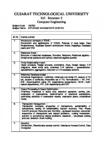
Record format description When you describe a database file to the system, you describe two major parts of the file: the record format and the access path. The record format describes the order of the fields in each record. The record format also describes each field in detail, including length, data type (for example, packed decimal or character), validity checks, text description, and other information. The following example shows the relationship between the record format and the records in a physical file:

In this example of specifications for record format ITMMST, there are three fields. Field ITEM is zoned decimal, 5 digits, with no decimal position. Field DESCRP is character, with 18 positions. Field PRICE is zoned decimal, 5 digits, with two decimal positions. A physical file can have only one record format. The record format in a physical file describes the way the data is actually stored. A logical file contains no data. Logical files are used to arrange data from one or more physical files into different formats and sequences. For example, a logical file can change the order of the fields in the physical file, or present to the program only some of the fields stored in the physical file. A logical file record format can change the length and data type of fields that are stored in physical files. The system does the necessary conversion between the physical file field description and the logical file field description. For example, a physical file can describe a field FLDA as a packed decimal field of 5 digits, and a logical file that uses FLDA might redefine it as a zoned decimal field of 7 digits. In this case, when your program uses the logical file to read a record, the system automatically converts (unpacks) FLDA to zoned decimal format.

6


Access path description An access path of a database file describes the order in which records are to be retrieved. When you describe an access path, you describe whether it is a keyed sequence access path or an arrival sequence access path. Related concepts “Describing access paths for database files” on page 83 An access path describes how records in a database file are retrieved. You can define the access path for a database file in various ways.

Naming conventions for a database file The file name, record format name, and field name can be as long as 10 characters and must follow all system naming conventions. Some high-level languages have more restrictive naming conventions than the system has. For example, the RPG/400® language allows only 6-character names, while the system allows 10-character names. In some cases, you can temporarily change (rename) the system name to one that meets the high-level language restrictions. For more information about renaming database fields in programs, see your high-level language topic collection. In addition, names must be unique as follows: v Field names must be unique in a record format. v Record format names and member names must be unique in a file. v File names must be unique in a library.

Database data protection and monitoring To ensure data integrity and consistency, you can enforce either business rules or data type rules. You can enforce business rules using the following methods: v Referential constraints let you put controls (constraints) on data in files you define as having a mutual dependency. A referential constraint lets you specify rules to be followed when changes are made to files with constraints. v Triggers let you run your own program to take any action or evaluate changes when files are changed. When predefined changes are made or attempted, a trigger program is run. The system performs data type checking in certain instances to ensure, for example, that data in a numeric field is really numeric.

| | |

In addition, the system protects data from loss using the following methods: v Journaling and commitment control functions v System-managed access path protection (SMAPP) support Related concepts “Ensuring data integrity with referential constraints” on page 253 You use referential constraints to enforce the referential integrity of your database. Referential integrity encompasses all of the mechanisms and techniques that you can use to ensure that your database contains only valid data. “Triggering automatic events in your database” on page 265 A trigger is a set of actions that run automatically when a specified change or read operation is performed on a specified database file. You can define a set of trigger actions in any high-level language that is supported on the i5/OS operating system. “Recovering and restoring your database” on page 224 You can use several i5/OS save and restore functions to recover your database after the system loses data. Database programming

7

Database file sizes Before you design and create a database file, you need to know the maximum size allowed for the file. The following table lists the maximum values for database files. Description

|

| | |

Maximum value

Number of bytes in a record 32 766 bytes Number of fields in a record format 8 000 fields Number of key fields in a file 120 fields Size of key for physical and logical files 32 768 characters1 Size of key for ORDER BY (SQL) and KEYFLD 10 000 bytes (OPNQRYF) Number of records contained in a file member 4 294 967 294 records2 Number of bytes in a file member 1 869 162 846 624 bytes3 Number of bytes in an access path 1 099 511 627 776 bytes3 5 Number of keyed logical files built over a physical file 3686 files member Number of physical file members in a logical file 32 members member Number of members that can be joined 256 members Size of a character or DBCS field 32 766 bytes4 Size of a zoned decimal or packed decimal field 63 digits Maximum number of distinct database files that can be ~500 000 in use at one time Maximum number of members in a physical or logical 32 767 file Maximum number of constraints per physical file 300 constraints Maximum number of triggers per physical file 300 triggers Maximum number of recursive insert and update trigger 200 calls 1 When a first-changed-first-out (FCFO) access path is specified for the file, the maximum value for the size of the key for physical and logical files is 32 763 for ACCPTHSIZ(*MAX1TB) and 1995 characters for ACCPTHSIZ(*MAX4GB).

| |

2

|

When ACCPTHSIZ(*MAX4GB) is specified, use the following formula:

| |

2,867,200,000 10 + (.8 x key length)

|

When ACCPTHSIZ(*MAX1TB) is specified, use the following formula:

| |

725,680,000,000 12 + (.8 x key length)

|

These are estimated values. The actual maximum number of records can vary significantly.

For files with keyed sequence access paths, the maximum number of records in a member varies and can be estimated using the following formulas.

3

Both the number of bytes in a file member and the number of bytes in an access path must be looked at when message CPF5272 is sent indicating that the maximum system object size has been reached. 4

The maximum size of a variable-length character or DBCS field is 32 740 bytes. DBCS-graphic field lengths are expressed in terms of characters; therefore, the maximums are 16 383 characters (fixed length) and 16 370 characters (variable length). 5

The maximum is 4 294 966 272 bytes if the access path is created with a maximum size of 4 gigabytes (GB), ACCPTHSIZ(*MAX4GB).

8


These are maximum values. There are situations where the actual limit you experience will be less than the stated maximum. For example, certain high-level languages can have more restrictive limits than those described above. Keep in mind that performance can suffer as you approach some of these maximums. For example, the more logical files you have built over a physical file, the greater the chance that system performance can suffer (if you are frequently changing data in the physical file that causes a change in many logical file access paths). Normally, an i5/OS database file can grow until it reaches the maximum size allowed on the operating system. The operating system normally does not allocate all the file space at once. Rather, it occasionally allocates additional space as the file grows larger. This method of automatic storage allocation provides the best combination of good performance and effective auxiliary storage space management. If you want to control the size of the file, the storage allocation, and whether the file should be connected to auxiliary storage, you can use the SIZE, ALLOCATE, and CONTIG parameters on the Create Physical File (CRTPF) and the Create Source Physical File (CRTSRCPF) commands. You can use the following formulas to estimate the disk size of your physical and logical files. v For a physical file (excluding the access path) that does not contain null-capable fields: | |

Disk size = (number of valid and deleted records + 1) x (record length + 1) + 20480 x (number of members) + 8192 The size of the physical file depends on the SIZE and ALLOCATE parameters on the CRTPF and CRTSRCPF commands. If you specify ALLOCATE(*YES), the initial allocation and increment size on the SIZE keyword must be used instead of the number of records. v For a physical file (excluding the access path) that contains null-capable fields:

| | | |

Disk size = (number of valid and deleted records + 1) x (record length + 1) + 20480 x (number of members) + 8192 + ((number of fields in format ÷ 8) rounded up) x (number of valid and deleted records + 1) The size of the physical file depends on the SIZE and ALLOCATE parameters on the CRTPF and CRTSRCPF commands. If you specify ALLOCATE(*YES), the initial allocation and increment size on the SIZE keyword must be used instead of the number of records. v For a logical file (excluding the access path):

|

Disk size = (12288) x (number of members) + 8192 v For a keyed sequence access path the generalized equation for index size, per member, is:

let a = (LimbPageUtilization - LogicalPageHeaderSize) * (LogicalPageHeaderSize - LeafPageUtilization - 2 * NodeSize) let b = NumKeys * (TerminalTextPerKey + 2 * NodeSize) * (LimbPageUtilization - LogicalPageHeaderSize + 2 * NodeSize) + CommonTextPerKey * [ LimbPageUtilization + LeafPageUtilization - 2 * (LogicalPageHeaderSize - NodeSize) ] - 2 * NodeSize * (LeafPageUtilization - LogicalPageHeaderSize + 2 * NodeSize) let c = CommonTextPerKey * [ 2 * NodeSize - CommonTextPerKey - NumKeys * (TerminalTextPerKey + 2 * NodeSize) ] Database programming

9

then NumberLogicalPages = ceil( [ -b - sqrt(b ** 2 - 4 * a * c) ] / (2 * a)) and TotalIndexSize = NumberLogicalPages * LogicalPageSize This equation is used for both three and four byte indexes by changing the set of constants in the equation as follows. Constant

Three-byte index

Four-byte index

NodeSize LogicalPageHeaderSize LimbPageUtilization LeafPageUtilization

3 16 .75 * LogicalPageSize .75 * LogicalPageSize

4 64 .75 * LogicalPageSize .80 * LogicalPageSize

The remaining constants, CommonTextPerKey and TerminalTextPerKey, are probably best estimated by using the following formulas:

CommonTextPerKey = [ min(max(NumKeys - 256,0),256) + min(max(NumKeys - 256 * 256,0),256 * 256) + min(max(NumKeys - 256 * 256 * 256,0), 256 * 256 * 256) + min(max(NumKeys - 256 * 256 * 256 * 256,0), 256 * 256 * 256 * 256) ] * (NodeSize + 1) / NumKeys TerminalTextPerKey = KeySizeInBytes - CommonTextPerKey This should reduce everything needed to calculate the index size to the type of index (that is, 3 or 4 byte), the total key size, and the number of keys. The estimate should be greater than the actual index size because the common text estimate is minimal. Given this generalized equation for index size, the LogicalPageSize is as follows. Table 1. LogicalPageSize values

| | | |

Key Length

*MAX4GB (3-byte) LogicalPageSize

*MAX1TB (4-byte) LogicalPageSize

1 - 500 501 - 1000 1001 - 2000 2001 - 10 000 10 001 - 18 000 18 001 - 26 000 26 001 - 32 768

4096 bytes 8192 bytes 16 384 bytes N/A N/A N/A N/A

8192 bytes 16 384 bytes 32 768 bytes 65 536 bytes 131 072 bytes 262 144 bytes 524 288 bytes

The LogicalPageSizes in Table 1 generate the following LimbPageUtilizations.

| | | |

Key Length

*MAX4GB (3-byte) LimbPageUtilization

*MAX1TB (4-byte) LimbPageUtilization

1 - 500 501 - 1000 1001 - 2000 2001 - 10 000 10 001 - 18 000 18 001 - 26 000 26 001 - 32 768



10


The LogicalPageSizes in Table 1 on page 10 generate the following LeafPageUtilizations.

| | | |

Key Length

*MAX4GB (3-byte) LeafPageUtilization

*MAX1TB (4-byte) LeafPageUtilization

1 - 500 501 - 1000 1001 - 2000 2001 - 10 000 10 001 - 18 000 18 001 - 26 000 26 001 - 32 768



Then to simplify the generalized equation for index size, let:

CommonTextPerKey = 0 which would cause: TerminalTextPerKey = KeySizeInBytes b = NumKeys * (KeySizeInBytes + 2 * NodeSize) * (LimbPageUtilization - LogicalPageHeaderSize + 2 * NodeSize) - 2 * NodeSize * (LeafPageUtilization - LogicalPageHeaderSize + 2 * NodeSize) c = 0 NumberLogicalPages = ceil( [ -b - sqrt(b ** 2 ) ] / (2 * a)) = ceil[ (-2 * b) / (2 * a) ] = ceil[ -b/a ]

Example: Database file sizes This example shows how to estimate the maximum size of a database file. A *MAX1TB (4-byte) access path with 120 byte keys and 500 000 records TotalIndexSize has a TotalIndexSize in bytes as follows: a = (LimbPageUtilization - LogicalPageHeaderSize) * (LogicalPageHeaderSize - LeafPageUtilization - 2 * NodeSize) = (6144 - 64) * (64 - 6554 - 2 * 4) = 6080 * -6498 = -39,507,840 b = NumKeys * (KeySizeInBytes + 2 * NodeSize) * (LimbPageUtilization - LogicalPageHeaderSize + 2 * NodeSize) - 2 * NodeSize * (LeafPageUtilization - LogicalPageHeaderSize + 2 * NodeSize) = 500,000 * (120 + 2 * 4) * (6144 - 64 + 2 * 4) - 2 * 4 * (6554 - 64 + 2 * 4) = 500,000 * 128 * 6088 - 8 * 6498 = 3.896319e+11 NumberLogicalPages = ceil[ -b/a ] = ceil[ -3.896319e+11/-39507840 ] Database programming

11

= 9863 TotalIndexSize = NumberLogicalPages * LogicalPageSize = 9863 * 8192 = 80,797,696 bytes

The equation for index size in previous versions of the operating system produces the following result: TotalIndexSize = (number of keys) * (key length + 8) * (0.8) * (1.85) + 4096 = (NumKeys) * (KeySizeInBytes + 8) * (0.8) * (1.85) + 4096 = 500000 * 128 * .8 * 1.85 + 4096 = 94,724,096

This estimate can differ significantly from your file. The keyed sequence access path depends heavily on the data in your records. The only way to get an accurate size is to load your data and display the file description. The following table shows a list of minimum file sizes. Description

Minimum size

Physical file without a member Physical file with a single member Keyed sequence access path

8192 bytes 20 480 bytes 12 288 bytes

Note: Additional space is not required for an arrival sequence access path. In addition to the file sizes, the system maintains internal formats and directories for database files. (These internal objects are owned by user profile QDBSHR.) The following are estimates of the sizes of those objects: v For any file not sharing another file’s format: Format size = (144 x number of fields) + 4096

|

v For files sharing their format with any other file: | |

Format sharing directory size = (16 x number of files sharing the format) + 4096 v For each physical file and each physical file member having a logical file or logical file member built over it:

| |

Data sharing directory size = (16 x number of files or members sharing data) + 4096 v For each file member having a logical file member sharing its access path: Access path sharing directory size = (16 x number of files or members sharing access path) + 4096

| |

Setting up database files You can create, define, and secure a database file using the traditional system interface or iSeries Navigator. Related concepts

12


“Traditional system interface” on page 3 The i5/OS traditional system interface is the full set of system commands and other non-SQL facilities that you can use to access and change DB2 Universal Database for iSeries data. Getting started with iSeries Navigator

Creating and describing database files You can create and describe a library and a database file using the traditional system interface. The system supports several methods for creating and describing a database file: v Interactive data definition utility (IDDU) You can create a database file by using IDDU, part of the WebSphere Development Studio for iSeries licensed program. If you are using IDDU to describe your database files, you might also consider using it to create your files. v Control language (CL), using the source entry utility (SEU) or the data file utility (DFU) to specify data description specifications (DDS) You can create a database file by using CL. The CL database file create commands are Create Physical File (CRTPF), Create Logical File (CRTLF), and Create Source Physical File (CRTSRCPF). After a database file is created, you can use SEU or DFU to describe data in the file. SEU and DFU are part of the IBM WebSphere Development Studio for iSeries licensed program. These topics focus on how to create files using these methods. v Structured Query Language (SQL) You can create and describe a database file (table) by using SQL statements. SQL is the IBM relational database language. It can be used to interactively describe and create database files. v iSeries Navigator You can also create a database file (table) using iSeries Navigator. Related concepts Creating a table Getting started with iSeries Navigator SQL programming “Traditional system interface” on page 3 The i5/OS traditional system interface is the full set of system commands and other non-SQL facilities that you can use to access and change DB2 Universal Database for iSeries data.

Creating a library A library is a system object that serves as a directory to other objects. A library groups related objects and allows you to find objects by name. To create a library, use iSeries Navigator or the Create Library (CRTLIB) command. The system-recognized identifier for the object type is *LIB. Before you can create a database file, you must create a library to store it. You can create a library in the following ways: v You can use iSeries Navigator to create a library (in SQL, called a schema). v You can use the Create Library (CRTLIB) command to create the library. When creating a library, you can specify the auxiliary storage pool (ASP) where the library is to be stored. This allows you to create multiple, separate databases.

Creating a library (schema) using iSeries Navigator To create a library (in SQL, called a schema) from iSeries Navigator, follow these steps: 1. From iSeries Navigator, expand the system you want to use. 2. Expand Databases and the database that you want to work with. Database programming

13

3. 4. 5. 6. 7. 8. 9.

Right-click Schemas and click New Schema. On the New Schema window, specify a schema name. To add this schema to the list of schemas displayed, select Add to displayed list of schemas. To create as a standard schema, select Create as a standard schema. To create a data dictionary, select Create a data dictionary. Specify a disk pool to contain the schema. Specify a description.

10. Click OK. Related reference Create Library (CRTLIB) command

Setting up source files You can either create a source file or use an IBM-supplied source file. Related concepts “Using source files” on page 240 DB2 Universal Database for iSeries provides a range of support for source files. Why source files are used: A source file contains input (source) data that is needed to create some types of objects. A source file is used when a command alone cannot provide sufficient information for creating an object. For example, to create a control language (CL) program, you must use a source file that contains source statements in the form of commands. To create a logical file, you must use a source file that contains data description specifications (DDS). To create the following objects, source files are required: v High-level language programs v Control language programs v Logical files v Intersystem communications function (ICF) files v Commands To create the following objects, source files can be used, but are not required: v Physical files v Display files v Printer files v Translate tables A source file can be a database file, a diskette file, a tape file, or an inline data file. (An inline data file is included as part of a job.) A source database file is another type of database file. You can use a source database file as you use any other database file on the system. Related concepts “Database files” on page 3 A database file is one of the several types of the system object type *FILE. A database file contains descriptions of how input data is to be presented to a program from internal storage and how output data is to be presented to internal storage from a program. Creating a source file:

14


Before creating a source file, you should first create a library. Then use the Create Source Physical File (CRTSRCPF), Create Physical File (CRTPF), or Create Logical File (CRTLF) command to create a source file. v Create Source Physical File (CRTSRCPF) command Normally, you use the CRTSRCPF command to create a source file, because many of the parameters default to values that you usually want for a source file. v Create Physical File (CRTPF), or Create Logical File (CRTLF) command If you want to create a source file and define the record format and fields using data description specifications (DDS), use the Create Physical File (CRTPF) or Create Logical File (CRTLF) command. As an alternative to creating a source file, you can use source files supplied with the i5/OS and other licensed programs. Related concepts “Creating a library” on page 13 A library is a system object that serves as a directory to other objects. A library groups related objects and allows you to find objects by name. To create a library, use iSeries Navigator or the Create Library (CRTLIB) command. Related reference Create Physical File (CRTPF) command Create Logical File (CRTLF) command Creating a source file using the Create Source Physical File (CRTSRCPF) command: You can create a source file using the default values of the Create Source Physical File (CRTSRCPF) command. CRTSRCPF FILE(QGPL/FRSOURCE) TEXT(’Source file’)

The CRTSRCPF command creates a physical file, but with attributes appropriate for source physical files. For example, the default record length for a source file is 92 (80 for the source data field, 6 for the source sequence number field, and 6 for the source date field). Related reference Create Source Physical File (CRTSRCPF) command Creating a source file with DDS: If you want to create a source file with data description specifications (DDS), use the Create Physical File (CRTPF) or Create Logical File (CRTLF) command. If you want to create a source file for which you need to define the record format, use the CRTPF or CRTLF command. If you create a source logical file, the logical file member should only refer to one physical file member to avoid duplicate keys. The following example shows the DDS needed to define the record format for a source file using the CRTPF command: |...+....1....+....2....+....3....+....4....+....5....+....6....+....7....+....8 A* R RECORD1 A F1 6S 2 A F2 6S A F3 92A

Related reference Create Physical File (CRTPF) command Create Logical File (CRTLF) command


15

Creating a source file without DDS: When you create a source physical file without using DDS, but by specifying the record length (RCDLEN parameter) on the Create Source Physical File (CRTSRCPF) command, the source created contains three fields: SRCSEQ, SRCDAT, and SRCDTA. The record length must include 12 characters for sequence number and date-of-last-change fields so that the length of the data portion of the record equals the record length minus 12. The data portion of the record can be defined to contain more than one field (each of which must be character or zoned decimal). If you want to define the data portion of the record as containing more than one field, you must define the fields using DDS. A record format that consists of the following three fields is automatically used for a source physical file that is created with the CRTSRCPF command. Field

Name

Data type and length

Description

1

SRCSEQ

Sequence number for record

2

SRCDAT

3

SRCDTA

Zoned decimal, 6 digits, 2 decimal positions Zoned decimal, 6 digits, no decimal positions Character, any length

Date of last update of record Data portion of the record (text)

Note: For all IBM-supplied database source files, the length of the data portion is 80 bytes. For IBM-supplied device source files, the length of the data portion is the maximum record length for the associated device. IBM-supplied source files: For your convenience, the i5/OS licensed program and other licensed programs provide a database source file for each type of source. This table shows these IBM-supplied source files. ||

File name

Library name

Used to create

| | | | | | | | | | | | | | | | | | | | |

QCBLLESRC QCBLSRC

QGPL QGPL

QCLSRC QCMDSRC QCPPSRC QCSRC QDDSSRC QFMTSRC QLBLSRC QPLISRC QPNLSRC

QGPL QGPL QGPL QGPL QGPL QGPL QGPL QGPL QGPL

QREXSRC QRPGLESRC QRPGSRC

QGPL QGPL QGPL

QS36PRC

#LIBRARY

QS36SRC

#LIBRARY

ILE COBOL programs System/38™ compatible COBOL programs CL programs Command definition statements C++ programs C programs Files definition statements Sort source COBOL/400® programs PL/I programs Panel group (UIM) definition statements REXX procedures ILE RPG programs RPG/400 and System/38 compatible RPG programs System/36™ compatible COBOL and RPG II procedures System/36 compatible COBOL and RPG programs

16


|

File name

Library name

Used to create

| | |

QTBLSRC QTXTSRC

QGPL QGPL

Translation tables Text

| | | | | | |

You can either add your source members to these files or create your own source files. Normally, you want to create your own source files using the same names as the IBM-supplied files, but in different libraries. The IBM-supplied source files are created with the file names used for the corresponding create command (for example, the Create CL Program (CRTCLPGM) command uses the QCLSRC file name as the default). Additionally, the IBM-supplied programmer menu uses the same default names. (If you use the same file names as the IBM-supplied names, ensure that the library containing your source files precedes the library containing the IBM-supplied source files in the library list.) Source file attributes: Here are the attributes common to most source files and the restrictions on using these attributes. Source files usually have the following attributes: v A record length of 92 characters (this includes a 6-byte sequence number, a 6-byte date, and 80 bytes of source). v Keys (sequence numbers) that are unique even though the access path does not specify unique keys. You are not required to specify a key for a source file. Default source files are created without keys (arrival sequence access path). A source file created with an arrival sequence access path requires less storage space and reduces save/restore time in comparison to a source file for which a keyed sequence access path is specified. v More than one member. v Member names that are the same as the names of the objects that are created using them. v The same record format for all records. v Relatively few records in each member compared to most data files. Some restrictions are: v The source sequence number must be used as a key, if a key is specified. v The key, if one is specified, must be in ascending sequence. v The access path cannot specify unique keys. v The ALTSEQ keyword is not allowed in data description specifications (DDS) for source files. v The first field must be a 6-digit sequence number field containing zoned decimal data and two decimal digits. v The second field must be a 6-digit date field containing zoned decimal data and zero decimal digits. v All fields following the second field must be zoned decimal or character.

Describing database files You can use several methods to describe i5/OS database files. This topic discusses how to describe a database file with data description specifications (DDS) because DDS has the most options for defining data. If you want to describe a file just to the record level, you can use the record length (RCDLEN) parameter on the Create Physical File (CRTPF) and Create Source Physical File (CRTSRCPF) commands. If you want to describe your file to the field level, several methods can be used to describe data to the database system: interactive data definition utility (IDDU), Structured Query Language (SQL) commands, or data description specifications (DDS). Interactive data definition utility (IDDU)


17

Physical files can be described with IDDU. You might use IDDU because it is a menu-driven, interactive method of describing data. You might be familiar with describing data using IDDU in a System/36 environment. In addition, IDDU allows you to describe multiple-format physical files for use with Query, iSeries Access, and the data file utility (DFU). When you use IDDU to describe your files, the file definition becomes part of the i5/OS data dictionary. DB2 Universal Database for iSeries Structured Query Language (SQL) SQL can be used to describe a database file. It supports statements to describe the fields in the database file and to create the file. SQL was created by IBM to meet the need for a standard and common database language. It is currently used on all IBM DB2 platforms and on many other database implementations from many different manufacturers. When you create a database file using the DB2 UDB for iSeries SQL, the file description is automatically added to a data dictionary in the SQL collection. The data dictionary (or catalog) is then automatically maintained by the system. SQL is the language of choice for accessing databases on many other platforms. It is the only language for distributed databases and heterogeneous systems. Data description specifications (DDS) Externally described files can be described with DDS. DDS provides descriptions of the field-level, record-level, and file-level information. You might use DDS because it provides the most options for the programmer to describe data in the database. For example, only with DDS can you describe key fields in logical files. The DDS form provides a common format for describing data externally. DDS data is column sensitive. The examples that follow have numbered columns and show the data in the correct columns. After a database file is described, you can view the description. Related concepts IDDU Use PDF SQL programming SQL reference “Displaying information about database files” on page 214 Using iSeries Navigator and CL commands, you can display various types of information about database files. Describing database files using DDS: When you describe a database file using data description specifications (DDS), you can describe the file at the file, record-format, join, field, key-field, and select/omit-field levels. v File-level DDS provides the system information about the entire file. For example, you can specify whether all the key field values in the file must be unique. v Record format-level DDS provides the system information about a specific record format in the file. For example, when you describe a logical file record format, you can specify the physical file that it is based on. v Join-level DDS provides the system information about the physical files that are used in a join logical file. For example, you can specify how to join two physical files. v Field-level DDS provides the system information about individual fields in the record format. For example, you can specify the name and attributes of each field.

18


v Key field-level DDS provides the system information about the key fields for the file. For example, you can specify which fields in the record format are to be used as key fields. v Select/omit field-level DDS provides the system information about which records are to be returned to the program during file processing. Select/omit specifications apply to logical files only. Related concepts DDS for physical and logical files Example: Describing a physical file using DDS: This example shows how to describe a physical file using DDS. The DDS for a physical file, as shown in the next example, must be in the following order: 1

File-level entries (optional). The UNIQUE keyword is used to indicate that the value of the key field in each record in the file must be unique. Duplicate key values are not allowed in this file.

2

Record format-level entries. The record format name is specified, along with an optional text description.

3

Field-level entries. The field names and field lengths are specified, along with an optional text description for each field.

4

Key field-level entries (optional). The field names used as key fields are specified.

5

Comment (optional).

|...+....1....+....2....+....3....+....4....+....5....+....6....+....7....+....8 A* ORDER HEADER FILE (ORDHDRP) A 5 A 1 UNIQUE A 2 R ORDHDR TEXT(’Order header record’) A 3 CUST 5 0 TEXT(’Customer number’) A ORDER 5 0 TEXT(’Order number’) A . A . A . A K CUST A 4 K ORDER

The following example shows a physical file ORDHDRP (an order header file), with an arrival sequence access path without key fields specified, and the DDS necessary to describe that file. Record format of physical file ORDHDRP Customer number (CUST) — Packed decimal length 5, No decimals Order number (ORDER) — Packed Decimal Length 5, No decimals Order date (ORDATE) — Packed decimal length 6, No decimals Purchase order number (CUSORD) — Packed decimal length 15, No decimals Shipping instructions (SHPVIA) — Character length 15 Order status (ORDSTS) — Character length 1 ... State (STATE) — Character length 2 |...+....1....+....2....+....3....+....4....+....5....+....6....+....7....+....8 A* ORDER HEADER FILE (ORDHDRP) A R ORDHDR TEXT(’Order header record’) A CUST 5 0 TEXT(’Customer Number’) A ORDER 5 0 TEXT(’Order Number’) A ORDATE 6 0 TEXT(’Order Date’) Database programming

19

A A A A A A A A A A A A A A A

CUSORD SHPVIA ORDSTS OPRNME ORDAMT CUTYPE INVNBR PRTDAT SEQNBR OPNSTS LINES ACTMTH ACTYR STATE

15 15 1 10 9 1 5 6 5 1 3 2 2 2

0

2 0 0 0 0 0 0

TEXT(’Customer Order No.’) TEXT(’Shipping Instr’) TEXT(’Order Status’) TEXT(’Operator Name’) TEXT(’Order Amount’) TEXT(’Customer Type’) TEXT(’Invoice Number’) TEXT(’Printed Date’) TEXT(’Sequence Number’) TEXT(’Open Status’) TEXT(’Order Lines’) TEXT(’Accounting Month’) TEXT(’Accounting Year’) TEXT(’State’)

The R in position 17 indicates that a record format is being defined. The record format name ORDHDR is specified in positions 19 through 28. You make no entry in position 17 when you are describing a field; a blank in position 17 along with a name in positions 19 through 28 indicates a field name. The data type is specified in position 35. The valid data types are: Entry

Meaning

A

Character

P

Packed decimal

S

Zoned decimal

B

Binary

F

Floating point

H

Hexadecimal

L

Date

T

Time

Z

Timestamp

Notes: 1. For double-byte character set (DBCS) data types, see “Double-byte character set considerations” on page 291. 2. The system performs arithmetic operations more efficiently for the packed-decimal than for the zoned-decimal data type. 3. Some high-level languages do not support floating-point data. 4. Some special considerations that apply when you are using floating-point fields are: v The precision associated with a floating-point field is a function of the number of bits (single or double precision) and the internal representation of the floating-point value. This translates into the number of decimal digits supported in the significant and the maximum values that can be represented in the floating-point field. v When a floating-point field is defined with fewer digits than supported by the precision specified, that length is only a presentation length and has no effect on the precision used for internal calculations. v Although floating-point numbers are accurate to 7 (single) or 15 (double) decimal digits of precision, you can specify up to 9 or 17 digits. You can use the extra digits to uniquely

20


establish the internal bit pattern in the internal floating-point format so identical results are obtained when a floating-point number in internal format is converted to decimal and back again to internal format. If the data type (position 35) is not specified, the decimal positions entry is used to determine the data type. If the decimal positions (positions 36 through 37) are blank, the data type is assumed to be character (A); if these positions contain a number 0 through 31, the data type is assumed to be packed decimal (P). The length of the field is specified in positions 30 through 34, and the number of decimal positions (for numeric fields) is specified in positions 36 and 37. If a packed or zoned decimal field is to be used in a high-level language program, the field length must be limited to the length allowed by the high-level language you are using. The length is not the length of the field in storage but the number of digits or characters specified externally from storage. For example, a 5-digit packed decimal field has a length of 5 specified in DDS, but it uses only 3 bytes of storage. Character or hexadecimal data can be defined as variable length by specifying the VARLEN field-level keyword. Generally you would use variable length fields, for example, as an employee name within a database. Names usually can be stored in a 30-byte field; however, there are times when you need 100 bytes to store a very long name. If you always define the field as 100 bytes, you waste storage. If you always define the field as 30 bytes, some names are truncated. You can use the DDS VARLEN keyword to define a character field as variable length. You can define this field as: v Variable-length with no allocated length. This allows the field to be stored using only the number of bytes equal to the data (plus two bytes per field for the length value and a few overhead bytes per record). However, performance might be affected because all data is stored in the variable portion of the file, which requires two disk read operations to retrieve. v Variable-length with an allocated length equal to the most likely size of the data. This allows most field data to be stored in the fixed portion of the file and minimizes unused storage allocations common with fixed-length field definitions. Only one read operation is required to retrieve field data with a length less than the allocated field length. Field data with a length greater than the allocated length is stored in the variable portion of the file and requires two read operations to retrieve the data. Example: Describing a logical file using DDS: This example shows how to describe a logical file using DDS. The DDS for a logical file, as shown in the next example, must be in the following order: 1

File-level entries (optional). In this example, the UNIQUE keyword indicates that for this file the key value for each record must be unique; no duplicate key values are allowed.

For each record format: 2

Record format-level entries. In this example, the record format name, the associated physical file, and an optional text description are specified.

3

Field-level entries (optional). In this example, each field name used in the record format is specified.

4

Key field-level entries (optional). In this example, the Order field is used as a key field.

5

Select/omit field-level entries (optional). In this example, all records whose Opnsts field contains a value of N are omitted from the file’s access path. That is, programs reading records from this file never see a record whose OPNSTS field contains an N value.

6

Comment. Database programming

21

|...+....1....+....2....+....3....+....4....+....5....+....6....+....7....+....8 A* ORDER HEADER FILE (ORDHDRP) A 6 A 1 UNIQUE A 2 R ORDHDR PFILE(ORDHDRP) A 3 ORDER TEXT(’Order number’) A CUST TEXT(’Customer number’) A . A . A . A 4 K ORDER A O OPNSTS 5 CMP(EQ ’N’) A S ALL

A logical file must be created after all physical files on which it is based are created. The PFILE keyword in this example is used to specify the physical file or files on which the logical file is based. Record formats in a logical file can be: v A new record format based on fields from a physical file v The same record format as in a previously described physical or logical file. Fields in the logical file record format must either appear in the record format of at least one of the physical files or be derived from the fields of the physical files on which the logical file is based. Related concepts “Sharing existing record format descriptions in a database file” on page 25 A record format can be described once in either a physical or a logical file (except a join logical file) and can be used by many files. When you describe a new file, you can specify that the record format of an existing file is to be used by the new file. “Setting up logical files” on page 39 A logical file contains no data, but it defines record formats for one or more physical files. You can create various logical files and describe their record formats and access paths using data description specifications (DDS). Control language Additional DDS field definition functions: You can describe additional information about the fields in the physical and logical file record formats with function keywords (positions 45 through 80 on the DDS form). Some of the things you can specify include: v Validity checking keywords to verify that the field data meets your standards. For example, you can describe a field to have a valid range of 500 to 900. (This checking is done only when data is typed on a keyboard to the display.) v Editing keywords to control how a field should be displayed or printed. For example, you can use the EDTCDE(Y) keyword to specify that a date field is to appear as MM/DD/YY. The EDTCDE and EDTWRD keywords can be used to control editing. (This editing is done only when used in a display or printer file.) v Documentation, heading, and name control keywords to control the description and name of a field. For example, you can use the TEXT keyword to document a description of each field. This text description is included in your compiler list to better document the files used in your program. The TEXT and COLHDG keywords control text and column-heading definitions. The ALIAS keyword can be used to provide a more descriptive name for a field. The alias, or alternative name, is used in a program (if the high-level language supports alias names). v Content and default value keywords to control the null content and default data for a field. The ALWNULL keyword specifies whether a null value is allowed in the field. If ALWNULL is used, the default value of the field is null. If ALWNULL is not present at the field level, the null value is not

22


allowed, character and hexadecimal fields default to blanks, and numeric fields default to zeros, unless the DFT (default) keyword is used to specify a different value. Using existing field descriptions and field reference files to describe a database file: If you want to use a field description in an existing file, you can copy that field description into your new file description. You can also create a field reference file to contain the field descriptions that you need for any group of files. DDS keywords REF and REFFLD allow you to refer to a field description in an existing file. This helps reduce the effort of coding DDS statements. It also helps ensure that the field attributes are used consistently in all files that use the field. In addition, you can create a physical file for the sole purpose of using its field descriptions. That is, the file does not contain data; it is used only as a reference for the field descriptions for other files. This type of file is known as a field reference file. A field reference file is a physical file containing no data, just field descriptions. You can use a field reference file to simplify record format descriptions and to ensure that field descriptions are used consistently. You can create a field reference file using DDS and the Create Physical File (CRTPF) command. After the field reference file is created, you can build physical file record formats from this file without describing the characteristics of each field in each file. When you build physical files, all you need to do is to refer to the field reference file (using the REF and REFFLD keywords) and specify any changes. Any changes to the field descriptions and keywords specified in your new file override the descriptions in the field reference file. In the following example, a field reference file named DSTREFP is created for distribution applications. The following example shows the DDS needed to describe DSTREFP. |...+....1....+....2....+....3....+....4....+....5....+....6....+....7....+....8 A* FIELD REFERENCE FILE (DSTREFP) A R DSTREF TEXT(’Field reference file’) A A* FIELDS DEFINED BY CUSTOMER MASTER RECORD (CUSMST) A CUST 5 0 TEXT(’Customer numbers’) A COLHDG(’CUSTOMER’ ’NUMBER’) A NAME 20 TEXT(’Customer name’) A ADDR 20 TEXT(’Customer address’) A A CITY 20 TEXT(’Customer city’) A A STATE 2 TEXT(’State abbreviation’) A CHECK(MF) A CRECHK 1 TEXT(’Credit check’) A VALUES(’Y’ ’N’) A SEARCH 6 0 TEXT(’Customer name search’) A COLHDG(’SEARCH CODE’) A ZIP 5 0 TEXT(’Zip code’) A CHECK(MF) A CUTYPE 15 COLHDG(’CUSTOMER’ ’TYPE’) A RANGE(1 5) A A* FIELDS DEFINED BY ITEM MASTER RECORD (ITMAST) A ITEM 5 TEXT(’Item number’) A COLHDG(’ITEM’ ’NUMBER’) A CHECK(M10) A DESCRP 18 TEXT(’Item description’) A PRICE 5 2 TEXT(’Price per unit’) A EDTCDE(J) A CMP(GT 0) Database programming

23

A A A A A A A A A A A A A A* A A A A A A A A A A A A A A A A A A A A A A A A A A A A A A A* A A A A A A A A A A* A A A A* A A

ONHAND

5

WHSLOC

3

ALLOC

0

R

COLHDG(’PRICE’) TEXT(’On hand quantity’) EDTCDE(Z) CMP(GE 0) COLHDG(’ON HAND’) TEXT(’Warehouse location’) CHECK(MF) COLHDG(’BIN NO’) REFFLD(ONHAND *SRC) TEXT(’Allocated quantity’) CMP(GE 0) COLHDG(’ALLOCATED’)

FIELDS DEFINED BY ORDER HEADER RECORD (ORDHDR) ORDER 5 0 TEXT(’Order number’) COLHDG(’ORDER’ ’NUMBER’) ORDATE 6 0 TEXT(’Order date’) EDTCDE(Y) COLHDG(’DATE’ ’ORDERED’) CUSORD 15 TEXT(’Cust purchase ord no.’) COLHDG(’P.O.’ ’NUMBER’) SHPVIA 15 TEXT(’Shipping instructions’) ORDSTS 1 TEXT(’Order status code’) COLHDG(’ORDER’ ’STATUS’) OPRNME R REFFLD(NAME *SRC) TEXT(’Operator name’) COLHDG(’OPERATOR NAME’) ORDAMT 9 2 TEXT(’Total order value’) COLHDG(’ORDER’ ’AMOUNT’) INVNBR 5 0 TEXT(’Invoice number’) COLHDG(’INVOICE’ ’NUMBER’) PRTDAT 6 0 EDTCDE(Y) COLHDG(’PRINTED’ ’DATE’) SEQNBR 5 0 TEXT(’Sequence number’) COLHDG(’SEQ’ ’NUMBER’) OPNSTS 1 TEXT(’Open status’) COLHDG(’OPEN’ ’STATUS’) LINES 3 0 TEXT(’Lines on invoice’) COLHDG(’TOTAL’ ’LINES’) ACTMTH 2 0 TEXT(’Accounting month’) COLHDG(’ACCT’ ’MONTH’) ACTYR 2 0 TEXT(’Accounting year’) COLHDG(’ACCT’ ’YEAR’) FIELDS DEFINED BY ORDER DETAIL/LINE ITEM RECORD (ORDDTL) LINE 3 0 TEXT(’Line no. this item’) COLHDG(’LINE’ ’NO’) QTYORD 3 0 TEXT(’Quantity ordered’) COLHDG(’QTY’ ’ORDERED’ CMP(GE 0) EXTENS 6 2 TEXT(’Ext of QTYORD x PRICE’) EDTCDE(J) COLHDG(’EXTENSION’) FIELDS DEFINED BY ACCOUNTS RECEIVABLE ARBAL 8 2 TEXT(’A/R balance due’) EDTCDE(J) WORK AREAS AND OTHER FIELDS THAT OCCUR IN MULTIPLE PROGRAMS STATUS 12 TEXT(’status description’) A

Assume that the DDS in the previous example is entered into a source file FRSOURCE; the member name is DSTREFP. To create a field reference file, use the CRTPF command as follows:

24


CRTPF FILE(DSTPRODLB/DSTREFP) SRCFILE(QGPL/FRSOURCE) MBR(*NONE) TEXT(’Distribution field reference file’)

The parameter MBR(*NONE) tells the system not to add a member to the file (because the field reference file never contains data and therefore does not need a member). To describe the physical file ORDHDRP by referring to DSTREFP, use the following DDS example: |...+....1....+....2....+....3....+....4....+....5....+....6....+....7....+....8 A* ORDER HEADER FILE (ORDHDRP) - PHYSICAL FILE RECORD DEFINITION A REF(DSTREFP) A R ORDHDR TEXT(’Order header record’) A CUST R A ORDER R A ORDATE R A CUSORD R A SHPVIA R A ORDSTS R A OPRNME R A ORDAMT R A CUTYPE R A INVNBR R A PRTDAT R A SEQNBR R A OPNSTS R A LINES R A ACTMTH R A ACTYR R A STATE R A

The REF keyword (positions 45 through 80) with DSTREFP (the field reference file name) specified indicates the file from which field descriptions are to be used. The R in position 29 of each field indicates that the field description is to be taken from the reference file. When you create the ORDHDRP file, the system uses the DSTREFP file to determine the attributes of the fields included in the ORDHDR record format. To create the ORDHDRP file, use the CRTPF command. Assume that the DDS in the previous example was entered into a source file QDDSSRC; the member name is ORDHDRP. CRTPF FILE(DSTPRODLB/ORDHDRP) TEXT(’Order Header physical file’)

Note: The files used in some of the examples in this topic collection refer to this field reference file. Using a data dictionary for field reference in a database file: You can use a data dictionary and the interactive data description utility (IDDU) as an alternative to using a DDS field reference file. IDDU allows you to define fields in a data dictionary. Related concepts IDDU Use PDF Sharing existing record format descriptions in a database file: A record format can be described once in either a physical or a logical file (except a join logical file) and can be used by many files. When you describe a new file, you can specify that the record format of an existing file is to be used by the new file. Sharing existing record format descriptions can help reduce the number of DDS statements that you normally code to describe a record format in a new file and can save auxiliary storage space. Database programming

25

The file originally describing the record format can be deleted without affecting the files sharing the record format. After the last file using the record format is deleted, the system automatically deletes the record format description. The following example shows the DDS for two files. The first file describes a record format, and the second file shares the record format of the first file: |...+....1....+....2....+....3....+....4....+....5....+....6....+....7....+....8 A R RECORD1 PFILE(CUSMSTP) A CUST A NAME A ADDR A SEARCH A K CUST A |...+....1....+....2....+....3....+....4....+....5....+....6....+....7....+....8 A R RECORD1 PFILE(CUSMSTP) A FORMAT(CUSMSTL) A K NAME A

The first example shows file CUSMSTL, in which the fields Cust, Name, Addr, and Search make up the record format. The Cust field is specified as a key field. The DDS in the second example shows file CUSTMSTL1, in which the FORMAT keyword names CUSMSTL to supply the record format. The record format name must be RECORD1, the same as the record format name shown in the first example. Because the files are sharing the same format, both files have fields Cust, Name, Addr, and Search in the record format. In file CUSMSTL1, a different key field, Name is specified. The following restrictions apply to shared record formats: v A physical file cannot share the format of a logical file. v A join logical file cannot share the format of another file, and another file cannot share the format of a join logical file. v A view cannot share the format of another file, and another file cannot share the format of a view. (In the Structured Query Language (SQL), a view is an alternative representation of data from one or more tables. It can include all or some of the columns contained in the table or tables on which it is defined.) If the original record format is changed by deleting all related files and creating the original file and all the related files again, it is changed for all files that share it. If only the file with the original format is deleted and re-created with a new record format, all files previously sharing that file’s format continue to use the original format. If a logical file is defined but no field descriptions are specified and the FORMAT keyword is not specified, the record format of the first physical file (specified first on the PFILE keyword for the logical file) is automatically shared. The record format name specified in the logical file must be the same as the record format name specified in the physical file. To find out if a file shares a format with another file, use the RCDFMT parameter on the Display Database Relations (DSPDBR) command. Record format relationships between physical and logical files: When you change, add, or delete fields with the Change Physical File (CHGPF) command, a certain relationship exists between the physical and logical files that share the same record format. v When you change the length of a field in a physical file, you also change the length of the logical file’s field.

26


v When you add a field to the physical file, the field is also added to the logical file. v When you delete a field in the physical file, the field is also deleted from the logical file unless there is another dependency in DDS, such as a keyed field or a select/omit statement. Record format sharing limitation with physical and logical files: You might encounter this record format sharing limitation when you are duplicating the same database object multiple times. A record format can only be shared by 32KB objects. Error messages are issued when you reach this limitation. Note: Format sharing is performed for files that are duplicated. The format is shared up to 32 767 times. Beyond 32 767 times, if a file that shares the format is duplicated, a new format is created for the duplicated file. Specifying database file and member attributes: When you create a database file, database attributes are stored with the file and members. You specify attributes with database command parameters. Related reference Create Physical File (CRTPF) command Create Logical File (CRTLF) command Create Source Physical File (CRTSRCPF) command Add Physical File Member (ADDPFM) command Add Logical File Member (ADDLFM) command Change Physical File (CHGPF) command Change Physical File Member (CHGPFM) command Change Logical File (CHGLF) command Change Logical File Member (CHGLFM) command Change Source Physical File (CHGSRCPF) command Specifying the file name and member name (FILE and MBR) parameters: The FILE and MBR parameters specify the names of a database file and a file member. You name a file with the FILE parameter on a create command. You also name the library where the file is stored. When you create a physical or logical file, the system normally creates a member with the same name as the file. You can, however, specify a member name with the MBR parameter on a create command. You can also choose not to create any members by specifying MBR(*NONE). Note: The system does not automatically create a member for a source physical file. Specifying the physical file data members (DTAMBRS) parameter: The DTAMBRS parameter on the Create Logical File (CRTLF) command specifies the physical files and members that contain the data associated with a logical file member. You can specify: v The order in which the physical file members are to be read. v The number of physical file members to be used. Related concepts Database programming

27

“Defining logical file members” on page 44 You can define members in a logical file to separate the data into logical groups. A logical file member can be associated with one or several physical file members. Specifying the source file and source member (SRCFILE and SRCMBR) parameters: The SRCFILE and SRCMBR parameters specify the names of the source file and the source file member that contain DDS statements. If you do not specify a name: v The default source file name is QDDSSRC. v The default member name is the name specified on the FILE parameter. Specifying the file type (FILETYPE) parameter: The FILETYPE parameter specifies the type of database file. A database file type is either data (*DATA) or source (*SRC). The Create Physical File (CRTPF) and Create Logical File (CRTLF) commands use the default data file type (*DATA). Specifying the maximum number of members (MAXMBRS) parameter: The MAXMBRS parameter specifies the maximum number of members that a database file can hold. The default maximum number of members for physical and logical files is one, and the default for source physical files is *NOMAX. Specifying the preferred storage unit (UNIT) parameter: The system finds a place for a database file on auxiliary storage. The UNIT parameter specifies where to store the file. Note: Effective for Version 3 Release 6 the UNIT parameter is a no-operation (NOP) function for the following commands: v Create Physical File (CRTPF) v Create Logical File (CRTLF) v Create Source Physical File (CRTSRCPF) v Change physical File (CHGPF) v Change Logical File (CHGLF) v Change Source Physical File (CHGSRCPF) The parameter can still be coded; its presence does not cause an error. It will be ignored. The UNIT parameter specifies: v The location of data records in physical files. v The access path for both physical files and logical files. The data is placed on different units if: v There is not enough space on the unit. v The unit is not valid for your system. An informational message indicating that the file was not placed on the requested unit is sent when file members are added. (A message is not sent when the file member is extended.)

28


UNIT parameter tips In general, you should not specify the UNIT parameter. Let the system place the file on the disk unit of its choosing. This is usually better for performance, and relieves you of the task of managing auxiliary storage. If you specify a unit number and also an auxiliary storage pool, the unit number is ignored. Related concepts Independent disk pools examples Specifying the force write ratio (FRCRATIO) parameter: The FRCRATIO parameter on the create, change, or override database file command controls when database file changes are written to auxiliary storage. Normally, the system determines when to write changed data from main storage to auxiliary storage. Closing the file (except for a shared close) and the force-end-of-data operation forces remaining updates, deletions, and additions to auxiliary storage. If you are journaling the file, the FRCRATIO parameter should normally be *NONE. FRCRATIO parameter tip Using the FRCRATIO parameter has performance and recovery considerations for your system. Related concepts “Recovering and restoring your database” on page 224 You can use several i5/OS save and restore functions to recover your database after the system loses data. Specifying the force keyed access path (FRCACCPTH) parameter: The FRCACCPTH parameter controls whether access path changes are forced to auxiliary storage along with the associated records in a database file. FRCACCPTH (*YES) forces access path changes to auxiliary storage whenever the access path is changed. This reduces the chance that the access path needs rebuilding if the system fails. FRCACCPTH parameter tips Specifying FRCACCPTH(*YES) can degrade performance when changes occur to the access path. An alternative to forcing the access path is journaling the access path. Related concepts “Recovering and restoring your database” on page 224 You can use several i5/OS save and restore functions to recover your database after the system loses data. Specifying the record format level check (LVLCHK) parameter: When a database file is opened, the system can check whether the file definition is changed. The LVLCHK parameter specifies the check for record format description changes. When the file changes to an extent that your program might not be able to process the file, the system notifies your program. The default is to do level checking. You can specify if you want level checking when you: v Create a file. v Use a change database file command.


29

You can override the system and ignore the level check using the Override with Database File (OVRDBF) command. Example: Record format level check Assume that you compiled your program two months ago. At that time, the file was defined as having three fields in each record. Last week another programmer decided to add a field to the record format, so now each record has four fields. When your program tries to open the file, the system notifies your program that a significant change has occurred to the file definition since the last time the program was compiled. This notification is known as a record format level check. Specifying the access path maintenance (MAINT) parameter: | The MAINT parameter specifies the type of access path maintenance for all members of a database file. | | | |

If a file member is open, the system maintains the access path for the member when changes are made to the data in it. However, because more than one access path might exist for the same data, changing data in one file member might cause changes in the access paths for other file members that are not open (in use).

| | | | | | | | |

Here are the ways you can maintain access paths for all members of a database file: v Immediate maintenance of an access path means that the access path is maintained for a file member whenever changes are made to its associated data, whether the member is open or not. Access paths used by referential constraints are always in immediate maintenance. v Rebuild maintenance of an access path means that the access path is maintained for a file member only when the member is open, not when the member is closed; the access path is rebuilt when the member is opened the next time. When a file member with rebuild maintenance is closed, the system stops maintaining the access path. When the file member is opened again, the access path is totally rebuilt. If one or more programs have opened a specific file member with rebuild maintenance specified, the system maintains the access path for the member until the last user closes it. v Delayed maintenance of an access path means that any maintenance of the access path is done after the file member is opened the next time and when it remains open. However, the access path is not rebuilt as it is with rebuild maintenance. Changes to the access path are collected from the time the member is closed until it is opened again. When it is opened, only the collected changes are merged into the access path. If you do not specify the type of maintenance for a file, the default is immediate maintenance. MAINT parameter comparison: This table compares the effect of the immediate, rebuild, and delayed maintenance of access paths on opening and processing files. Function

Immediate maintenance

Rebuild maintenance

Delayed maintenance

Open

Fast open because the access path is current.

Slow open because access path must be rebuilt.

Moderately fast open because the access path does not have to be rebuilt, but it must still be changed. Slow open if extensive changes are needed.

30


Function

Immediate maintenance

Rebuild maintenance

Delayed maintenance

Process

Slower update and output operations when many access paths with immediate maintenance are built over changing data (the system must maintain the access paths).

Faster update and output operations when many access paths with rebuild maintenance are built over changing data and are not open (the system does not have to maintain the access paths).

Moderately fast update and output operations when many access paths with delayed maintenance are built over changing data and are not open (the system records the changes, but the access path itself is not maintained).

Notes: 1. Delayed or rebuild maintenance cannot be specified for a file that has unique keys. 2. Rebuild maintenance cannot be specified for a file if its access path is being journaled.

MAINT parameter tips: The type of access path maintenance to specify depends on the number of records and the frequency of add, delete, or update operations on the file when it is closed. You should use delayed maintenance for files that have relatively few changes to the access paths while the file members are closed. Delayed maintenance reduces system overhead by reducing the number of access paths that are maintained immediately. It might also result in faster open processing, because the access paths do not have to be rebuilt. You might want to specify immediate maintenance for access paths that are used frequently, or when you cannot wait for an access path to be rebuilt when the file is opened. You might want to specify delayed maintenance for access paths that are not used frequently, if infrequent changes are made to the record keys that make up the access path. In general, for files used interactively, immediate maintenance results in good response time. For files used in batch jobs, either immediate, delayed, or rebuild maintenance is adequate, depending on the size of the members and the frequency of changes. Specifying the access path recovery (RECOVER) parameter: The RECOVER parameter specifies when changed access paths that are not journaled or forced to auxiliary storage are rebuilt after the system failure. You can use the RECOVER parameter on the following commands to specify when the access path is to be rebuilt: v Create Physical File (CRTPF) v Create Logical File (CRTLF) v Create Source Physical File (CRTSRCPF) Note: Access paths are rebuilt during the initial program load (IPL), after the IPL, or when a file is opened. Table 2 on page 32 shows your choices for possible combinations of duplicate key and maintenance options.


31

Table 2. Recovery options With this duplicate key option

And this maintenance option

Your recovery options are

Unique

Immediate

Rebuild during the IPL (*IPL) Rebuild after the IPL (*AFTIPL, default) Do not rebuild at IPL, wait for first open (*NO)

Not unique

Immediate or delayed

Rebuild during the IPL (*IPL) Rebuild after the IPL (*AFTIPL) Do not rebuild at IPL, wait for first open (*NO, default)

Not unique

Rebuild

Do not rebuild at IPL, wait for first open (*NO, default)

RECOVER parameter tip A list of files with access paths that need to be recovered is shown on the Edit Rebuild of Access Paths display during the next IPL if the IPL is in manual mode. You can edit the original recovery option for the file by selecting the desired option on the display. After the IPL is complete, you can use the Edit Rebuild of Access Paths (EDTRBDAP) command to set the sequence in which access paths are rebuilt. If the IPL is unattended, the Edit Rebuild of Access Paths display is not shown and the access paths are rebuilt in the order determined by the RECOVER parameter. You only see the *AFTIPL and *NO (open) access paths. Related concepts “Recovering and restoring your database” on page 224 You can use several i5/OS save and restore functions to recover your database after the system loses data. Backup and Recovery PDF Specifying the share open data path (SHARE) parameter: The system allows multiple users to access and change a database file at the same time. The SHARE parameter specifies whether the open data path (ODP) is shared with other programs in the same routing step. The SHARE parameter allows sharing of opened files in the same job. For example, sharing a file in a job allows programs in the job to share the file’s status, record position, and buffer. The file sharing can improve performance by reducing: v The amount of storage the job needs. v The time required to open and close the file. Related concepts “Sharing database files in the same job or activation group” on page 108 By default, the database management system allows one file to be read and changed by many users at the same time. You can also share a file in the same job or activation group by specifying the SHARE parameter. Specifying the maximum file and record wait time (WAITFILE and WAITRCD) parameters: The WAITFILE and WAITRCD parameters specify how long a program can wait for a file and a record in the file if another job has the file or record locked. If the wait time ends before the file or record is released, a message is sent to the program indicating that the job was not able to use the file or read the record. Related concepts

32


“Locking records” on page 105 DB2 Universal Database for iSeries has built-in integrity for records. “Locking files” on page 105 When a database file is allocated exclusively, any program trying to open the file has to wait until it is released. However, you can set a wait time for the file to become available using the WAITFILE parameter. Specifying the authority (AUT) parameter: Public authority is the authority given to users who do not have any specific authority to an object, who are not on the authorization list (if one is specified for the object), and whose group profile has no specific authority to the object. The AUT parameter specifies public authority to a database file. Related concepts “Specifying public authority” on page 95 Public authority is given to users who do not have any specific authority to an object, who are not on the authorization list of the object, or whose group profile has no specific authority to the object. When you create a file, you can specify and grant public authority. Specifying the system (SYSTEM) parameter: The SYSTEM parameter specifies whether a database file is created on the local system or on the remote system that supports distributed data management (DDM). Related concepts Distributed data management Specifying the text description (TEXT) parameter: The TEXT parameter specifies the text that briefly describes a database file and member. Specifying the coded character set identifier (CCSID) parameter: A coded character set identifier (CCSID) is a 16-bit number that includes a specific set of encoding scheme identifiers, character set identifiers, code page identifiers, and other information that uniquely identifies the coded graphic-character representation. The CCSID parameter specifies the CCSID that describes character data in the fields of a file. Related concepts i5/OS globalization Specifying the sort sequence (SRTSEQ) parameter: The SRTSEQ parameter specifies the sort sequence for a database file. The values of the SRTSEQ parameter, along with the values of the CCSID and LANGID parameters, determine which sort sequence table the file uses. You can specify: v System-supplied sort sequence tables with unique or shared collating weights. There are sort sequence tables for each supported language. v Any user-created sort sequence table. v The hexadecimal value of the characters in the character set. v The sort sequence of the current job or the one specified in the ALTSEQ parameter. The sort sequence table is stored with the file, except when the sort sequence is *HEX. Specifying the language identifier (LANGID) parameter: Database programming

33

The LANGID parameter specifies the language identifier that the system uses when the sort sequence (SRTSEQ) parameter value is *LANGIDSHR or *LANGIDUNQ. The values of the LANGID, CCSID, and SRTSEQ parameters determine which sort sequence table the file uses. You can set the LANGID parameter for physical and logical files. You can specify any language identifier supported on your system, or you can specify that the language identifier for the current job be used.

Setting up physical files A physical file is a description of how data is to be presented to or received from a program and how data is actually stored in the database. A physical file contains one record format and one or more members. You can create and describe a physical file using the traditional system interface. Related concepts “Describing access paths for database files” on page 83 An access path describes how records in a database file are retrieved. You can define the access path for a database file in various ways. Related reference “Example: Describing a physical file using DDS” on page 19 This example shows how to describe a physical file using DDS. Creating a physical file: You can create a physical file using data description specifications (DDS). Before you begin You need to create a library and a source file before you create a physical file. About this task To create a physical file, follow these steps: 1. If you are using DDS, enter DDS for the physical file into a source file. You can do this using the source entry utility (SEU). SEU is part of IBM WebSphere Development Studio for iSeries. 2. Create the physical file. You can use the Create Physical File (CRTPF) command or the Create Source Physical File (CRTSRCPF) command. Results The following command creates a one-member file using DDS and places it in a library called DSTPRODLB. CRTPF FILE(DSTPRODLB/ORDHDRP) TEXT(’Order header physical file’)

As shown, this command uses defaults. For the SRCFILE and SRCMBR parameters, the system uses DDS in the source file called QDDSSRC and the member named ORDHDRP (the same as the file name). The file ORDHDRP with one member of the same name is placed in the library DSTPRODLB. Tables are similar to physical files. You can create tables using iSeries Navigator or using the CREATE TABLE SQL statement. Related concepts

34


“Creating a library” on page 13 A library is a system object that serves as a directory to other objects. A library groups related objects and allows you to find objects by name. To create a library, use iSeries Navigator or the Create Library (CRTLIB) command. “Creating a source file” on page 14 Before creating a source file, you should first create a library. Then use the Create Source Physical File (CRTSRCPF), Create Physical File (CRTPF), or Create Logical File (CRTLF) command to create a source file. “Working with source files” on page 240 You can use various methods to enter and maintain data in a source file. “Describing database files” on page 17 You can use several methods to describe i5/OS database files. This topic discusses how to describe a database file with data description specifications (DDS) because DDS has the most options for defining data. Getting started with iSeries Navigator Related reference Create Physical File (CRTPF) command Create Source Physical File (CRTSRCPF) command CREATE TABLE Specifying physical file and member attributes: You can specify the attributes of physical files and members on the Create Physical File (CRTPF), Create Source Physical File (CRTSRCPF), Change Physical File (CHGPF), Change Source Physical File (CHGSRCPF), Add Physical File Member (ADDPFM), and Change Physical File Member (CHGPFM) commands. Expiration date: The EXPDATE parameter specifies an expiration date for each member in a physical file (ADDPFM, CHGPFM, CRTPF, CHGPF, CRTSRCPF, and CHGSRCPF commands).

| | |

If the expiration date is past, the system operator is notified when the file is opened. The system operator can then override the expiration date and continue, or stop the job. Each member can have a different expiration date, which is specified when the member is added to the file. Related concepts “Checking the expiration date of a physical file member” on page 104 The system can check whether the data in a physical file member is still current. You can specify whether the system checks the expiration date of a physical file member using the EXPCHK parameter on the Override with Database File (OVRDBF) command. Related reference Add Physical File Member (ADDPFM) command Change Physical File (CHGPF) command Change Physical File Member (CHGPFM) command Change Source Physical File (CHGSRCPF) command Create Physical File (CRTPF) command Create Source Physical File (CRTSRCPF) command Size of a physical file member: The SIZE parameter specifies the maximum number of records that can be placed in each physical file member (CRTPF, CHGPF, CRTSRCPF, and CHGSRCPF commands). Database programming

35

The following formula can be used to determine the maximum: R + (I * N) where: R

is the starting record count

I

is the number of records (increment) to add each time

N

is the number of times to add the increment

The defaults for the SIZE parameter are: R

10 000

I

1000

N

3 (CRTPF command) 499 (CRTSRCPF command)

For example, assume that R is a file created for 5000 records plus 3 increments of 1000 records each. The system can add 1000 to the initial record count of 5000 three times to make the total maximum 8000. When the total maximum is reached, the system operator either stops the job or tells the system to add another increment of records and continue. When increments are added, a message is sent to the system history log. When the file is extended beyond its maximum size, the minimum extension is 10% of the current size, even if this is larger than the specified increment. Instead of taking the default size or specifying a size, you can specify *NOMAX. Related reference “Database file sizes” on page 8 Before you design and create a database file, you need to know the maximum size allowed for the file. Change Physical File (CHGPF) command Change Source Physical File (CHGSRCPF) command Create Physical File (CRTPF) command Create Source Physical File (CRTSRCPF) command Storage allocation: The ALLOCATE parameter controls the storage that is allocated to each member when it is added to a physical file (CRTPF, CHGPF, CRTSRCPF, and CHGSRCPF commands). The storage allocated is large enough to contain the initial record count for a member. If you do not allocate storage when the members are added, the system will automatically extend the storage allocation as needed. You can use the ALLOCATE parameter only if you specified a maximum size on the SIZE parameter. If SIZE(*NOMAX) is specified, then ALLOCATE(*YES) cannot be specified. Related reference Change Physical File (CHGPF) command Change Source Physical File (CHGSRCPF) command Create Physical File (CRTPF) command Create Source Physical File (CRTSRCPF) command Method of allocating storage: The CONTIG parameter controls the method of allocating physical storage for each physical file member (CRTPF and CRTSRCPF commands).

36


If you allocate storage, you can request that the storage for the starting record count for a member be contiguous. That is, all the records in a member are to physically reside together. If there is not enough contiguous storage, contiguous storage allocation is not used and an informational message is sent to the job that requests the allocation, at the time the member is added. Note: When a physical file is first created, the system always tries to allocate its initial storage contiguously. The only difference between using CONTIG(*NO) and CONTIG(*YES) is that with CONTIG(*YES) the system sends a message to the job log if it is unable to allocate contiguous storage when the file is created. No message is sent when a file is extended after creation, regardless of what you specified on the CONTIG parameter. Related reference Create Physical File (CRTPF) command Create Source Physical File (CRTSRCPF) command Record length: The RCDLEN parameter specifies the length of records in a physical file (CRTPF and CRTSRCPF commands). If the file is described to the record level only, then you specify the RCDLEN parameter when the file is created. This parameter cannot be specified if the file is described using DDS, IDDU, or SQL (the system automatically determines the length of records in the file from the field-level descriptions). Related reference Create Physical File (CRTPF) command Create Source Physical File (CRTSRCPF) command Deleted records: The DLTPCT parameter specifies the percentage of deleted records that each physical file member can contain before you want the system to send a message to the system history log (CRTPF, CHGPF, CRTSRCPF, and CHGSRCPF commands). When a file is closed, the system checks the member to determine the percentage of deleted records. If the percentage exceeds the value specified in the DLTPCT parameter, a message is sent to the history log. (For information about processing the history log, see the Control language topic collection. One reason you might want to know when a file reaches a certain percentage of deleted records is to reclaim the space used by the deleted records. After you receive the message about deleted records, you can run the Reorganize Physical File Member (RGZPFM) command to reclaim the space. You can also specify to bypass the deleted records check by using the *NONE value for the DLTPCT parameter. *NONE is the default for the DLTPCT parameter. REUSEDLT parameter specifies whether deleted record space should be reused on subsequent write operations (CRTPF and CHGPF commands). When you specify *YES for the REUSEDLT parameter, all insert requests on that file try to reuse deleted record space. Reusing deleted record space allows you to reclaim space used by deleted records without having to issue a RGZPFM command. When the CHGPF command is used to change a file to reuse deleted records, it might take a long time to run, especially if the file is large and there are already a lot of deleted records in it. It is important to note the following items: v The term arrival order loses its meaning for a file that reuses deleted record space. Records are no longer always inserted at the end of the file when deleted record space is reused. v If a new physical file is created with the reuse deleted record space attribute and the file is keyed, the FIFO or LIFO access path attribute cannot be specified for the physical file, nor can any keyed logical file with the FIFO or LIFO access path attribute be built over the physical file.


37

v You cannot change an existing physical file to reuse deleted record space if there are any logical files over the physical file that specify FIFO or LIFO ordering for duplicate keys, or if the physical file has a FIFO or LIFO duplicate key ordering. v Reusing deleted record space should not be specified for a file that is processed as a direct file or if the file is processed using relative record numbers. Related concepts “Reorganizing a physical file member” on page 208 You can reorganize a physical file member to change the manner in which records are stored on the i5/OS operating system. “Reusing deleted records” on page 101 Sometimes you might want to reuse deleted records for your database files. In this case, you can use the REUSEDLT parameter. Related reference Change Physical File (CHGPF) command Change Source Physical File (CHGSRCPF) command Create Physical File (CRTPF) command Create Source Physical File (CRTSRCPF) command Physical file capabilities: File capabilities are used to control which input/output operations are allowed for a database file independent of database file authority. The ALWUPD and ALWDLT parameters specify whether records in a physical file can be updated and deleted (CRTPF and CRTSRCPF commands). Related concepts “Securing database files” on page 92 You can secure database files in various ways. Related reference Create Physical File (CRTPF) command Create Source Physical File (CRTSRCPF) command Source type: The SRCTYPE parameter specifies the source type for a member in a source file (ADDPFM and CHGPFM commands). The source type determines the syntax checker, prompting, and formatting that are used for the member. If you specify a unique source type other than the types that are supported on the i5/OS operating system, such as COBOL and RPG, you must provide the programming to handle the unique type. If the source type is changed, it is only reflected when the member is subsequently opened; members currently open are not affected. Related reference Add Physical File Member (ADDPFM) command Change Physical File Member (CHGPFM) command Implicit physical file journaling: A physical file can be journaled automatically when it is created. If the data area called QDFTJRN exists in the same library into which the physical file is created, and the user is authorized to the data area, journaling will be started to the journal named in the data area if all the following limitations are met:

38


v The identified library for the physical file must not be QSYS, QSYS2, QRECOVERY, QSPL, QRCL, QRPLOBJ, QGPL, or QTEMP. v The journal specified in the data area must exist and the user must be authorized to start journaling to the journal. v The first 10 bytes of the data area must contain the name of the library in which to find the journal. v The second 10 bytes must contain the name of the journal. v The third n bytes must contain the value *FILE. The value *NONE can be used to prevent journaling from being started.

Setting up logical files A logical file contains no data, but it defines record formats for one or more physical files. You can create various logical files and describe their record formats and access paths using data description specifications (DDS). Many of the rules for setting up logical files apply to all categories of logical files. In these topics, rules that apply only to one category of logical file identify which category they refer to. Rules that apply to all categories of logical files do not identify the specific categories they apply to.

Creating a logical file You can create a logical file using data description specifications (DDS).

Before you begin The physical file or files on which the logical file is based must already exist before you create a logical file.

About this task To create a logical file, follow these steps: 1. Type the DDS for the logical file into a source file. You can do this using the source entry utility (SEU). The following example shows the DDS for logical file ORDHDRL (an order header file): |...+....1....+....2....+....3....+....4....+....5....+....6....+....7....+....8 A* ORDER HEADER LOGICAL FILE (ORDHDRL) A R ORDHDR PFILE(ORDHDRP) A K ORDER

This file uses the key field Order (order number) to define the access path. The record format is the same as the associated physical file ORDHDRP. The record format name for the logical file must be the same as the record format name for the physical file because no field descriptions are given. 2. Create the logical file. You can use the Create Logical File (CRTLF) command. The following example shows how the CRTLF command can be typed: CRTLF

FILE(DSTPRODLB/ORDHDRL) TEXT(’Order header logical file’)

Results As shown, this command uses some defaults. For example, because the SRCFILE and SRCMBR parameters are not specified, the system uses DDS from the IBM-supplied source file QDDSSRC, and the source file member name is ORDHDRL (the same as the file name specified on the CRTLF command). The ORDHDRL file with one member of the same name is placed in the DSTPRODLB library. You can create multiple logical files over a single physical file. The maximum number of logical files that can be created over a single physical file is 32KB.


39

Views are similar to logical files. You can create views using iSeries Navigator or using the CREATE VIEW SQL statement. Related concepts “Working with source files” on page 240 You can use various methods to enter and maintain data in a source file. “Identifying which record format to add in a file with multiple formats” on page 198 If your application uses a file name instead of a record format name for records to be added to the database, and if the file used is a logical file with more than one record format, you need to write a format selector program to determine where a record should be placed in the database. Creating and using a view Related reference Create Logical File (CRTLF) command CREATE VIEW Creating a logical file with more than one record format: A multiple-format logical file allows you to use records from two or more physical files by referring to only one logical file. Each record format of such a multiple-format logical file is always associated with one or more physical files. You can use the same physical file in more than one record format. The following example shows the data description specifications (DDS) for a physical file, ORDDTLP, built from a field reference file: |...+....1....+....2....+....3....+....4....+....5....+....6....+....7....+....8 A* ORDER DETAIL FILE (ORDDTLP) - PHYSICAL FILE RECORD DEFINITION A REF(DSTREF) A R ORDDTL TEXT(’Order detail record’) A CUST R A ORDER R A LINE R A ITEM R A QTYORD R A DESCRP R A PRICE R A EXTENS R A WHSLOC R A ORDATE R A CUTYPE R A STATE R A ACTMTH R A ACTYR R A

The following example shows the DDS for the ORDHDRP physical file: |...+....1....+....2....+....3....+....4....+....5....+....6....+....7....+....8 A* ORDER HEADER FILE (ORDHDRP) - PHYSICAL FILE RECORD DEFINITION A REF(DSTREFP) A R ORDHDR TEXT(’Order header record’) A CUST R A ORDER R A ORDATE R A CUSORD R A SHPVIA R A ORDSTS R A OPRNME R A ORDMNT R A CUTYPE R A INVNBR R

40


A A A A A A A A

PRTDAT SEQNBR OPNSTS LINES ACTMTH ACTYR STATE

R R R R R R R

The following example shows how to create a logical file ORDFILL with two record formats. One record format is defined for order header records from the ORDHDRP physical file; the other is defined for order detail records from the ORDDTLP physical file. The logical file record format ORDHDR uses one key field, Order, for sequencing; the logical file record format ORDDTL uses two keys fields, Order and Line, for sequencing. The following example shows the DDS for the ORDFILL logical file: |...+....1....+....2....+....3....+....4....+....5....+....6....+....7....+....8 A* ORDER TRANSACTION LOGICAL FILE (ORDFILL) A R ORDHDR PFILE(ORDHDRP) A K ORDER A A R ORDDTL PFILE(ORDDTLP) A K ORDER A K LINE A

To create the logical file ORDFILL with two associated physical files, use a Create Logical File (CRTLF) command in the following way: CRTLF

FILE(DSTPRODLB/ORDFILL) TEXT(’Order transaction logical file’)

The DDS source is in the ORDFILL member of the QDDSSRC file. The ORDFILL file with a member of the same name is placed in the DSTPRODLB library. The access path for the ORDFILL logical file member arranges records from both the ORDHDRP and ORDDTLP files. Record formats for both physical files are keyed on Order as the common field. Because of the order in which they were specified in the logical file description, they are merged in Order sequence with duplicates between files retrieved first from the ORDHDRP header file and second from the ORDDTLP detail file. Because FIFO, LIFO, or FCFO are not specified, the order of retrieval of duplicate keys in the same file is not guaranteed. Note: In some circumstances, it is better to use multiple logical files, rather than to use a multiple-format logical file. For example, when keyed access is used with a multiple-format logical file, it is possible to experience poor performance if one of the files has very few records. Even though there are multiple formats, the logical file has only one index, with entries from each physical file. Depending on the kind of processing being done by the application program (for example, using RPG SETLL and READE with a key to process the small file), the system might have to search all index entries in order to find an entry from the small file. If the index has many entries, searching the index might take a long time, depending on the number of keys from each file and the sequence of keys in the index. (If the small file has no records, performance is not affected, because the system can take a fast path and avoid searching the index.) Controlling how records are retrieved in a logical file with multiple formats: Key field definitions are required in a logical file with more than one record format. Each record format can have its own key field definition. The record format key fields can be defined to merge the records from different formats. Each record format does not have to contain every key field in the key. Database programming

41

Consider the following records. Table 3. Header record format Record

Order

Cust

Ordate

1 2

41882 32133

41394 28674

050688 060288

Table 4. Detail record format Record

Order

Line

Item

Qtyord

Extens

A B C D E

32133 32133 41882 32133 41882

01 03 02 02 01

46412 12481 46412 14201 08265

25 4 10 110 40

125000 001000 050000 454500 008000

In data description specifications (DDS), the header record format is defined before the detail record format. If the access path uses the Order field as the first key field for both record formats and the Line field as the second key field for only the second record format, both in ascending sequence, the order of the records in the access path is: v Record 2 v Record A v Record D v Record B v Record 1 v Record E v Record C Note: Records with duplicate key values are arranged first in the sequence in which the physical files are specified. Then, if duplicates still exist within a record format, the duplicate records are arranged in the order specified by the FIFO, LIFO, or FCFO keyword. For example, if the logical file specified the DDS keyword FIFO, then duplicate records within the format would be presented in first-in-first-out sequence. For logical files with more than one record format, you can use the *NONE DDS function for key fields to separate records of one record format from records of other record formats in the same access path. Generally, records from all record formats are merged based on key values. However, if *NONE is specified in DDS for a key field, only the records with key fields that appear in all record formats before the *NONE are merged. When such records are retrieved by key from more than one record format, only key fields that appear in all record formats before the *NONE are used. To increase the number of key fields that are used, limit the number of record formats considered. The logical file in the following example contains three record formats, each associated with a different physical file: Record format

Physical file

Key fields

EMPMSTR EMPHIST EMPEDUC

EMPMSTR EMPHIST EMPEDUC

Empnbr (employee number) 1 Empnbr, Empdat (employed date) 2 Empnbr, Clsnbr (class number) 3

Note: All record formats have one key field in common, the Empnbr field.

42


The DDS for this example is: |...+....1....+....2....+....3....+....4....+....5....+....6....+....7....+....8 A A K EMPNBR 1 A A K EMPNBR 2 A K EMPDAT A A K EMPNBR 3 A K *NONE A K CLSNBR A

*NONE is assumed for the second and third key fields for EMPMSTR and the third key field for EMPHIST because no key fields follow these key field positions. The following table shows the arrangement of the records. Empnbr 426 426 426 426 427 427 427

Empdat

Clsnbr

6/15/74 412 520 9/30/75 412

Record format name EMPMSTR EMPHIST EMPEDUC EMPEDUC EMPMSTR EMPHIST EMPEDUC

*NONE serves as a separator for the record formats EMPHIST and EMPEDUC. All the records for EMPHIST with the same Empnbr field are grouped together and sorted by the Empdat field. All the records for EMPEDUC with the same Empnbr field are grouped together and sorted by the Clsnbr field. Note: Because additional key field values are placed in the key sequence access path to guarantee the above sequencing, duplicate key values are not predictable. Related concepts DDS concepts Controlling how records are added to a logical file with multiple formats: To add a record to a multiple-format logical file, you need to identify the member of the based-on physical file to which you want the record to be written. If the application you are using does not allow you to specify a particular member within a format, each of the formats in the logical file needs to be associated with a single physical file member. If one or more of the based-on physical files contain more than one member, you need to use the DTAMBRS parameter, described in “Defining logical file members” on page 44, to associate a single member with each format. Finally, give each format in the multiple format logical file a unique name. If the multiple format logical file is defined in this way, then when you specify a format name on the add operation, you target a particular physical file member into which the record is added. When you add records to a multiple-format logical file and your application program uses a file name instead of a record format name, you need to write a format selector program. Related concepts “Identifying which record format to add in a file with multiple formats” on page 198 If your application uses a file name instead of a record format name for records to be added to the database, and if the file used is a logical file with more than one record format, you need to write a format selector program to determine where a record should be placed in the database. Database programming

43

Defining logical file members: You can define members in a logical file to separate the data into logical groups. A logical file member can be associated with one or several physical file members. The following figure illustrates this concept.

The record formats used with all logical members in a logical file must be defined in data description specifications (DDS) when the file is created. If new record formats are needed, another logical file or record format must be created. The attributes of an access path are determined by the information specified in DDS and on commands when the logical file is created. The selection of data members is specified in the DTAMBRS parameter on the Create Logical File (CRTLF) and Add Logical File Member (ADDLFM) commands. When a logical file is defined, the physical files used by the logical file are specified in DDS by the record-level PFILE or JFILE keyword. If multiple record formats are defined in DDS, a PFILE keyword must be specified for each record format. You can specify one or more physical files for each PFILE keyword. When a logical file is created or a member is added to the file, you can use the DTAMBRS parameter on the CRTLF or the ADDLFM command to specify which members of the physical files used by the logical file are to be used for data. *NONE can be specified as the physical file member name if no members from a physical file are to be used for data. In the following example, the logical file has two record formats defined: |...+....1....+....2....+....3....+....4....+....5....+....6....+....7....+....8 A 00010A R LOGRCD2 PFILE(PF1 PF2) A . A . A . 00020A R LOGRCD3 PFILE(PF1 PF2 PF3) A . A . A . A

If the DTAMBRS parameter is specified on the CRTLF or ADDLFM command as in the following example: DTAMBRS((PF1 M1) (PF2 (M1 M2)) (PF1 M1) (PF2 (*NONE)) (PF3 M3))

44


Record format LOGRCD2 is associated with physical file member M1 in PF1 and M1 and M2 in file PF2. Record format LOGRCD3 is associated with M1 in PF1 and M3 in PF3. No members in PF2 are associated with LOGRCD3. If the same physical file name is specified on more than one PFILE keyword, each occurrence of the physical file name is handled as a different physical file. If a library name is not specified for the file on the PFILE keyword, the library list is used to find the physical file when the logical file is created. The physical file name and the library name then become part of the logical file description. The physical file names and the library names specified on the DTAMBRS parameter must be the same as those stored in the logical file description. If a file name is not qualified by a library name on the DTAMBRS parameter, the library name defaults to *CURRENT, and the system uses the library name that is stored in the logical file description for the respective physical file name. This library name is either the library name that was specified for the file on the PFILE DDS keyword or the name of the library in which the file was found using the library list when the logical file was created. When you add a member to a logical file, you can specify data members as follows: v Specify no associated physical file members (DTAMBRS (*ALL) default). The logical file member is associated with all the physical file members of all physical files in all the PFILE keywords specified in the logical file DDS. v Specify the associated physical file members (DTAMBRS parameter). If you do not specify library names, the logical file determines the libraries used. When more than one physical file member is specified for a physical file, the member names should be specified in the order in which records are to be retrieved when duplicate key values occur across those members. If you do not want to include any members from a particular physical file, either do not specify the physical file name or specify the physical file name and *NONE for the member name. This method can be used to define a logical file member that contains a subset of the record formats defined for the logical file. You can use the Create Logical File (CRTLF) command to create the first member when you create the logical file. Subsequent members must be added using the Add Logical File Member (ADDLFM) command. However, if you are going to add more members, you must specify more than 1 for the MAXMBRS parameter on the CRTLF command. The following example of adding a member to a logical file uses the CRTLF command. CRTLF

FILE(DSTPRODLB/ORDHDRL) MBR(*FILE) DTAMBRS(*ALL) TEXT(’Order header logical file’)

*FILE is the default for the MBR parameter and means that the name of the member is the same as the name of the file. All the members of the associated physical file (ORDHDRP) are used in the logical file (ORDHDRL) member. The text description is the text description of the member.

Describing logical file record formats For every logical file record format described with data description specifications (DDS), you must specify a record format name and either the PFILE keyword (for simple- and multiple-format logical files) or the JFILE keyword (for join logical files). The file names specified on the PFILE or JFILE keyword are the physical files that the logical file is based on. A simple or multiple-format logical file record format can be specified with DDS in any one of the following ways: v In the simple logical file record format, specify only the record format name and the PFILE keyword. The record format for the only (or first) physical file specified on the PFILE keyword is the record format for the logical file. The record format name specified in the logical file must be the same as the record format name in the only (or first) physical file. Consider this example of a simple logical file:


45

|...+....1....+....2....+....3....+....4....+....5....+....6....+....7....+....8 A A R ORDDTL PFILE(ORDDTLP) A

v Describe your own record format by listing the field names you want to include. You can specify the field names in a different order, rename fields using the RENAME keyword, combine fields using the CONCAT keyword, and use specific positions of a field using the SST keyword. You can also override attributes of the fields by specifying different attributes in the logical file. Consider this example of a simple logical file with fields specified:: |...+....1....+....2....+....3....+....4....+....5....+....6....+....7....+....8 A A R ORDHDR PFILE(ORDHDRP) A ORDER A CUST A SHPVIA A

v Specify the name of a database file for the file name on the FORMAT keyword. The record format is shared from this database file by the logical file being described. The file name can be qualified by a library name. If a library name is not specified, the library list is used to find the file. The file must exist when the file you are describing is created. In addition, the record format name you specify in the logical file must be the same as one of the record format names in the file you specify on the FORMAT keyword. Consider this example: |...+....1....+....2....+....3....+....4....+....5....+....6....+....7....+....8 A A R CUSRCD PFILE(CUSMSTP) A FORMAT(CUSMSTL) A

In the following example, a program needs: v The fields placed in a different order v A subset of the fields from the physical file v The data types changed for some fields v The field lengths changed for some fields You can use a logical file to make these changes.

For the logical file, the DDS would be as follows: |...+....1....+....2....+....3....+....4....+....5....+....6....+....7....+....8 A A R LOGREC PFILE(PF1) A D 10S 0 A A A C 5S 0 A

46


For the physical file, the DDS would be as follows: |...+....1....+....2....+....3....+....4....+....5....+....6....+....7....+....8 A A R PHYREC A A 8S 2 A B 32 A C 2B 0 A D 10 A

When a record is read from the logical file, the fields from the physical file are changed to match the logical file description. If the program updates or adds a record, the fields are changed back. For an add or update operation using a logical file, the program must supply data that conforms with the format used by the logical file. The following chart shows what types of data mapping are valid between physical and logical files. Physical file data type

Logical file data type Character or hexadecimal

Zoned

Packed

Binary

Floating point

Date

Time

Timestamp

Character or Hexadecimal

Valid

See Notes 1

Not valid

Not valid

Not valid

Not valid

Not valid

Not valid

Zoned

See Notes 1

Valid

Valid

See Notes 2

Valid

Not valid

Not valid

Not Valid

Packed

Not valid

Valid

Valid

See Notes 2

Valid

Not valid

Not valid

Not valid

Binary

Not valid

See Notes 2

See Notes 2

See Notes 3

See Notes 2

Not valid

Not valid

Not valid

Floating point

Not valid

Valid

Valid

See Notes 2

Valid

Not valid

Not valid

Not valid

Date

Not valid

Valid

Not valid

Not valid

Not valid

Valid

Not valid

Not valid

Time

Not valid

Valid

Not valid

Not valid

Not valid

Not valid

Valid

Not valid

Timestamp

Not valid

Not valid

Not valid

Not valid

Not valid

Valid

Valid

Valid

Notes: 1. Valid only if the number of characters or bytes equals the number of digits. 2. Valid only if the binary field has zero decimal positions. 3. Valid only if both binary fields have the same number of decimal positions.

Related concepts “Double-byte character set considerations” on page 291 A double-byte character set (DBCS) is a character set that represents each character with 2 bytes. The database on the i5/OS operating system supports DBCS. Describing field use for logical files: You can specify that the fields in a logical file be input-only, both (input/output), or neither fields. To describe field use for a logical file, specify one of the following items in position 38: Entry

Meaning

Blank For simple or multiple format logical files, defaults to B (both) For join logical files, defaults to I (input only). Database programming

47

B

Both input and output allowed; not valid for join logical files.

I

Input only (read only).

N

Neither input nor output; valid only for join logical files.

Note: The usage value (in position 38) is not used on a reference function. When another file refers to a field (using a REF or REFFLD keyword) in a logical file, the usage value is not copied into that file. Describing field use for logical files: Both: A both field can be used for both input and output operations. Your program can read data from the field and write data to the field. Both fields are not valid for join logical files because join logical files are read-only files. Describing field use for logical files: Input only: An input-only field can be used for read operations only. Your program can read data from the field, but cannot update the field. Typical cases of input-only fields are key fields (to reduce maintenance of access paths by preventing changes to key field values), sensitive fields that a user can see but not update (for example, salary), and fields for which either the translation table (TRNTBL) keyword or the substring (SST) keyword is specified. If your program updates a record in which you have specified input-only fields, the input-only fields are not changed in the file. If your program adds a record that has input-only fields, the input-only fields take default values (DFT keyword). Describing field use for logical files: Neither: A neither field is used neither for input nor for output. A neither field is valid only for join logical files. It can be used as a join field in a join logical file, but your program cannot read or update a neither field. Use neither fields when the attributes of join fields in the physical files do not match. In this case, one or both join fields must be defined again. However, you cannot include these redefined fields in the record format (the application program does not see the redefined fields.) Therefore, redefined join fields can be coded N so that they do not appear in the record format. A field with N in position 38 does not appear in the buffer used by your program. However, the field description is displayed with the Display File Field Description (DSPFFD) command. Neither fields cannot be used as select/omit or key fields. Related reference “Example 5: Describing fields that never appear in the record format” on page 72 Neither fields (where N is specified in position 38) can be used in a join logical file for neither input nor output. Neither fields are not included in the record format. This example shows how to describe such fields that never appear in the record format. Deriving new fields from existing fields: Fields in a logical file can be derived from fields in a physical file on which the logical file is based or from fields in the same logical file.

48


For example, you can concatenate, using the CONCAT keyword, two or more fields from a physical file to make them appear as one field in the logical file. Likewise, you can divide one field in the physical file to make it appear as multiple fields in the logical file with the SST keyword. Concatenated fields: You can use the Concatenate (CONCAT) DDS keyword to combine two or more fields from a physical file record format into one field in a logical file record format. For example, a physical file record format contains the fields Month, Day, and Year. For a logical file, you concatenate these fields into one field, Date. The field length for the resulting concatenated field is the sum of the lengths of the included fields (unless the fields in the physical file are binary or packed decimal, in which case they are changed to zoned decimal). The field length of the resulting field is automatically calculated by the system. A concatenated field can have: v Column headings v Validity checking v Text description v Edit code or edit word (numeric concatenated fields only) Note: This editing and validity checking information is not used by the database management system but is retrieved when field descriptions from the database file are referred to in a display or printer file. When fields are concatenated, the data types can change (the resulting data type is automatically determined by the system). The following rules and restrictions apply: v The operating system assigns the data type based on the data types of the fields that are being concatenated. v The maximum length of a concatenated field varies depending on the data type of the concatenated field and the length of the fields being concatenated. If the concatenated field is zoned decimal (S), its total length cannot exceed 31 bytes; if it is character (A), its total length cannot exceed 32 766 bytes. v In join logical files, the fields to be concatenated must be from the same physical file. The first field specified on the CONCAT keyword identifies which physical file is to be used. The first field must, therefore, be unique among the physical files on which the logical file is based, or you must also specify the JREF keyword to specify which physical file to use. v The use of a concatenated field must be I (input only) if the concatenated field is variable length. Otherwise, the use can be B (both input and output). v REFSHIFT cannot be specified on a concatenated field that has been assigned a data type of O or J. v If any of the fields contain the null value, the result of concatenation is the null value. Note: For information about concatenating DBCS fields, see “Double-byte character set considerations” on page 291. When only numeric fields are concatenated, the sign of the last field in the group is used as the sign of the concatenated field. Notes: 1. Numeric fields with decimal precision other than zero cannot be included in a concatenated field. 2. Date, time, timestamp, and floating-point fields cannot be included in a concatenated field. The following example shows the field description in data description specifications (DDS) for concatenation. (The CONCAT keyword is used to specify the fields to concatenate.) Database programming

49

|...+....1....+....2....+....3....+....4....+....5....+....6....+....7....+....8 A 00101A MONTH 00102A DAY 00103A YEAR 00104A DATE CONCAT(MONTH DAY YEAR) A

In this example, the logical file record format includes the separate fields of Month, Day, and Year, as well as the concatenated Date field. Any of the following formats can be used: v A format with the separate fields of Month, Day, and Year v A format with only the concatenated Date field v A format with the separate fields Month, Day, Year and the concatenated Date field When both separate and concatenated fields exist in the format, any updates to the fields are processed in the sequence in which the DDS is specified. In the previous example, if the Date field contained 103188 and the Month field is changed to 12, when the record is updated, the month in the Date field would be used. The updated record would contain 103188. If the Date field were specified first, the updated record would contain 123188. Concatenated fields can also be used as key fields and select/omit fields. Substring fields: You can use the Substring (SST) DDS keyword to specify which fields (character, hexadecimal, or zoned decimal) are in a substring. You can also use substring with a packed field in a physical file by specifying S (zoned decimal) as the data type in the logical file. For example, assume that you defined the Date field in physical file PF1 as 6 characters in length. You can describe the logical file with three fields, each 2 characters in length. You can use the SST keyword to define MM as 2 characters starting in position 1 of the Date field, DD as 2 characters starting in position 3 of the Date field, and YY as 2 characters starting in position 5 of the Date field. The following example shows the field descriptions in data description specifications (DDS) for these substring fields. The SST keyword is used to specify the field to substring. |...+....1....+....2....+....3....+....4....+....5....+....6....+....7....+....8 A R REC1 PFILE(PF1) A A MM I SST(DATE 1 2) A DD I SST(DATE 3 2) A YY I SST(DATE 5 2) A

Note: The starting position of the substring is specified according to its position in the field being operated on (Date), not according to its position in the file. The I in the Usage column indicates input-only. Substring fields can also be used as key fields and select/omit fields. Renamed fields: You can use the Rename (RENAME) DDS keyword to name a field in a logical file differently than in a physical file.

50


You might want to rename a field in a logical file because the program uses a different field name or because the original field name does not conform to the naming restrictions of your high-level language. Translated fields: You can use the Translation Table (TRNTBL) DDS keyword to specify a translation table for a field in a logical file. When you read a logical file record and a translation table was specified for one or more fields in the logical file, the system translates the data from the field value in the physical file to the value determined by the translation table. Describing floating-point fields in logical files: You can use floating-point fields as mapped fields in logical files. A single- or double-precision floating-point field can be mapped to or from a zoned, packed, zero-precision binary, or another floating-point field. You cannot map between a floating-point field and a nonzero-precision binary field, a character field, a hexadecimal field, or a double-byte character set (DBCS) field. Mapping between floating-point fields of different precision, single or double, or between floating-point fields and other numeric fields can result in rounding or a loss of precision. Mapping a double-precision floating-point number to a single-precision floating-point number can result in rounding, depending on the particular number involved and its internal representation. Rounding is to the nearest (even) bit. The result always contains as much precision as possible. A loss of precision can also occur between two decimal numbers if the number of digits of precision is decreased. You can inadvertently change the value of a field which your program did not explicitly change. For floating-point fields, this can occur if a physical file has a double-precision field that is mapped to a single-precision field in a logical file, and you issue an update for the record through the logical file. If the internal representation of the floating-point number causes it to be rounded when it is mapped to the logical file, then updating the logical record causes a permanent loss of precision in the physical file. If the rounded number is the key of the physical record, then the sequence of records in the physical file can also change. A fixed-point numeric field can also be updated inadvertently if the precision is decreased in the logical file.

Describing access paths for logical files You can specify the access path for a logical file in several ways. v Keyed sequence access path specification. Specify key fields after the last record or field-level specification. The key field names must be in the record format. For join logical files, the key fields must come from the first, or primary, physical file. |...+....1....+....2....+....3....+....4....+....5....+....6....+....7....+....8 A R CUSRCD PFILE(CUSMSTP) A K ARBAL A K CRDLMT A

v Encoded vector access path specification. You define the encoded vector access path with the SQL CREATE INDEX statement. v Arrival sequence access path specification. Specify no key fields. You can specify only one physical file on the PFILE keyword (and only one of the physical file’s members when you add the logical file member). |...+....1....+....2....+....3....+....4....+....5....+....6....+....7....+....8 A R CUSRCD PFILE(CUSMSTP) Database programming

51

v Previously defined keyed-sequence access path specification (for simple and multiple-format logical files only). Specify the REFACCPTH keyword at the file level to identify a previously created database file whose access path and select/omit specifications are to be copied to this logical file. You cannot specify individual key or select/omit fields with the REFACCPTH keyword. Note: Even though the specified file’s access path specifications are used, the system determines which file’s access path, if any, will actually be shared. The system always tries to share access paths, regardless of whether the REFACCPTH keyword is used. |...+....1....+....2....+....3....+....4....+....5....+....6....+....7....+....8 REFACCPTH(DSTPRODLIB/ORDHDRL) A R CUSRCD PFILE(CUSMSTP)

When you define a record format for a logical file that shares key field specifications of another file’s access path (using the DDS keyword, REFACCPTH), you can use any fields from the associated physical file record format. These fields do not have to be used in the file that describes the access path. However, all key and select/omit fields used in the file that describes the access path must be used in the new record format. Related reference CREATE INDEX Selecting and omitting records for logical files: You can select and omit records for a logical file. This helps exclude records from a file for processing convenience or for security. The process of selecting and omitting records is based on comparisons identified in position 17 of the DDS form for the logical file, and is similar to a series of comparisons coded in a high-level language program. For example, in a logical file that contains order detail records, you can specify that the only records you want to use are those in which the quantity ordered is greater than the quantity shipped. All other records are omitted from the access path. The omitted records remain in the physical file but are not retrieved for the logical file. If you are adding records to the physical file, all records are added, but only selected records that match the select/omit criteria can be retrieved through the select/omit access path. In DDS, to specify select or omit, you specify an S (select) or O (omit) in position 17 of the DDS form. You then name the field (in positions 19 through 28) that will be used in the selection or omission process. In positions 45 through 80 you specify the comparison. Note: Select/omit specifications appear after key specifications (if keys are specified). Records can be selected and omitted by several types of comparisons: v VALUES. The contents of the field are compared to a list of not more than 100 values. If a match is found, the record is selected or omitted. In the following example, a record is selected if one of the values specified in the VALUES keyword is found in the Itmnbr field. |...+....1....+....2....+....3....+....4....+....5....+....6....+....7....+....8 A S ITMNBR VALUES(301542 306902 382101 422109 + A 431652 486592 502356 556608 590307) A

v RANGE. The contents of the field are compared to lower and upper limits. If the contents are greater than or equal to the lower limit and less than or equal to the upper limit, the record is selected or omitted. In the following example, all records with a range 301000 through 599999 in the Itmnbr field are selected. |...+....1....+....2....+....3....+....4....+....5....+....6....+....7....+....8 A S ITMNBR RANGE(301000 599999) A

52


v CMP. The contents of a field are compared to a value or the contents of another field. Valid comparison codes are EQ, NE, LT, NL, GT, NG, LE, and GE. If the comparison is met, the record is selected or omitted. In the following example, a record is selected if its Itmnbr field is less than or equal to 599999: |...+....1....+....2....+....3....+....4....+....5....+....6....+....7....+....8 A S ITMNBR CMP(LE 599999) A

The value for a numeric field for which the CMP, VALUES, or RANGE keyword is specified is aligned based on the decimal positions specified for the field and filled with zeros where necessary. If decimal positions were not specified for the field, the decimal point is placed to the right of the farthest right digit in the value. For example, for a numeric field with length 5 and decimal position 2, the value 1.2 is interpreted as 001.20 and the value 100 is interpreted as 100.00. The status of a record is determined by evaluating select/omit statements in the sequence you specify them. If a record qualifies for selection or omission, subsequent statements are ignored. Normally the select and omit comparisons are treated independently of one another; the comparisons are ORed together. That is, if the select or omit comparison is met, the record is either selected or omitted. If the condition is not met, the system proceeds to the next comparison. To connect comparisons together, you leave a space in position 17 of the DDS form. Then, all the comparisons that were connected in this fashion must be met before the record is selected or omitted. That is, the comparisons are ANDed together. The fewer comparisons, the more efficient the task is. So, when you have several select/omit comparisons, try to specify the one that selects or omits the most records first. The following examples show ways to code select/omit functions. In these examples, few records exist for which the Rep field is JSMITH. The examples show how to use DDS to select all the records before 1988 for a sales representative named JSMITH in the state of New York. All give the same results with different efficiency. 3 shows the most efficient way. |...+....1....+....2....+....3....+....4....+....5....+....6....+....7....+....8 A S ST CMP(EQ ’NY’) 1 A REP CMP(EQ ’JSMITH’) A YEAR CMP(LT 88) A |...+....1....+....2....+....3....+....4....+....5....+....6....+....7....+....8 A O YEAR CMP(GE 88) 2 A S ST CMP(EQ ’NY’) A REP CMP(EQ ’JSMITH’) A |...+....1....+....2....+....3....+....4....+....5....+....6....+....7....+....8 A O REP CMP(NE ’JSMITH’) 3 A O ST CMP(NE ’NY’) A S YEAR CMP(LT 88) A

1

All records must be compared with all of the select fields St, Rep, and Year before they can be selected or omitted.

2

All records are compared with the Year field. Then, the records before 1988 must be compared with the St and Rep fields.

3

All records are compared with the Rep field. Then, only the few for JSMITH are compared with the St field. Then, the few records that are left are compared to the Year field.

As another example, assume that you want to select the following items: v All records for departments other than Department 12.


53

v Only those records for Department 12 that contain an item number 112505, 428707, or 480100. No other records for Department 12 are to be selected. If you create the preceding example with a sort sequence table, the select/omit fields are translated according to the sort table before the comparison. For example, with a sort sequence table using shared weightings for uppercase and lowercase, NY and ny are equal. The following diagram shows the logic of this example.

This example uses the DDS select and omit functions: |...+....1....+....2....+....3....+....4....+....5....+....6....+....7....+....8 A S DPTNBR CMP(NE 12) A S ITMNBR VALUES(112505 428707 480100) A

It is possible to have an access path with select/omit values and process the file in arrival sequence. For example, a high-level language program can specify that the keyed access path is to be ignored. In this case, every record is read from the file in arrival sequence, but only those records meeting the select/omit values specified in the file are returned to the high-level language program. A logical file with key fields and select/omit values specified can be processed in arrival sequence or using relative record numbers randomly. Records omitted by the select/omit values are not processed. That is, if an omitted record is requested by relative record number, the record is not returned to the high-level language program. The system does not ensure that any additions or changes through a logical file will allow the record to be accessed again in the same logical file. For example, if the selection values of the logical file specifies only records with an A in Fld1 and the program updates the record with a B in Fld1, the program cannot retrieve the record again using this logical file. Note: You cannot select or omit based on the values of a floating-point field.

54


The two kinds of select/omit operations are access path select/omit and dynamic select/omit. The default is access path select/omit. The select/omit specifications themselves are the same in each kind, but the system actually does the work of selecting and omitting records at different times. You can also use the Open Query File (OPNQRYF) command to select or omit records. Related concepts DDS concepts Access path select/omit: With the access path select/omit operation, the access path only contains keys that meet the select/omit values specified for the logical file. When you specify key fields for a logical file, an access path is kept for the file and maintained by the system when you add or update records in the physical files used by the logical file. The only index entries in the access path are those that meet the select/omit values. Dynamic select/omit: With the dynamic select/omit operation, the system only returns those records that meet the select/omit values when a program reads records from the file. That is, the actual select/omit processing is done when records are read by a program, rather than when the records are added or changed. However, the keyed sequence access path contains all the keys, not just keys from selected records. Access paths using dynamic select/omit allow more access path sharing, which can improve performance. To specify dynamic select/omit, use the Dynamic selection (DYNSLT) keyword. With dynamic select/omit, key fields are not required. If you have a file that is updated frequently and read infrequently, you might not need to update the access path for select/omit purposes until your program reads the file. In this case, dynamic select/omit might be the correct choice. The following example helps describe this. You use a code field (A=active, I=inactive), which is changed infrequently, to select/omit records. Your program processes the active records and the majority (over 80%) of the records are active. It can be more efficient to use DYNSLT to dynamically select records at processing time rather than perform access path maintenance when the code field is changed. Related concepts “Sharing existing access paths between logical files” on page 56 When two or more logical files are based on the same physical files with the same key fields in the same order, they automatically share the same keyed sequence access path. Selecting and omitting logical file records using the Open Query File (OPNQRYF) command: As an alternative to using DDS, you can select and omit records for a logical file by specifying the QRYSLT parameter on the Open Query File (OPNQRYF) command. The open data path created by the OPNQRYF command is like a temporary logical file; that is, it is automatically deleted when it is closed. A logical file, however, remains in existence until you specifically delete it. Related concepts “Using Open Query File (OPNQRYF) command” on page 123 By using the Open Query File (OPNQRYF) command, you can open a file to a set of database records that satisfies a database query request. Database programming

55

Sharing existing access paths between logical files: When two or more logical files are based on the same physical files with the same key fields in the same order, they automatically share the same keyed sequence access path. When access paths are shared, the amount of system activity required to maintain the access paths and the amount of auxiliary storage used by the files are reduced. So when a logical file with a keyed sequence access path is created, the system always tries to share an existing access path. For access path sharing to occur, an access path that satisfies the following conditions must exist on the system: v The logical file member to be added must be based on the same physical file members that the existing access path is based on. v The length, data type, and number of decimal positions specified for each key field must be identical in both the new file and the existing file. v If the FIFO, LIFO, or FCFO keyword is not specified, the new file can have fewer key fields than the existing access paths. That is, a new logical file can share an existing access path if the beginning part of the key is identical. However, when a file shares a partial set of keys from an existing access path, any record updates made to fields that are part of the set of keys for the shared access path might change the record position in that access path. v The attributes of the access path (such as UNIQUE, LIFO, FIFO, or FCFO) and the attributes of the key fields (such as DESCEND, ABSVAL, UNSIGNED, and SIGNED) must be identical. Exceptions: 1. A FIFO access path can share an access path in which the UNIQUE keyword is specified if all the other requirements for access path sharing are met. 2. A UNIQUE access path can share a FIFO access path that needs to be rebuilt (for example, has *REBLD maintenance specified), if all the other requirements for access path sharing are met. v If the new logical file has select/omit specifications, they must be identical to the select/omit specifications of the existing access path. However, if the new logical file specifies DYNSLT, it can share an existing access path if the existing access path has either: – The dynamic select (DYNSLT) keyword specified – No select/omit keywords specified v The alternative collating sequence (ALTSEQ keyword) and the translation table (TRNTBL keyword) of the new logical file member, if any, must be identical to the alternative collating sequence and translation table of the existing access path. Note: Logical files that contain concatenated or substring fields cannot share access paths with physical files. The owner of any access path is the logical file member that originally created the access path. For a shared access path, if the logical member owning the access path is deleted, the first member to share the access path becomes the new owner. The FRCACCPTH, MAINT, and RECOVER parameters on the Create Logical File (CRTLF) command need not match the same parameters on an existing access path for that access path to be shared. When an access path is shared by several logical file members, and the FRCACCPTH, MAINT, and RECOVER parameters are not identical, the system maintains the access path by the most restrictive value for each of the parameters specified by the sharing members. The following list illustrates how this occurs: v MBRA specifies: FRCACCPTH (*NO) MAINT (*IMMED) RECOVER (*AFTIPL)

v MBRB specifies: v FRCACCPTH (*YES) MAINT (*DLY) RECOVER (*NO)

56


v System does: FRCACCPTH (*YES) MAINT (*IMMED) RECOVER (*AFTIPL)

Access path sharing does not depend on sharing between members; therefore, it does not restrict the order in which members can be deleted. The Display File Description (DSPFD) and Display Database Relations (DSPDBR) commands show access path sharing relationships. Related concepts “Arranging duplicate keys” on page 89 If you do not specify the Unique (UNIQUE) keyword in data description specifications (DDS), you can specify how the system stores records with duplicate key values. Example: Implicitly shared access paths: This example shows how to implicitly share an access path between logical files. Two logical files, LFILE1 and LFILE2, are built over the physical file PFILE. LFILE1, which was created first, has two key fields, KFD1 and KFD2. LFILE2 has three key fields, KFD1, KFD2, and KFD3. The two logical files use two of the same key fields, but no access path is shared because the logical file with three key fields was created after the file with two key fields. Table 5. Physical and logical files before save and restore Description Access path Fields

Physical file (PFILE) KFD1, KFD2, KFD3, A, B, C, D, E, F, G

Logical file 1 (LFILE1)


KFD1, KFD2 KFD1, KFD2, KFD3, F, C, A

KFD1, KFD2, KFD3 KFD1, KFD2, KFD3, D, G, F, E

An application uses LFILE1 to access the records and to change the KFD3 field to blank if it contains a C, and to a C if it is blank. This application does not cause any unexpected results because the access paths are not shared. However, after the physical file and both logical files are saved and restored, the program appears to do nothing and takes longer to process. | | |

Unless you change the way you restore the logical files (for example, if you restore LFILE1 and LFILE2 separately with the Restore Object (RSTOBJ) command), the system restores the logical file with the largest number of keys first or does not build unnecessary access paths. Because it has three key fields, LFILE2 is restored first. After recovery, LFILE1 implicitly shares the access path for LFILE2. Users who do not understand implicitly shared access paths do not realize that when they use LFILE1 after a recovery, they are really using the key for LFILE2. Table 6. Physical and logical files after save and restore. Note that the only difference from before the save and restore is that the logical files now share the same access path. Description

Physical file (PFILE)

Access path Fields

KFD1, KFD2, KFD3, A, B, C, D, E, F, G



KFD1, KFD2, KFD3

KFD1, KFD2, KFD3

KFD1, KFD2, KFD3, F, C, A

KFD1, KFD2, KFD3, D, G, F, E


57

The following records are tested and changed. Relative record

KFD1

KFD2

KFD3

001 002 003 004

01 01 01 01

01 01 01 01

The first record is read through the first key of 0101 and changed to 0101C. The records now look like this. Relative record

KFD1

KFD2

KFD3

001 002 003 004

01 01 01 01

01 01 01 01

C

When the application issues a get next key, the next higher key above 0101 is 0101C. This is the record that was just changed. However, this time the application changes the KFD3 field from C to blank. Because the user does not understand implicit access path sharing, the application accesses and changes every record twice. The end result is that the application takes longer to run, and the records look like they have not changed.

Setting up a join logical file These examples show how to create a variety of join logical files. In general, the examples in these topics include a picture of the files, data description specifications (DDS) for the files, and sample data. For example 1, several cases are given that show how to join files in different situations (when data in the physical files varies). In these examples, for convenience and ease of recognition, join logical files are shown with the label JLF, and physical files are illustrated with the labels PF1, PF2, PF3, and so forth. Related concepts Joining data from more than one table Example 1: Basic concepts of joining two physical files: A join logical file is a logical file that combines (in one record format) fields from two or more physical files because not all the fields in the record format need to exist in all the physical files. This example shows a join logical file that joins two physical files.

58


In this example, the join logical file (JLF) has field Employee number, Name, and Salary. Physical file 1 (PF1) has Employee number and Name, while physical file 2 (PF2) has Employee number and Salary. Employee number is common to both physical files (PF1 and PF2), but Name is found only in PF1, and Salary is found only in PF2. With a join logical file, the application program does one read operation (to the record format in the join logical file) and gets all the data needed from both physical files. Without the join specification, the logical file would contain two record formats, one based on PF1 and the other based on PF2, and the application program would have to do two read operations to get all the needed data from the two physical files. Thus, join provides more flexibility in designing your database. However, a few restrictions are placed on join logical files: v You cannot change a physical file through a join logical file. To do update, delete, or write (add) operations, you must create a second multiple format logical file and use it to change the physical files. You can also use the physical files, directly, to do the change operations. You cannot use data file utility (DFU) to display a join logical file. You can specify only one record format in a join logical file. The record format in a join logical file cannot be shared. A join logical file cannot share the record format of another file. Key fields must be fields defined in the join record format and must be fields from the first file specified on the JFILE keyword (which is called the primary file). v Select/omit fields must be fields defined in the join record format, but can come from any of the physical files. v Commitment control cannot be used with join logical files. v v v v v

This example uses the following DDS: JLF |...+....1....+....2....+....3....+....4....+....5....+....6....+....7....+....8 A R JOINREC JFILE(PF1 PF2) A J JOIN(PF1 PF2) A JFLD(NBR NBR) A NBR JREF(PF1) A NAME A SALARY A K NBR A PF1 |...+....1....+....2....+....3....+....4....+....5....+....6....+....7....+....8 A R REC1 A NBR 10 A NAME 20 A K NBR A PF2 |...+....1....+....2....+....3....+....4....+....5....+....6....+....7....+....8 A R REC2 A NBR 10 A SALARY 7 2 A K NBR A

The following list describes the DDS for the join logical file in example 1: The record-level specification identifies the record format name used in the join logical file. R

Identifies the record format. Only one record format can be placed in a join logical file. Database programming

59

JFILE

Replaces the PFILE keyword used in simple and multiple-format logical files. You must specify at least two physical files. The first file specified on the JFILE keyword is the primary file. The other files specified on the JFILE keyword are secondary files.

The join specification describes the way a pair of physical files is joined. The second file of the pair is always a secondary file, and there must be one join specification for each secondary file. J

Identifies the start of a join specification. You must specify at least one join specification in a join logical file. A join specification ends at the first field name specified in positions 19 through 28 or at the next J specified in position 17.

JOIN

Identifies which two files are joined by the join specification. If only two physical files are joined by the join logical file, the JOIN keyword is optional.

JFLD

Identifies the join fields that join records from the physical files specified on the JOIN keyword. JFLD must be specified at least once for each join specification. The join fields are fields common to the physical files. The first join field is a field from the first file specified on the JOIN keyword, and the second join field is a field from the second file specified on the JOIN keyword. Join fields, except character type fields, must have the same attributes (data type, length, and decimal positions). If the fields are character type fields, they do not need to have the same length. If you are joining physical file fields that do not have the same attributes, you can redefine them for use in a join logical file.

The field-level specification identifies the fields included in the join logical file. Field names Specifies which fields (in this example, Nbr, Name, and Salary) are used by the application program. At least one field name is required. You can specify any field names from the physical files used by the logical file. You can also use keywords like RENAME, CONCAT, or SST as you would in simple and multiple format logical files. In the record format (which follows the join specification level and precedes the key field level, if any), the field names must uniquely identify which physical file the field comes from. In this example, the Nbr field occurs in both PF1 and PF2. Therefore, the JREF keyword is required to identify the file from which the Nbr field description will be used.

JREF

The key field level specification is optional, and includes the key field names for the join logical file. Identifies a key field specification. The K appears in position 17. Key field specifications are optional.

K

Key field names Key field names (in this example, Nbr is the only key field) are optional and make the join logical file an indexed (keyed sequence) file. Without key fields, the join logical file is an arrival sequence file. In join logical files, key fields must be fields from the primary file, and the key field name must be specified in positions 19 through 28 in the logical file record format. The select/omit field level specification is optional, and includes select/omit field names for the join logical file. S or O Identifies a select or omit specification. The S or O appears in position 17. Select/omit specifications are optional. Select/omit field names Only those records meeting the select/omit values will be returned to the program using the logical file. Select/omit fields must be specified in positions 19 through 28 in the logical file record format. Related concepts

60


DDS concepts Related reference “Example 7: Joining three or more physical files” on page 74 This example shows how to use a join logical file to join three or more physical files. “Example 4: Using join fields whose attributes are different” on page 70 This example shows how to handle join fields when their attributes (length, data type, and decimal positions) are different. Reading a join logical file: These cases show how the join logical file in example 1 presents records to an application program. The PF1 file is specified first on the JFILE keyword, and is therefore the primary file. When the application program requests a record, the system does the following things: 1. Uses the value of the first join field in the primary file (the Nbr field in PF1). 2. Finds the first record in the secondary file with a matching join field (the Nbr field in PF2 matches the Nbr field in PF1). 3. For each match, joins the fields from the physical files into one record and provides this record to your program. Depending on how many records are in the physical files, one of the following conditions might occur: a. For all records in the primary file, only one matching record is found in the secondary file. The resulting join logical file contains a single record for each record in the primary file. See “Case 1: Matching records in primary and secondary files.” b. For some records in the primary file, no matching record is found in the secondary file. If you specify the JDFTVAL keyword: v For those records in the primary file that have a matching record in the secondary file, the system joins to the secondary, or multiple secondaries. The result is one or more records for each record in the primary file. v For those records in the primary file that do not have a matching record in the secondary file, the system adds the default value fields for the secondary file and continues the join operation. You can use the DFT keyword in the physical file to define which defaults are used. See “Case 2A: A record missing in the secondary file (JDFTVAL keyword not specified)” on page 62 and “Case 2B: A record missing in the secondary file (JDFTVAL keyword specified)” on page 63. Note: If the DFT keyword is specified in the secondary file, the value specified for the DFT keyword is used in the join. The result would be at least one join record for each primary record. v If a record exists in the secondary file, but the primary file has no matching value, no record is returned to your program. A second join logical file can be used that reverses the order of primary and secondary files to determine if secondary file records exist with no matching primary file records. If you do not specify the JDFTVAL keyword: v If a matching record in a secondary file exists, the system joins to the secondary, or multiple secondaries. The result is one or more records for each record in the primary file. v If a matching record in a secondary file does not exist, the system does not return a record. Note: When the JDFTVAL is not specified, the system returns a record only if a match is found in every secondary file for a record in the primary file. In the following examples, cases 1 through 4 describe sequential read operations, and case 5 describes reading by key. Case 1: Matching records in primary and secondary files: Database programming

61

This example join logical file contains a single record for each record in the primary file because each record in the primary file has a match in the secondary file. Assume that a join logical file is specified as in “Example 1: Basic concepts of joining two physical files” on page 58, and four records are contained in both PF1 and PF2, as shown in the following two tables. Table 7. Physical file 1 (PF1) Employee number

Name

235

Anne

440

Doug

500

Mark

729

Sue

Table 8. Physical file 2 (PF2) Employee number

Salary

235

1700.00

440

950.50

500

2100.00

729

1400.90

The program does four read operations and gets the following records. Table 9. Join logical file (JLF) Employee number

Name

Salary

235

Anne

1700.00

440

Doug

950.50

500

Mark

2100.00

729

Sue

1400.90

Case 2A: A record missing in the secondary file (JDFTVAL keyword not specified): This example join logical file misses one record in the primary file because it does not have a match in the secondary file and the Join Default Values (JDFTVAL) DDS keyword is not specified. Assume that a join logical file is specified as in “Example 1: Basic concepts of joining two physical files” on page 58, and there are four records in PF1 and three records in PF2, as shown in the following two tables. Table 10. Physical file 1 (PF1) Employee number

Name

235

Anne

440

Doug

500

Mark

729

Sue

62



Salary

235

1700.00

440

950.50

729

1400.90

In PF2, no record is found for number 500. The program reads the join logical file and gets the following records. Table 12. Join logical file (JLF) Employee number

Name

Salary

235

Anne

1700.00

440

Doug

950.50

729

Sue

1400.90

If you do not specify the JDFTVAL keyword and no match is found for the join field in the secondary file, the record is not included in the join logical file. Case 2B: A record missing in the secondary file (JDFTVAL keyword specified): Because the Join Default Values (JDFTVAL) DDS keyword is specified, this example join logical file contains a single record for each record in the primary file even though one record does not have a match in the secondary file. Assume that a join logical file is specified as in “Example 1: Basic concepts of joining two physical files” on page 58, except that the JDFTVAL keyword is specified, as shown in the following DDS: JLF |...+....1....+....2....+....3....+....4....+....5....+....6....+....7....+....8 A JDFTVAL A R JOINREC JFILE(PF1 PF2) A J JOIN(PF1 PF2) A JFLD(NBR NBR) A NBR JREF(PF1) A NAME A SALARY A K NBR A

The program reads the join logical file and gets the following records. Table 13. Join logical file (JLF) Employee number

Name

Salary

235

Anne

1700.00

440

Doug

950.50

500

Mark

0000.00

729

Sue

1400.90

With JDFTVAL specified, the system returns a record for 500, even though the record is missing in PF2. Without that record, some field values can be missing in the join record. In this case, the Salary field is missing. With JDFTVAL specified, missing character fields normally use blanks; missing numeric fields Database programming

63

use zeros. Therefore, in this case, the value for the missing record in the join record is 0. However, if the DFT keyword is specified for the field in the physical file, the default value specified on the DFT keyword is used. Case 3: Secondary file has more than one match for a record in the primary file: This example join logical file contains a duplicate record in the primary file because it has more than one match in the secondary file. Assume that a join logical file is specified as in “Example 1: Basic concepts of joining two physical files” on page 58, and there are four records in PF1 and five records in PF2, as shown in the following two tables. Table 14. Physical file 1 (PF1) Employee number

Name

235

Anne

440

Doug

500

Mark

729

Sue


Salary

235

1700.00

235

1500.00

440

950.50

500

2100.00

729

1400.90

In PF2, the record for 235 is duplicated. The program gets five records. Table 16. Join logical file (JLF) Employee number

Name

Salary

235

Anne

1700.00

235

Anne

1500.00

440

Doug

950.50

500

Mark

0000.00

729

Sue

1400.90

In the join records, the record for 235 is duplicated. The order of the records received for the duplicated record is unpredictable unless the JDUPSEQ keyword is used. Related reference “Example 3: Reading duplicate records in the secondary file” on page 69 This example shows how a join logical file reads duplicate records in the secondary file based on the specification of the Join Duplicate Sequence (JDUPSEQ) DDS keyword. Case 4: An extra record in the secondary file:

64


This example join logical file does not include an extra record in the secondary file because the record does not have a match in the primary file. Assume that a join logical file is specified as in “Example 1: Basic concepts of joining two physical files” on page 58, and four records are contained in PF1 and five records in PF2. The record for 301 exists only in PF2. The program reads the join logical file and gets only four records. The record for 301 does not appear. Table 17. Join logical file (JLF) Employee number

Name

Salary

235

Anne

1700.00

440

Doug

950.50

500

Mark

2100.00

729

Sue

1400.90

These results would be the same even if the JDFTVAL keyword were specified, because a record must always be contained in the primary file to receive a join record. Case 5: Random access: This example join logical file returns records for a random access read operation. Assume that a join logical file is specified as in “Example 1: Basic concepts of joining two physical files” on page 58. Note that the join logical file has key fields defined. Assume that PF1 and PF2 have the following records. Table 18. Physical file 1 (PF1) Employee number

Name

235

Anne

440

Doug

500

Mark

729

Sue

997

Tim


Salary

235

1700.00

440

950.50

729

1400.90

984

878.25

997

331.00

997

555.00

In PF2, no record is found for record 500, record 984 exists only in PF2, and duplicate records are found for 997. Database programming

65

The program can get the following records. Given a value of 235 from the program for the Nbr field in the logical file, the system supplies the following record. Employee number

Name

Salary

235

Anne

1700.00

Given a value of 500 from the program for the Nbr field in the logical file and with the JDFTVAL keyword specified, the system supplies the following record. Employee number

Name

Salary

500

Mark

0000.00

Note: If the JDFTVAL keyword was not specified in the join logical file, no record is found for a value of 500 because no matching record is contained in the secondary file. Given a value of 984 from the program for the Nbr field in the logical file, the system supplies no record and a no record found exception occurs because record 984 is not in the primary file. Given a value of 997 from the program for the Nbr field in the logical file, the system returns one of the following records. Employee number

Name

Salary

997

Tim

331.00

Employee number

Name

Salary

997

Tim

555.00

or

Which record is returned to the program cannot be predicted. To specify which record is returned, specify the JDUPSEQ keyword in the join logical file. Notes: 1. With random access, the application programmer must be aware that duplicate records can be contained in PF2, and ensure that the program does more than one read operation for records with duplicate keys. If the program is using sequential access, a second read operation gets the second record. 2. If you specify the JDUPSEQ keyword, the system can create a separate access path for the join logical file (because there is less of a chance that the system will find an existing access path that it can share). If you omit the JDUPSEQ keyword, the system can share the access path of another file. (In this case, the system can share the access path of PF2.) Related reference “Example 3: Reading duplicate records in the secondary file” on page 69 This example shows how a join logical file reads duplicate records in the secondary file based on the specification of the Join Duplicate Sequence (JDUPSEQ) DDS keyword. Setting up a join logical file: To create a join logical file, follow this process.

66


1. Find the names of all the physical file fields you want in the logical file record format. (You can display the fields contained in files using the Display File Field Description (DSPFFD) command.) 2. Describe the fields in the record format. Write the field names in a vertical list. This is the start of the record format for the join logical file. Note: You can specify the field names in any order. If the same field names appear in different physical files, specify the name of the physical file on the JREF keyword for those fields. You can rename fields using the RENAME keyword, and concatenate fields from the same physical file using the CONCAT keyword. A subset of an existing character, hexadecimal, or zoned decimal field can be defined using the SST keyword. The substring of a character or zoned decimal field is a character field, and the substring of a hexadecimal field is also a hexadecimal field. You can redefine fields: changing their data type, length, or decimal positions. 3. Specify the names of the physical files as parameter values on the JFILE keyword. The first name you specify is the primary file. The others are all secondary files. For best performance, specify the secondary files with the least records first after the primary file. 4. For each secondary file, code a join specification. On each join specification, identify which pair of files are joined (using the JOIN keyword; optional if only one secondary file), and identify which fields are used to join the pair (using the JFLD keyword; at least one required in each join specification). 5. Optional: Specify the following items: a. The JDFTVAL keyword. Do this if you want to return a record for each record in the primary file even if no matching record exists in a secondary file. b. The JDUPSEQ keyword. Do this for fields that might have duplicate values in the secondary files. JDUPSEQ specifies on which field (other than one of the join fields) to sort these duplicates, and the sequence that should be used. c. Key fields. Key fields cannot come from a secondary file. If you omit key fields, records are returned in arrival sequence as they appear in the primary file. d. Select/omit fields. In some situations, you must also specify the dynamic selection (DYNSLT) keyword at the file level. e. Neither fields. Related reference “Example 5: Describing fields that never appear in the record format” on page 72 Neither fields (where N is specified in position 38) can be used in a join logical file for neither input nor output. Neither fields are not included in the record format. This example shows how to describe such fields that never appear in the record format. Example 2: Using more than one field to join files: You can specify more than one join field to join a pair of files. This example shows the fields in the logical file and the two physical files.


67

The join logical file (JLF) has fields Part number, Color, Price, and Quantity on hand. Physical file 1 (PF1) has Part number, Color, Price, and Vendor, while physical file 2 (PF2) has Part number, Color, Quantity on hand, and Warehouse. The data description specifications (DDS) for these files are shown as follows: JLF |...+....1....+....2....+....3....+....4....+....5....+....6....+....7....+....8 A R JOINREC JFILE(PF1 PF2) A J JOIN(PF1 PF2) A JFLD(PTNBR PTNBR) A JFLD(COLOR COLOR) A PTNBR JREF(PF1) A COLOR JREF(PF1) A PRICE A QUANTOH A PF1 |...+....1....+....2....+....3....+....4....+....5....+....6....+....7....+....8 A R REC1 A PTNBR 4 A COLOR 20 A PRICE 7 2 A VENDOR 40 A PF2 |...+....1....+....2....+....3....+....4....+....5....+....6....+....7....+....8 A R REC2 A PTNBR 4 A COLOR 20 A QUANTOH 5 0 A WAREHSE 30 A

Assume that the physical files have the following records. Table 20. Physical file 1 (PF1) Part number

Color

Price

Vendor

100

Black

22.50

ABC Corp.

100

White

20.00

Ajax Inc.

120

Yellow

3.75

ABC Corp.

187

Green

110.95

ABC Corp.

187

Red

110.50

ABC Corp.

190

Blue

40.00

Ajax Inc.

Table 21. Physical file 2 (PF2) Part number

Color

Quantity on hand

Warehouse

100

Black

23

ABC Corp.

100

White

15

Ajax Inc.

120

Yellow

102

ABC Corp.

187

Green

0

ABC Corp.

187

Red

2

ABC Corp.

190

Blue

2

Ajax Inc.

68


If the file is processed sequentially, the program receives the following records. Table 22. Join logical file (JLF)

|

Part number

Color

Price

Quantity on hand

100

Black

22.50

23

100

White

20.00

15

120

Yellow

3.75

102

187

Green

110.95

0

187

Red

110.50

2

190

Blue

40.00

2

Note: No record for part number 190, color blue, is available to the program, because a match was not found on both fields in the secondary file. Because JDFTVAL was not specified, no record is returned. Example 3: Reading duplicate records in the secondary file: This example shows how a join logical file reads duplicate records in the secondary file based on the specification of the Join Duplicate Sequence (JDUPSEQ) DDS keyword. The data description specifications (DDS) for the physical files and for the join logical file are shown as follows: JLF |...+....1....+....2....+....3....+....4....+....5....+....6....+....7....+....8 A R JREC JFILE(PF1 PF2) A J JOIN(PF1 PF2) A JFLD(NAME1 NAME2) A JDUPSEQ(TELEPHONE) A NAME1 A ADDR A TELEPHONE A PF1 |...+....1....+....2....+....3....+....4....+....5....+....6....+....7....+....8 A R REC1 A NAME1 10 A ADDR 20 A PF2 |...+....1....+....2....+....3....+....4....+....5....+....6....+....7....+....8 A R REC2 A NAME2 10 A TELEPHONE 8 A

The physical files have the following records. Table 23. Physical file 1 (PF1) Name

Address

Anne

120 1st St.

Doug

40 Pillsbury

Mark

2 Lakeside Dr.


69

Table 24. Physical file 2 (PF2) Name

Telephone

Anne

555–1111

Anne

555–6666

Anne

555–2222

Doug

555–5555

The join logical file returns the following records. Table 25. Join logical file (JLF) Name

Address

Telephone

Anne

120 1st St.

555–1111

Anne

120 1st St.

555–2222

Anne

120 1st St.

555–6666

Doug

40 Pillsbury

555–5555

The program reads all the records available for Anne, then Doug, then Mark. Anne has one address, but three telephone numbers. Therefore, there are three records returned for Anne. The records for Anne sort in ascending sequence by telephone number because the JDUPSEQ keyword sorts in ascending sequence unless you specify *DESCEND as the keyword parameter. The following example shows the use of *DESCEND in DDS: JLF |...+....1....+....2....+....3....+....4....+....5....+....6....+....7....+....8 A R JREC JFILE(PF1 PF2) A J JOIN(PF1 PF2) A JFLD(NAME1 NAME2) A JDUPSEQ(TELEPHONE *DESCEND) A NAME1 A ADDR A TELEPHONE A

When you specify JDUPSEQ with *DESCEND, the records are returned as follows. Table 26. Join logical file (JLF) Name

Address

Telephone

Anne

120 1st St.

555–6666

Anne

120 1st St.

555–2222

Anne

120 1st St.

555–1111

Doug

40 Pillsbury

555–5555

Note: The JDUPSEQ keyword applies only to the join specification in which it is specified. Related reference “Example 10: A complex join logical file” on page 79 This example shows a more complex join logical file. Example 4: Using join fields whose attributes are different:

70


This example shows how to handle join fields when their attributes (length, data type, and decimal positions) are different. For example, as in “Example 3: Reading duplicate records in the secondary file” on page 69, the Name1 field is a character field 10 characters long in physical file PF1, and can be joined to the Name2 field, a character field 10 characters long in physical file PF2. The Name1 and Name2 fields have the same characteristics and, therefore, can easily be used as join fields. You can also use character type fields that have different lengths as join fields without requiring any redefinition of the fields. For example, if the NAME1 field of PF1 is 10 characters long and the NAME2 field of PF2 is 15 characters long, those fields can be used as join fields without redefining one of the fields. The following example shows the join fields that do not have the same attributes. Both physical files have fields for employee number. The Nbr field in physical file PF1 and the Nbr field in physical file PF2 both have a length of 3 specified in position 34, but in the PF1 file the field is zoned (S in position 35), and in the PF2 file the field is packed (P in position 35). To join the two files using these fields as join fields, you must redefine one or both fields to have the same attributes. The following example illustrates the fields in the logical and physical files:

The join logical file (JLF) contains Employee number, Name, and Salary fields. Physical file 1 (PF1) contains Employee number (zoned) and Name. Physical file 2 (PF2) contains Employee number (packed) and Salary. The data description specifications (DDS) for these files are shown as follows: JLF |...+....1....+....2....+....3....+....4....+....5....+....6....+....7....+....8 A R JOINREC JFILE(PF1 PF2) A J JOIN(PF1 PF2) A JFLD(NBR NBR) A NBR S JREF(2) A NAME A SALARY A PF1 |...+....1....+....2....+....3....+....4....+....5....+....6....+....7....+....8 A R REC1 A NBR 3S 0 5000.00

The Type field = ″X″

A complex selection statement can also be written like this: QRYSLT(’CUSNBR = %RANGE("60000" "69999") & TYPE = "B" + & SALES>0 & ACCRCV / SALES>.3’)

This command selects all records in which: The Cusnbr field is in the range 60000-69999 and The Type field = ″B″ and The Sales fields are greater than 0 and Accrcv divided by Sales is greater than 30 percent Example 10: Selecting records using the Open Query File (OPNQRYF) command: This example shows how to use coded character set identifiers (CCSIDs) when you select records using the Open Query File (OPNQRYF) command. Each character and DBCS field in all database files is tagged with a CCSID. This CCSID allows you to further define the data stored in the file so that any comparison, join, or display of the fields is performed in a meaningful way. For example, if you compare FIELD1 in FILE1 where FIELD1 has a CCSID of 37 (USA) to FIELD2 in FILE2 where FILED2 has a CCSID of 273 (Austria, Germany), appropriate mapping occurs to make the comparison meaningful. OPNQRYF FILE(FILEA FILEB) FORMAT(RESULTF) + JFLD((FILEA/NAME FILEB/CUSTOMER))

If field NAME has a CCSID of 37 and field CUSTOMER has a CCSID of 273, the mapping of either NAME or CUSTOMER is performed during processing of the OPNQRYF command so that the join of the two fields provides a meaningful result.


137

Normally, constants defined in the MAPFLD, QRYSLT, and GRPSLT parameters are tagged with the CCSID defined to the current job. This suggests that when two users with different job CCSIDs run the same OPNQRYF command (or a program containing an OPNQRYF command) and the OPNQRYF command has constants defined in it, the users can get different results because the CCSID tagged to the constants might cause the constants to be treated differently. You can tag a constant with a specific CCSID by using the MAPFLD parameter. By specifying a MAPFLD whose definition consists only of a constant and then specifying a CCSID for the MAPFLD, the constant becomes tagged with the CCSID specified in the MAPFLD parameter. For example: OPNQRYF FILE(FILEA) FORMAT(RESULTF) QRYSLT(’NAME *EQ MAP1’) + MAPFLD((MAP1 ’"Smith"’ *CHAR 5 *N 37))

The constant “Smith” is tagged with the CCSID 37 regardless of the job CCSID of the user issuing the OPNQRYF command. In this example, all users get the same result records (although the result records would be mapped to the user’s job CCSID). Conversely, if the query is specified as: OPNQRYF FILE(FILEA) FORMAT(RESULTF) QRYSLT(’NAME *EQ "Smith"’)

The results of the query might differ, depending on the job CCSID of the user issuing the OPNQRYF command. Related concepts i5/OS globalization Example 11: Selecting records using the Open Query File (OPNQRYF) command: This example shows how to use a sort sequence and a language identifier when you select records using the Open Query File (OPNQRYF) command. To see how to use a sort sequence, run the examples in this topic against the STAFF file shown in Table 42. Table 42. The STAFF file ID

NAME

DEPT

JOB

YEARS

SALARY

COMM

10

Sanders

20

Mgr

7

18357.50

0

20

Pernal

20

Sales

8

18171.25

612.45

30

Merenghi

38

MGR

5

17506.75

0

40

OBrien

38

Sales

6

18006.00

846.55

50

Hanes

15

Mgr

10

20659.80

0

60

Quigley

38

SALES

00

16808.30

650.25

70

Rothman

15

Sales

7

16502.83

1152.00

80

James

20

Clerk

0

13504.60

128.20

90

Koonitz

42

sales

6

18001.75

1386.70

100

Plotz

42

mgr

6

18352.80

0

In the examples, the results are shown for a particular statement using each of the following sort sequences: v *HEX sort sequence. v Shared-weight sort sequence for language identifier ENU. v Unique-weight sort sequence for language identifier ENU.

138


Note: ENU is chosen as a language identifier by specifying either SRTSEQ(*LANGIDUNQ) or SRTSEQ(*LANGIDSHR), and LANGID(ENU) in the OPNQRYF command. The following command selects records with the value MGR in the JOB field: OPNQRYF FILE(STAFF) QRYSLT(’JOB *EQ "MGR"’)

Table 43 shows the record selection with the *HEX sort sequence. The records that match the record selection criteria for the JOB field are selected exactly as specified in the QRYSLT statement; only the uppercase MGR is selected. Table 43. Using the *HEX sort sequence. OPNQRYF FILE(STAFF) QRYSLT(’JOB *EQ ″MGR″’) SRTSEQ(*HEX) ID

NAME

DEPT

JOB

YEARS

SALARY

COMM

30

Merenghi

38

MGR

5

17506.75

0

Table 44 shows the record selection with the shared-weight sort sequence. The records that match the record selection criteria for the JOB field are selected by treating uppercase and lowercase letters the same. With this sort sequence, mgr, Mgr, and MGR values are selected. Table 44. Using the shared-weight sort sequence. OPNQRYF FILE(STAFF) QRYSLT(’JOB *EQ ″MGR″’) SRTSEQ(LANGIDSHR) LANGID(ENU) ID

NAME

DEPT

JOB

YEARS

SALARY

COMM

10

Sanders

20

Mgr

7

18357.50

0

30

Merenghi

38

MGR

5

17506.75

0

50

Hanes

15

Mgr

10

20659.80

0

100

Plotz

42

mgr

6

18352.80

0

Table 45 shows the record selection with the unique-weight sort sequence. The records that match the record selection criteria for the JOB field are selected by treating uppercase and lowercase letters as unique. With this sort sequence, the mgr, Mgr, and MGR values are all different. The MGR value is selected. Table 45. Using the unique-weight sort sequence. OPNQRYF FILE(STAFF) QRYSLT(’JOB *EQ ″MGR″’) SRTSEQ(LANGIDUNQ) LANGID(ENU) ID

NAME

DEPT

JOB

YEARS

SALARY

COMM

30

Merenghi

38

MGR

5

17506.75

0

Specifying a keyed sequence access path without using DDS: The dynamic access path function of the Open Query File (OPNQRYF) command allows you to specify a keyed access path without using data description specifications (DDS). If an access path that can be shared already exists, the system can share it. If a new access path is required, it is built before any records are passed to the program. Example 1: Specifying a keyed sequence access path without using DDS: This example shows how to arrange records using one key field. Assume that you want to process the records in FILEA arranged by the value in the Cust field with program PGMD. You can specify:


139

OVRDBF OPNQRYF CALL CLOF DLTOVR

FILE(FILEA) SHARE(*YES) FILE(FILEA) KEYFLD(CUST) PGM(PGMD) OPNID(FILEA) FILE(FILEA)

Note: The FORMAT parameter on the Open Query File (OPNQRYF) command is not needed because PGMD is created by specifying FILEA as the processed file. FILEA can be an arrival sequence or a keyed sequence file. If FILEA is keyed, its key field can be the Cust field or a totally different field. Example 2: Specifying a keyed sequence access path without using DDS: This example shows how to arrange records using multiple key fields. If you want the records to be processed by Cust sequence and then by Date in Cust, specify: OPNQRYF

FILE(FILEA) KEYFLD(CUST DATE)

If you want the Date to appear in descending sequence, specify: OPNQRYF

FILE(FILEA) KEYFLD((CUST) (DATE *DESCEND))

In these two examples, the FORMAT parameter is not used. (If a different format is defined, all key fields must exist in the format.) Example 3: Specifying a keyed sequence access path without using DDS: This example shows how to arrange records using a unique-weight sort sequence. To process the records by the JOB field values with a unique-weight sort sequence using the STAFF file in “Example 11: Selecting records using the Open Query File (OPNQRYF) command” on page 138, specify: OPNQRYF FILE(STAFF) KEYFLD(JOB) SRTSEQ(*LANGIDUNQ) LANGID(ENU)

This query results in a JOB field in the following sequence: v Clerk v mgr v Mgr v Mgr v MGR v v v v v

sales Sales Sales Sales SALES

Example 4: Specifying a keyed sequence access path without using DDS: This example shows how to arrange records using a shared-weight sort sequence. To process the records by the JOB field values with a unique-weight sort sequence using the STAFF file in “Example 11: Selecting records using the Open Query File (OPNQRYF) command” on page 138, specify: OPNQRYF FILE(STAFF) KEYFLD(JOB) SRTSEQ(*LANGIDSHR) LANGID(ENU)

140


The results from this query are similar to the results in Example 3. The mgr and sales entries can be in any sequence because the uppercase and lowercase letters are treated as equals. That is, the shared-weight sort sequence treats mgr, Mgr, and MGR as equal values. Likewise, sales, Sales, and SALES are treated as equal values. Specifying key fields from different files: The Open Query File (OPNQRYF) command supports a dynamic keyed sequence access path over a join logical file. That is, you can specify a processing sequence in which the keys can be in different physical files (DDS restricts the keys to the primary file). The specification is identical to the previous method. The access path is specified using whatever key fields are required. There is no restriction on which physical file the key fields are in. However, if a key field exists in other than the primary file of a join specification, the system must make a temporary copy of the joined records. The system must also build a keyed sequence access path over the copied records before the query file is opened. The key fields must exist in the format identified on the FORMAT parameter. Example: Specifying key fields from different files This example shows how to use a field in a secondary file as a key field. Assume that you already have a join logical file named JOINLF. FILEX is specified as the primary file and is joined to FILEY. You want to process the records in JOINLF by the Descrp field which is in FILEY. Assume that the file record formats contain the following fields. FILEX

FILEY

JOINLF

Item Qty

Item Descrp

Item Qty Descrp

You can specify: OVRDBF OPNQRYF CALL CLOF DLTOVR

FILE(JOINLF) SHARE(*YES) FILE(JOINLF) KEYFLD(DESCRP) PGM(PGMC) OPNID(JOINLF) FILE(JOINLF)

If you want to arrange the records by Qty in Descrp (Descrp is the primary key field and Qty is a secondary key field) you can specify: OPNQRYF

FILE(JOINLF) KEYFLD(DESCRP QTY)

Dynamically joining database files without DDS: The dynamic join function of the Open Query File (OPNQRYF) command allows you to join files without having to first specify data description specifications (DDS) and then create a join logical file. You must use the FORMAT parameter on the OPNQRYF command to specify the record format for the join. You can join any physical or logical file including a join logical file and a view (DDS does not allow you to join logical files). You can specify either a keyed or arrival sequence access path. If keys are specified, they can be from any of the files included in the join (DDS restricts keys to just the primary file).


141

In the following examples, it is assumed that the file specified on the FORMAT parameter was created. You normally want to create the file before you create the processing program so you can use the externally described data definitions. The default for the join order (JORDER) parameter is used in all of the following examples. The default for the JORDER parameter is *ANY, which tells the system that it can determine the order in which to join the files. That is, the system determines which file to use as the primary file and which as the secondary files. This allows the system to try to improve the performance of the join function. The join criterion, like the record selection criterion, is affected by the sort sequence (SRTSEQ) and the language identifier (LANGID) specified. Related reference “Example 11: Selecting records using the Open Query File (OPNQRYF) command” on page 138 This example shows how to use a sort sequence and a language identifier when you select records using the Open Query File (OPNQRYF) command. Example 1: Dynamically joining database files without DDS: This example shows how to dynamically join database files without DDS. Assume that you want to join FILEA and FILEB, and the files contain the following fields: FILEA

FILEB

JOINAB

Cust Name Addr

Cust Amt

Cust Name Amt

The join field is Cust which exists in both files. Any record format name can be specified on the Open Query File (OPNQRYF) command for the join file. The file does not need a member. The records are not required to be in keyed sequence. You can specify: OVRDBF OPNQRYF CALL CLOF DLTOVR

FILE(JOINAB) TOFILE(FILEA) SHARE(*YES) FILE(FILEA FILEB) FORMAT(JOINAB) + JFLD((FILEA/CUST FILEB/CUST)) + MAPFLD((CUST ’FILEA/CUST’)) PGM(PGME) /* Created using file JOINAB as input */ OPNID(FILEA) FILE(JOINAB)

File JOINAB is a physical file with no data. This file contains the record format to be specified on the FORMAT parameter of the OPNQRYF command. Notice that the TOFILE parameter on the Override with Database File (OVRDBF) command specifies the name of the primary file for the join operation (the first file specified for the FILE parameter on the OPNQRYF command). In this example, the FILE parameter on the OPNQRYF command identifies the files in the sequence they are to be joined (A to B). The format for the file is in the file JOINAB. The JFLD parameter identifies the Cust field in FILEA to join to the Cust field in FILEB. Because the Cust field is not unique across all of the joined record formats, it must be qualified on the JFLD parameter. The system attempts to determine, in some cases, the most efficient values even if you do not specify the JFLD parameter on the OPNQRYF command. For example, using the previous example, if you specified: OPNQRYF

142

FILE(FILEA FILEB) FORMAT(JOINAB) + QRYSLT(’FILEA/CUST *EQ FILEB/CUST’) + MAPFLD((CUST ’FILEA/CUST’))


The system joins FILEA and FILEB using the Cust field because of the values specified for the QRYSLT parameter. Notice that in this example the JFLD parameter is not specified on the command. However, if either JDFTVAL(*ONLYDFT) or JDFTVAL(*YES) is specified on the OPNQRYF command, the JFLD parameter must be specified. The MAPFLD parameter is needed on the Open Query File (OPNQRYF) command to describe which file should be used for the data for the Cust field in the record format for file JOINAB. If a field is defined on the MAPFLD parameter, its unqualified name (the Cust field in this case without the file name identification) can be used anywhere else in the OPNQRYF command. Because the Cust field is defined on the MAPFLD parameter, the first value of the JFLD parameter need not be qualified. For example, the same result can be achieved by specifying: JFLD((CUST FILEB/CUST)) + MAPFLD((CUST ’FILEA/CUST’))

Any other uses of the same field name in the OPNQRYF command to indicate a field from a file other than the file defined by the MAPFLD parameter must be qualified with a file name. Because no KEYFLD parameter is specified, the records appear in any sequence depending on how the OPNQRYF command selects the records. You can force the system to arrange the records the same as the primary file. To do this, specify *FILE on the KEYFLD parameter. You can specify this even if the primary file is in arrival sequence. The JDFTVAL parameter (similar to the JDFTVAL keyword in DDS) can also be specified on the OPNQRYF command to describe what the system should do if one of the records is missing from the secondary file. In this example, the JDFTVAL parameter was not specified, so only the records that exist in both files are selected. If you tell the system to improve the results of the query (through parameters on the OPNQRYF command), it generally tries to use the file with the smallest number of records selected as the primary file. However, the system also tries to avoid building a temporary file. You can force the system to follow the file sequence of the join as you have specified it in the FILE parameter on the OPNQRYF command by specifying JORDER(*FILE). If JDFTVAL(*YES) or JDFTVAL(*ONLYDFT) is specified, the system will never change the join file sequence because a different sequence can cause different results. Example 2: Dynamically joining database files without DDS: This example shows how to read only those records that have a match in secondary files. Assume that you want to join files FILEAB, FILECD, and FILEEF to select only those records with matching records in secondary files. Define a file JOINF and describe the format that should be used. Assume that the record formats for the files contain the following fields: FILEAB

FILECD

FILEEF

JOINF

Abitm Abord Abdat

Cditm Cddscp Cdcolr

Efitm Efcolr Efqty

Abitm Abord Cddscp Cdcolr Efqty

In this case, all field names in the files that make up the join file begin with a 2-character prefix (identical for all fields in the file) and end with a suffix that is identical across all the files (for example, xxitm). This makes all field names unique and avoids having to qualify them.


143

The xxitm field allows the join from FILEAB to FILECD. The two fields xxitm and xxcolr allow the join from FILECD to FILEEF. A keyed sequence access path does not have to exist for these files. However, if a keyed sequence access path does exist, performance might improve significantly because the system will attempt to use the existing access path to arrange and select records, where it can. If access paths do not exist, the system automatically creates and maintains them as long as the file is open. OVRDBF OPNQRYF

CALL CLOF DLTOVR

FILE(JOINF) TOFILE(FILEAB) SHARE(*YES) FILE(FILEAB FILECD FILEEF) + FORMAT(JOINF) + JFLD((ABITM CDITM)(CDITM EFITM) + (CDCOLR EFCOLR)) PGM(PGME) /* Created using file JOINF as input */ OPNID(FILEAB) FILE(JOINF)

The join field pairs do not have to be specified in the preceding order. For example, the same result is achieved with a JFLD parameter value of: JFLD((CDCOLR EFCOLR)(ABITM CDITM) (CDITM EFITM))

The attributes of each pair of join fields do not have to be identical. Normal padding of character fields and decimal alignment for numeric fields occurs automatically. The JDFTVAL parameter is not specified so *NO is assumed and no default values are used to construct join records. If you specified JDFTVAL(*YES) and there is no record in file FILECD that has the same join field value as a record in file FILEAB, defaults are used for the Cddscp and Cdcolr fields to join to file FILEEF. Using these defaults, a matching record can be found in file FILEEF (depending on if the default value matches a record in the secondary file). If not, a default value appears for these files and for the Efqty field. Example 3: Dynamically joining database files without DDS: This example shows how to use mapped fields as join fields. You can use fields defined on the MAPFLD parameter for either one of the join field pairs. This is useful when the key in the secondary file is defined as a single field (for example, a 6-character date field) and there are separate fields for the same information (for example, month, day, and year) in the primary file. Assume that FILEA has character fields Year, Month, and Day and needs to be joined to FILEB which has the Date field in YYMMDD format. Assume that you have defined file JOINAB with the required format. You can specify: OVRDBF OPNQRYF CALL CLOF DLTOVR

FILE(JOINAB) TOFILE(FILEA) SHARE(*YES) FILE(FILEA FILEB) FORMAT(JOINAB) + JFLD((YYMMDD FILEB/DATE)) + MAPFLD((YYMMDD ’YEAR *CAT MONTH *CAT DAY’)) PGM(PGME) /* Created using file JOINAB as input */ OPNID(FILEA) FILE(JOINAB)

The MAPFLD parameter defines the YYMMDD field as the concatenation of several fields from FILEA. You do not need to specify field attributes (for example, length or type) for the YYMMDD field on the MAPFLD parameter because the system calculates the attributes from the expression. Handling missing records in secondary join files: The system allows you to control whether to use defaults for missing records in secondary files (similar to the JDFTVAL DDS keyword for a join logical file). You can also specify that only records with defaults be processed when you use the Open Query File (OPNQRYF) command.

144


Example: Handling missing records in secondary join file This example shows how to read records from the primary file that do not have a match in the secondary file. In “Example 1: Dynamically joining database files without DDS” on page 142, the JDFTVAL parameter is not specified, so the only records read are the result of a successful join from FILEA to FILEB. If you want a list of the records in FILEA that do not have a match in FILEB, you can specify *ONLYDFT on the JDFTVAL parameter as shown in the this example: OVRDBF OPNQRYF

CALL CLOF DLTOVR

FILE(FILEA) SHARE(*YES) FILE(FILEA FILEB) FORMAT(FILEA) + JFLD((CUST FILEB/CUST)) + MAPFLD((CUST ’FILEA/CUST’)) + JDFTVAL(*ONLYDFT) PGM(PGME) /* Created using file FILEA as input */ OPNID(FILEA) FILE(FILEA)

JDFTVAL(*ONLYDFT) causes a record to be returned to the program only when there is no equivalent record in the secondary file (FILEB). Because any values returned by the join operation for the fields in FILEB are defaults, it is normal to use only the format for FILEA. The records that appear are those that do not have a match in FILEB. The FORMAT parameter is required whenever the FILE parameter describes more than a single file, but the file name specified can be one of the files specified on the FILE parameter. The program is created using FILEA. Conversely, you can also get a list of all the records where there is a record in FILEB that does not have a match in FILEA. You can do this by making the secondary file the primary file in all the specifications. You can specify: OVRDBF OPNQRYF CALL CLOF DLTOVR

FILE(FILEB) SHARE(*YES) FILE(FILEB FILEA) FORMAT(FILEB) JFLD((CUST FILEA/CUST)) + MAPFLD((CUST ’FILEB/CUST’)) JDFTVAL(*ONLYDFT) PGM(PGMF) /* Created using file FILEB as input */ OPNID(FILEB) FILE(FILEB)

Note: The Override with Database File (OVRDBF) command in this example uses FILE(FILEB) because it must specify the first file on the FILE parameter of the OPNQRYF command. The Close File (CLOF) command also names FILEB. The JFLD and MAPFLD parameters are also changed. The program is created using FILEB. Unique-key processing: The Open Query File (OPNQRYF) command supports unique-key processing. It allows you to process only the first record of a group. A group is defined by one or more records with the same set of key values. Processing the first record implies that the records you receive have unique keys. When you use unique-key processing, you can only read the file sequentially. The key fields are sorted according to the specified sort sequence (SRTSEQ) and language identifier (LANGID). If you specify unique-key processing, and the file actually has duplicate keys, you receive only a single record for each group of records with the same key value. Related reference


145

“Example 3: Specifying a keyed sequence access path without using DDS” on page 140 This example shows how to arrange records using a unique-weight sort sequence. “Example 4: Specifying a keyed sequence access path without using DDS” on page 140 This example shows how to arrange records using a shared-weight sort sequence. Example 1: Unique-key processing: This example shows how to read only unique-key records. Assume that you want to process FILEA, which has records with duplicate keys for the Cust field. You want only the first record for each unique value of the Cust field to be processed by program PGMF. You can specify: OVRDBF OPNQRYF CALL CLOF DLTOVR

FILE(FILEA) SHARE(*YES) FILE(FILEA) KEYFLD(CUST) UNIQUEKEY(*ALL) PGM(PGMF) OPNID(FILEA) FILE(FILEA)

Example 2: Unique-key processing: This example shows how to read records using only some of the key fields. Assume that you want to process the same file with the sequence: Slsman, Cust, Date, but you want only one record per Slsman and Cust. Assume that the records in the file are: Slsman

Cust

Date

Record #

01 01 01 01 02

5000 5000 4025 4025 3000

880109 880115 880103 880101 880101

1 2 3 4 5

You specify the number of key fields that are unique, starting with the first key field. OVRDBF OPNQRYF CALL CLOF DLTOVR

FILE(FILEA) SHARE(*YES) FILE(FILEA) KEYFLD(SLSMAN CUST DATE) UNIQUEKEY(2) PGM(PGMD) OPNID(FILEA) FILE(FILEA)

The following records are retrieved by the program: Slsman

Cust

Date

Record #

01 01 02

4025 5000 3000

880101 880109 880101

4 1 5

Note: Null values are treated as equal, so only the first null value would be returned. Defining fields derived from existing field definitions: The Open Query File (OPNQRYF) command supports mapped field definitions. That is, you can define fields that are mapped or derived from other fields. Mapped field definitions:

146


v Allow you to create internal fields that specify selection values, as shown in “Example 7: Selecting records using the Open Query File (OPNQRYF) command” on page 134. v Allow you to avoid confusion when the same field name occurs in multiple files, as shown in “Example 1: Dynamically joining database files without DDS” on page 142. v Allow you to create fields that exist only in the format to be processed, but not in the database itself. This allows you to perform translate, substring, concatenation, and complex mathematical operations. The following examples describe this function. Example 1: Defining fields derived from existing field definitions: This example shows the use of derived fields. Assume that you have the Price and Qty fields in the record format. You can multiply one field by the other by using the Open Query File (OPNQRYF) command to create the derived Exten field. You want FILEA to be processed, and you have already created FILEAA. Assume that the record formats for the files contain the following fields: FILEA

FILEAA

Order Item Qty Price Descrp

Order Item Exten Brfdsc

The Exten field is a mapped field. Its value is determined by multiplying Qty times Price. It is not necessary to have either the Qty or Price field in the new format, but they can exist in that format, too, if you want. The Brfdsc field is a brief description of the Descrp field (it uses the first 10 characters). Assume that you have specified PGMF to process the new format. To create this program, use FILEAA as the file to read. You can specify: OVRDBF OPNQRYF CALL CLOF DLTOVR

FILE(FILEAA) TOFILE(FILEA) SHARE(*YES) FILE(FILEA) FORMAT(FILEAA) + MAPFLD((EXTEN ’PRICE * QTY’) + (BRFDSC ’DESCRP’)) PGM(PGMF) /* Created using file FILEAA as input */ OPNID(FILEA) FILE(FILEAA)

Notice that the attributes of the Exten field are those defined in the record format for FILEAA. If the value calculated for the field is too large, an exception is sent to the program. It is not necessary to use the substring function to map to the Brfdsc field if you only want the characters from the beginning of the field. The length of the Brfdsc field is defined in the FILEAA record format. All fields in the format specified on the FORMAT parameter must be described on the OPNQRYF command. That is, all fields in the output format must either exist in one of the record formats for the files specified on the FILE parameter or be defined on the MAPFLD parameter. If you have fields in the format on the FORMAT parameter that your program does not use, you can use the MAPFLD parameter to place zeros or blanks in the fields. Assume the Fldc field is a character field and the Fldn field is a numeric field in the output format, and you are using neither value in your program. You can avoid an error on the OPNQRYF command by specifying: MAPFLD((FLDC ’ " " ’)(FLDN 0))

Notice quotation marks enclose a blank value. By using a constant for the definition of an unused field, you avoid having to create a unique format for each use of the OPNQRYF command. Database programming

147

Example 2: Defining fields derived from existing field definitions: This example shows the use of built-in functions. Assume that you want to calculate a mathematical function that is the sine of the Fldm field in FILEA. First create a file (assume it is called FILEAA) with a record format containing the following fields: FILEA

FILEAA

Code Fldm

Code Fldm Sinm

You can then create a program (assume PGMF) using FILEAA as input and specify: OVRDBF OPNQRYF CALL CLOF DLTOVR

FILE(FILEAA) TOFILE(FILEA) SHARE(*YES) FILE(FILEA) FORMAT(FILEAA) + MAPFLD((SINM ’%SIN(FLDM)’)) PGM(PGMF) /* Created using file FILEAA as input */ OPNID(FILEA) FILE(FILEAA)

The built-in function %SIN calculates the sine of the field specified as its argument. Because the Sinm field is defined in the format specified on the FORMAT parameter, the Open Query File (OPNQRYF) command converts its internal definition of the sine value (in floating point) to the definition of the Sinm field. This technique can be used to avoid certain high-level language restrictions regarding the use of floating-point fields. For example, if you defined the Sinm field as a packed decimal field, PGMF can be written using any high-level language, even though the value was built using a floating-point field. There are many other functions besides sine that can be used. See the OPNQRYF command in the Control language (CL) topic for a complete list of built-in functions. Related concepts Control language Example 3: Defining fields derived from existing field definitions: This example shows the use of derived fields and built-in functions. Assume, in the previous example, that a field called Fldx also exists in FILEA, and the Fldx field has appropriate attributes used to hold the sine of the Fldm field. Also assume that you are not using the contents of the Fldx field. You can use the MAPFLD parameter to change the contents of a field before passing it to your high-level language program. For example, you can specify: OVRDBF OPNQRYF CALL CLOF DLTOVR

FILE(FILEA) SHARE(*YES) FILE(FILEA) MAPFLD((FLDX ’%SIN(FLDM)’)) PGM(PGMF) /* Created using file FILEA as input */ OPNID(FILEA) FILE(FILEA)

In this case, you do not need to specify a different record format on the FORMAT parameter. (The default uses the format of the first file on the FILE parameter.) Therefore, the program is created by using FILEA. When using this technique, you must ensure that the field you redefine has attributes that allow the calculated value to process correctly. The least complicated approach is to create a separate file with the specific fields you want to process for each query. You can also use this technique with a mapped field definition and the %XLATE function to translate a field so that it appears to the program in a different manner than what exists in the database. For example, you can translate a lowercase field so the program only sees uppercase.

148


The sort sequence and language identifier can affect the results of the %MIN and %MAX built-in functions. For example, the uppercase and lowercase versions of letters can be equal or unequal depending on the selected sort sequence and language identifier. Note: The translated field value is used to determine the minimum and maximum, but the untranslated value is returned in the result record. The example described uses FILEA as an input file. You can also update data using the Open Query File (OPNQRYF) command. However, if you use a mapped field definition to change a field, updates to the field are ignored. Handling divide-by-zero errors: Dividing by zero is considered an error by the Open Query File (OPNQRYF) command. However, you can get a zero result and avoid a divide-by-zero error. Record selection is normally done before field mapping errors occur. Therefore, a record can be omitted that would have caused a divide-by-zero error and in this case, processing by the OPNQRYF command would continue. If you want a zero answer, here is a solution that is practical for typical commercial data. Assume that you want to divide A by B giving C (stated as A / B = C). Assume the following definitions where B can be zero. Field

Digits

Dec

A B C

6 3 6

2 0 2

The following algorithm can be used: (A * B) / %MAX((B * B) .nnnn1)

The %MAX function returns the maximum value of either B * B or a small value. The small value must have enough leading zeros so that it is less than any value calculated by B * B unless B is zero. In this example, B has zero decimal positions so .1 can be used. The number of leading zeros should be 2 times the number of decimals in B. For example, if B had 2 decimal positions, then .00001 should be used. Specify the following MAPFLD definition: MAPFLD((C ’(A * B) / %MAX((B * B) .1)’))

The intent of the first multiplication is to produce a zero dividend if B is zero. This ensures a zero result when the division occurs. Dividing by zero does not occur if B is zero because the .1 value will be the value used as the divisor. Summarizing data from database file records (grouping): The group processing function of the Open Query File (OPNQRYF) command allows you to summarize data from existing database records. You can specify: v The grouping fields v Selection values both before and after grouping v A keyed sequence access path over the new records v Mapped field definitions that allow you to do such functions as sum, average, standard deviation, and variance, as well as counting the records in each group Database programming

149

v The sort sequence and language identifier that supply the weights by which the field values are grouped You normally start by creating a file with a record format containing only the following types of fields: v Grouping fields. Specified on the GRPFLD parameter that define groups. Each group contains a constant set of values for all grouping fields. The grouping fields do not need to appear in the record format identified on the FORMAT parameter. v Aggregate fields. Defined by using the MAPFLD parameter with one or more of the following built-in functions: %COUNT Counts the records in a group %SUM A sum of the values of a field over the group %AVG Arithmetic average (mean) of a field, over the group %MAX Maximum value in the group for the field %MIN Minimum value in the group for the field %STDDEV Standard deviation of a field, over the group %VAR Variance of a field, over the group v Constant fields. Allow constants to be placed in field values. The restriction that the Open Query File (OPNQRYF) command must know all fields in the output format is also true for the grouping function. When you use group processing, you can only read the file sequentially. Example: Summarizing data from database file records (grouping): This example shows how to use the group processing function to summarize data from existing database records. Assume that you want to group the data by customer number and analyze the amount field. Your database file is FILEA and you create a file named FILEAA containing a record format with the following fields: FILEA

FILEAA

Cust Type Amt

Cust Count (count of records per customer) Amtsum (summation of the amount field) Amtavg (average of the amount field) Amtmax (maximum value of the amount field)

When you define the fields in the new file, you must ensure that they are large enough to hold the results. For example, if the Amt field is defined as 5 digits, you might need to define the Amtsum field as 7 digits. Any arithmetic overflow causes your program to end abnormally.

150


Assume that the records in FILEA have the following values: Cust

Type

Amt

001 001 004 002 003 001 004 003

A B A A B A A B

500.00 700.00 100.00 1200.00 900.00 300.00 300.00 600.00

You then create a program (PGMG) using FILEAA as input to print the records. OVRDBF OPNQRYF

CALL CLOF DLTOVR

FILE(FILEAA) TOFILE(FILEA) SHARE(*YES) FILE(FILEA) FORMAT(FILEAA) KEYFLD(CUST) + GRPFLD(CUST) MAPFLD((COUNT ’%COUNT’) + (AMTSUM ’%SUM(AMT)’) + (AMTAVG ’%AVG(AMT)’) + (AMTMAX ’%MAX(AMT)’)) PGM(PGMG) /* Created using file FILEAA as input */ OPNID(FILEA) FILE(FILEAA)

The records retrieved by the program appear as: Cust

Count

Amtsum

Amtavg

Amtmax

001 002 003 004

3 1 2 2

1500.00 1200.00 1500.00 400.00

500.00 1200.00 750.00 200.00

700.00 1200.00 900.00 300.00

Note: If you specify the GRPFLD parameter, the groups might not appear in ascending sequence. To ensure a specific sequence, you should specify the KEYFLD parameter. Assume that you want to print only the summary records in this example in which the Amtsum value is greater than 700.00. Because the Amtsum field is an aggregate field for a given customer, use the GRPSLT parameter to specify selection after grouping. Add the GRPSLT parameter: GRPSLT(’AMTSUM *GT 700.00’)

The records retrieved by your program are: Cust

Count

Amtsum

Amtavg

Amtmax

001 002 003

3 1 2

1500.00 1200.00 1500.00

500.00 1200.00 750.00

700.00 1200.00 900.00

The Open Query File (OPNQRYF) command supports selection both before grouping (QRYSLT parameter) and after grouping (GRPSLT parameter). Assume that you want to select additional customer records in which the Type field is equal to A. Because Type is a field in the record format for file FILEA and not an aggregate field, you add the QRYSLT statement to select before grouping as follows: QRYSLT(’TYPE *EQ "A" ’)


151

Note: Fields used for selection do not have to appear in the format processed by the program. The records retrieved by your program are: Cust

Count

Amtsum

Amtavg

Amtmax

001 002

2 1

800.00 1200.00

400.00 1200.00

500.00 1200.00

Note: The values for CUST 001 changed because the selection took place before the grouping took place. Assume that you want to arrange the output by the Amtavg field in descending sequence, in addition to the previous QRYSLT parameter value. You can do this by changing the KEYFLD parameter on the OPNQRYF command as: KEYFLD((AMTAVG *DESCEND))

The records retrieved by your program are: Cust

Count

Amtsum

Amtavg

Amtmax

002 001

1 2

1200.00 800.00

1200.00 400.00

1200.00 500.00

Final total-only processing: The Open Query File (OPNQRYF) command supports final-total-only processing. It is a special form of grouping in which you do not specify grouping fields. The output is only one record. All of the special built-in functions for grouping can be specified. You can also specify the selection of records that make up the final total. Example 1: Final total-only processing: This example shows simple total processing. Assume that you have a database file FILEA and decide to create file FINTOT for your final total record as follows. FILEA

FINTOT

Code Amt

Count (count of all the selected records) Totamt (total of the amount field) Maxamt (maximum value in the amount field)

The FINTOT file is created specifically to hold the single record which is created with the final totals. You can specify: OVRDBF OPNQRYF CALL CLOF DLTOVR

FILE(FINTOT) TOFILE(FILEA) SHARE(*YES) FILE(FILEA) FORMAT(FINTOT) + MAPFLD((COUNT ’%COUNT’) + (TOTAMT ’%SUM(AMT)’) (MAXAMT ’%MAX(AMT)’)) PGM(PGMG) /* Created using file FINTOT as input */ OPNID(FILEA) FILE(FINTOT)

Example 2: Final total-only processing: This example shows total-only processing with record selection.

152


Assume that you want to change the previous example so that only the records where the Code field is equal to B are in the final total. You can add the QRYSLT parameter as follows: OVRDBF OPNQRYF CALL CLOF DLTOVR

FILE(FINTOT) TOFILE(FILEA) SHARE(*YES) FILE(FILEA) FORMAT(FINTOT) + QRYSLT(’CODE *EQ "B" ’) MAPFLD((COUNT ’%COUNT’) + (TOTAMT ’%SUM(AMT)’) (MAXAMT ’%MAX(AMT)’)) PGM(PGMG) /* Created using file FINTOT as input */ OPNID(FILEA) FILE(FINTOT)

You can use the GRPSLT keyword with the final total function. The GRPSLT selection values you specify determines if you receive the final total record. Example 3: Final total-only processing: This example shows total-only processing using a new record format. Assume that you want to process the new file/format with a control language (CL) program. You want to read the file and send a message with the final totals. You can specify: DCLF DCL DCL OVRDBF OPNQRYF RCVF CLOF CHGVAR CHGVAR SNDPGMMSG DLTOVR

FILE(FINTOT) &COUNTA *CHAR LEN(7) &TOTAMTA *CHAR LEN(9) FILE(FINTOT) TOFILE(FILEA) SHARE(*YES) FILE(FILEA) FORMAT(FINTOT) MAPFLD((COUNT ’%COUNT’) + (TOTAMT ’%SUM(AMT)’)) OPNID(FILEA) &COUNTA &COUNT &TOTAMTA &TOTAMT MSG(’COUNT=’ *CAT &COUNTA *CAT + ’ Total amount=’ *CAT &TOTAMTA); FILE(FINTOT)

You must convert the numeric fields to character fields to include them in an immediate message. Controlling how the system runs the Open Query File (OPNQRYF) command: The optimization function of the Open Query File (OPNQRYF) command allows you to specify how you are going to use the results of the query. When you use the Open Query File (OPNQRYF) command, there are two steps where performance considerations exist. The first step is during the actual processing of the OPNQRYF command itself. This step decides if the OPNQRYF command is going to use an existing access path or build a new one for this query request. The second step when performance considerations play a role is when the application program is using the results of the OPNQRYF command to process the data. For most batch type functions, you are usually only interested in the total time of both steps mentioned in the preceding paragraph. Therefore, the default for the OPNQRYF command is OPTIMIZE(*ALLIO). This means that the OPNQRYF command considers the total time it takes for both steps. If you use the OPNQRYF command in an interactive environment, you might not be interested in processing the entire file. You might want the first screen full of records to be displayed as quickly as possible. For this reason, you want the first step to avoid building an access path, if possible. You can specify OPTIMIZE(*FIRSTIO) in such a situation. If you want to process the same results of the OPNQRYF command with multiple programs, you might want the first step to make an efficient open data path (ODP). That is, you try to minimize the number of records that must be read by the processing program in the second step by specifying OPTIMIZE(*MINWAIT) on the OPNQRYF command. Database programming

153

If the KEYFLD or GRPFLD parameter on the OPNQRYF command requires that an access path be built when there is no access path to share, the access path is built entirely regardless of the OPTIMIZE entry. Optimization mainly affects selection processing. Related concepts Database performance and query optimization Example 1: Controlling how the system runs the Open Query File (OPNQRYF) command: This example shows how to optimize for the first set of records. Assume that you have an interactive job in which the operator requests all records where the Code field is equal to B. Your program’s subfile contains 15 records per screen. You want to get the first screen of results to the operator as quickly as possible. You can specify: OVRDBF OPNQRYF CALL CLOF DLTOVR

FILE(FILEA) SHARE(*YES) FILE(FILEA) QRYSLT(’CODE = "B" ’) + SEQONLY(*YES 15) OPTIMIZE(*FIRSTIO) PGM(PGMA) OPNID(FILEA) FILE(FILEA)

The system optimizes handling the query and fills the first buffer with records before completing the entire query regardless of whether an access path already exists over the Code field. Example 2: Controlling how the system runs the Open Query File command: This example shows how to minimize the number of records that multiple programs read. Assume that you have multiple programs that will access the same file which is built by the Open Query File (OPNQRYF) command. In this case, you will want to optimize the performance so that the application programs read only the data they are interested in. This means that you want OPNQRYF to perform the selection as efficiently as possible. You can specify: OVRDBF OPNQRYF CALL POSDBF CALL CLOF DLTOVR

FILE(FILEA) SHARE(*YES) FILE(FILEA) QRYSLT(’CODE *EQ "B"’) + KEYFLD(CUST) OPTIMIZE(*MINWAIT) PGM(PGMA) OPNID(FILEA) POSITION(*START) PGM(PGMB) OPNID(FILEA) FILE(FILEA)

Considerations for using the FORMAT parameter: Here are the considerations for using the FORMAT parameter on the Open Query File (OPNQRYF) command. You must specify a record format name on the FORMAT parameter when you request join processing by specifying multiple entries on the FILE parameter (that is, you cannot specify FORMAT(*FILE)). Also, a record format name is normally specified with the grouping function or when you specify a complex expression on the MAPFLD parameter to define a derived field. Consider the following guidelines and rules: v The record format name is any name you select. It can differ from the format name in the database file you want to query. v The field names are any names you select. If the field names are unique in the database files you are querying, the system implicitly maps the values for any fields with the same name in a queried file record format (FILE parameter) and in the query result format (FORMAT parameter). v If the field names are unique, but the attributes differ between the file specified on the FILE parameter and the file specified on the FORMAT parameter, the data is implicitly mapped.

154


v The correct field attributes must be used when using the MAPFLD parameter to define derived fields. For example, if you are using the grouping %SUM function, you must define a field that is large enough to contain the total. If not, an arithmetic overflow occurs and an exception is sent to the program. v Decimal alignment occurs for all field values mapped to the record format identified on the FORMAT parameter. Assume that you have a field in the query result record format with 5 digits with 0 decimals, and the value that was calculated or must be mapped to that field is 0.12345. You will receive a result of 0 in your field because digits to the right of the decimal point are truncated. Related reference “Example 1: Dynamically joining database files without DDS” on page 142 This example shows how to dynamically join database files without DDS. Considerations for arranging records: Here are the considerations for arranging records using the Open Query File (OPNQRYF) command. The default processing for the OPNQRYF command provides records in any order that improves performance and does not conflict with the order specified on the KEYFLD parameter. Therefore, unless you specify the KEYFLD parameter to either name specific key fields or specify KEYFLD(*FILE), the sequence of the records returned to your program can vary each time you run the same OPNQRYF command. When you specify the KEYFLD(*FILE) parameter option for the OPNQRYF command, and a sort sequence other than *HEX has been specified for the query with the job default or the OPNQRYF SRTSEQ parameter, you can receive your records in an order that does not reflect the true file order. If the file is keyed, the query’s sort sequence is applied to the key fields of the file and informational message CPI431F is sent. The file’s sort sequence and alternative collating sequence table are ignored for the ordering, if they exist. This allows users to indicate which fields to apply a sort sequence to without having to list all the field names. If a sort sequence is not specified for the query (for example, *HEX), ordering is done as it was prior to Version 2 Release 3. Considerations for DDM files: The Open Query File (OPNQRYF) command can process distributed data management (DDM) files. However, there are some restrictions. All DDM files identified on the FILE parameter must exist on the same IBM System i™ or System/38 target system. The Open Query File (OPNQRYF) command that specifies group processing and uses a DDM file requires that both the source and target system be the same type (either both System/38 or both System i platforms). Considerations for writing a high-level language program: Here are the considerations for writing a high-level language program that processes a database file using the Open Query File (OPNQRYF) command. If you omit the FORMAT parameter, your high-level language program is coded as if you were directly accessing the database file. Selection or sequencing occurs external to your program, and the program receives the selected records in the order you specified. The program does not receive records that are omitted by your selection values. This same function occurs if you process through a logical file with select/omit values. If you use the FORMAT parameter, your program specifies the same file name used on the FORMAT parameter. The program is written as if this file contained actual data.


155

If you read the file sequentially, your high-level language can automatically specify that the key fields are ignored. Normally you write the program as if it were reading records in arrival sequence. If the KEYFLD parameter is used on the Open Query File (OPNQRYF) command, you receive a diagnostic message, which can be ignored. If you process the file randomly by keys, your high-level language probably requires a key specification. If you have selection values, it can prevent your program from accessing a record that exists in the database. A Record not found condition can occur on a random read whether the OPNQRYF command was used or whether a logical file created using DDS select/omit logic was used. In some cases, you can monitor exceptions caused by mapping errors such as arithmetic overflow, but it is better to define the attributes of all fields to correctly handle the results. Related tasks “Using an existing record format in the file” on page 124 The Open Query File (OPNQRYF) command does the record selection, and your program processes only the records that meet the selection values. You can use this approach to select a set of records, return records in a different sequence than they are stored, or both. Messages sent when the Open Query File (OPNQRYF) command is run: When the Open Query File (OPNQRYF) command is run, messages are sent to inform the interactive user of the status of the OPNQRYF request. For example, if a keyed access path is built by the OPNQRYF command to satisfy the request, a message is sent to the user. The following messages might be sent when the OPNQRYF command is run. Message identifier

Description

CPI4301 CPI4302 CPI4303 CPI4304 CPI4305 CPI4306 CPI4307

Query Query Query Query Query Query Query &2. Query

CPI4011

running. running. running. running. running. running. running.

Building access path... Creating copy of file... Selection complete... Sorting copy of file... Building access path from file... Building hash table from file &1 in

running.

Number of records processed...

To stop these status messages from appearing, you can see the discussion about message handling in the Control language (CL) topic. When your job is running under debug (by using the Start Debug (STRDBG) command), or requested with query options file option of DEBUG_MESSAGES *YES, messages are sent to your job log. These messages describe the implementation method that is used to process the OPNQRYF request. These messages provide information about the optimization processing that occurred. You can use these messages as a tool for tuning the OPNQRYF request to achieve the best performance. Listed here are these messages: CPI4321 Access path built for file... CPI4322 Access path built from keyed file... CPI4324 Temporary file built from file...

156


CPI4325 Temporary file built for query CPI4326 File processed in join position... CPI4327 File processed in join position 1. CPI4328 Access path of file that is used... CPI4329 Arrival sequence that is used for file... CPI432A Query optimizer timed out... CPI432C All access paths considered for file... CPI432E Selection fields mapped to different attributes... CPI432F Access path suggestion for file... CPI433B Unable to update query options file. CPI4330 &6 tasks used for parallel &10 scan of file &1. CPI4332 &6 tasks used for parallel index that is created over file... CPI4333 Hashing algorithm used to process join. CPI4338 &1 access paths used for bitmap processing of file... CPI4339 Query options retrieved file &2 in library &1. CPI4341 Performing distributed query. CPI4342 Performing distributed join for query. CPI4345 Temporary distributed result file &4 built... CPI4346 Optimizer debug messages for query join step &1 of &2 follow: CPI4347 Query is processing in multiple steps. Most of the messages provide a reason why the particular option was performed. The second level text on each message gives an extended description of why the option was chosen. Some messages provide suggestions to help improve the performance of the OPNQRYF request. Related concepts Control language Database programming

157

Using the Open Query File (OPNQRYF) command for more than just input: You can use the OPTION parameter of the Open Query File (OPNQRYF) command to specify the type of processing. The default is OPTION(*INP); that is, the file is opened for input only. You can also use other OPTION values of the OPNQRYF command and a high-level language program to add, update, or delete records through the open query file. However, if you specify the UNIQUEKEY, GRPFLD, or GRPSLT parameter, use one of the aggregate functions, or specify multiple files on the FILE parameter, your use of the file is restricted to input only. A join logical file is limited to input-only processing. A view is limited to input-only processing, if group, join, union, distinct processing, or a user-defined table function is specified in the definition of the view. If the query optimizer needs to create a temporary file to implement the query, then the use of the file is restricted to input only. If you want to change a field value from the current value to a different value in some of the records in a file, you can use a combination of the OPNQRYF command and a specific high-level language program. For example, assume that you want to change all the records where the Flda field is equal to ABC so that the Flda field is equal to XYZ. You can specify: OVRDBF OPNQRYF CALL CLOF DLTOVR

FILE(FILEA) SHARE(*YES) FILE(FILEA) OPTION(*ALL) QRYSLT(’FLDA *EQ "ABC" ’) PGM(PGMA) OPNID(FILEA) FILE(FILEA)

Program PGMA processes all records it can read, but the query selection restricts these to records where the Flda field is equal to ABC. The program changes the field value in each record to XYZ and updates the record. You can also delete records in a database file using the OPNQRYF command. For example, assume that you have a field in your record that, if equal to X, means the record should be deleted. Your program can be written to delete any records it reads and use the OPNQRYF command to select those to be deleted such as: OVRDBF OPNQRYF CALL CLOF DLTOVR

FILE(FILEA) SHARE(*YES) FILE(FILEA) OPTION(*ALL) QRYSLT(’DLTCOD *EQ "X" ’) PGM(PGMB) OPNID(FILEA) FILE(FILEA)

You can also add records by using the OPNQRYF command. However, if the query specifications include selection values, your program can be prevented from reading the added records because of the selection values. Comparing date, time, and timestamp using the Open Query File (OPNQRYF) command: A date, time, or timestamp value can be compared either with another value of the same data type or with a string representation of that data type. All comparisons are chronological, which means the farther a time is from January 1, 0001, the greater the value of that time. Comparisons involving time values and string representations of time values always include seconds. If the string representation omits seconds, zero seconds are implied.

158


Comparisons involving timestamp values are chronological without regard to representations that might be considered equivalent. Thus, the following predicate is true: TIMESTAMP (’1990-02-23-00.00.00’) > ’1990-02-22-24.00.00’ When a character, DBCS-open, or DBCS-either field or constant is represented as a date, time, or timestamp, the following rules apply: Date: The length of the field or literal must be at least 8 if the date format is *ISO, *USA, *EUR, *JIS, *YMD, *MDY, or *DMY. If the date format is *JUL (yyddd), the length of the variable must be at least 6 (includes the separator between yy and ddd). The field or literal can be padded with blanks. Time: For all of the time formats (*USA, *ISO, *EUR, *JIS, *HMS), the length of the field or literal must be at least 4. The field or literal can be padded with blanks. Timestamp: For the timestamp format (yyyy-mm-dd-hh.mm.ss.uuuuuu), the length of the field or literal must be at least 16. The field or literal can be padded with blanks. Performing date, time, and timestamp arithmetic using the Open Query File (OPNQRYF) command: Date, time, and timestamp values can be incremented, decremented, and subtracted. These operations might involve decimal numbers called durations. Durations: A duration is a number that represents an interval of time. Date duration A date duration represents a number of years, months, and days, expressed as a DECIMAL(8,0) number. To be properly interpreted, the number must have the format yyyymmdd, where yyyy represents the number of years, mm the number of months, and dd the number of days. The result of subtracting one date value from another, as in the expression HIREDATE - BRTHDATE, is a date duration. Labeled duration A labeled duration represents a specific unit of time as expressed by a number (which can be the result of an expression) used as an operand for one of the seven duration built-in functions: %DURYEAR, %DURMONTH, %DURDAY, %DURHOUR, %DURMINUTE, %DURSEC, or %DURMICSEC. The functions are for the duration of year, month, day, hour, minute, second, and microsecond, respectively. The number specified is converted as if it were assigned to a DECIMAL(15,0) number. A labeled duration can only be used as an operand of an arithmetic operator when the other operand is a value of data type *DATE, *TIME, or *TIMESTP. Thus, the expression HIREDATE + %DURMONTH(2) + %DURDAY(14) is valid, whereas the expression HIREDATE + (%DURMONTH(2) + %DURDAY(14)) is not. In both of these expressions, the labeled durations are %DURMONTH(2) and %DURDAY(14). Time duration A time duration represents a number of hours, minutes, and seconds, expressed as a DECIMAL(6,0) number. To be properly interpreted, the number must have the format hhmmss, where hh represents the number of hours, mm the number of minutes, and ss the number of seconds. The result of subtracting one time value from another is a time duration.


159

Timestamp duration A timestamp duration represents a number of years, months, days, hours, minutes, seconds, and microseconds, expressed as a DECIMAL(20,6) number. To be properly interpreted, the number must have the format yyyymmddhhmmsszzzzzz, where yyyy, mm, dd, hh, mm, ss, and zzzzzz represent, respectively, the number of years, months, days, hours, minutes, seconds, and microseconds. The result of subtracting one timestamp value from another is a timestamp duration. Rules for date, time, and timestamp arithmetic: The only arithmetic operations that can be performed on date and time values are addition and subtraction. If a date or time value is the operand of addition, the other operand must be a duration. The specific rules governing the use of the addition operator with date and time values follow: v If one operand is a date, the other operand must be a date duration or a labeled duration of years, months, or days. v If one operand is a time, the other operand must be a time duration or a labeled duration of hours, minutes, or seconds. v If one operand is a timestamp, the other operand must be a duration. Any type of duration is valid. The rules for the use of the subtraction operator on date and time values are not the same as those for addition because a date or time value cannot be subtracted from a duration, and because the operation of subtracting two date and time values is not the same as the operation of subtracting a duration from a date or time value. The specific rules governing the use of the subtraction operator with date and time values follow: v If the first operand is a date, the second operand must be a date, a date duration, a string representation of a date, or a labeled duration of years, months, or days. v If the second operand is a date, the first operand must be a date or a string representation of a date. v If the first operand is a time, the second operand must be a time, a time duration, a string representation of a time, or a labeled duration of hours, minutes, or seconds. v If the second operand is a time, the first operand must be a time or string representation of a time. v If the first operand is a timestamp, the second operand must be a timestamp, a string representation of a timestamp, or a duration. v If the second operand is a timestamp, the first operand must be a timestamp or a string representation of a timestamp. Subtracting dates: The result of subtracting one date (DATE2) from another (DATE1) is a date duration that specifies the number of years, months, and days between the two dates. The data type of the result is DECIMAL(8,0). If DATE1 is greater than or equal to DATE2, DATE2 is subtracted from DATE1. If DATE1 is less than DATE2, however, DATE1 is subtracted from DATE2, and the sign of the result is made negative. The following procedural description clarifies the steps involved in the operation RESULT = DATE1 - DATE2.

160


If %DAY(DATE2) %DAY(DATE1) ; then %DAY(RESULT) = N + %DAY(DATE1) - %DAY(DATE2) ; where N = the last day of %MONTH(DATE2). ; %MONTH(DATE2) is then incremented by 1. If %MONTH(DATE2) %MONTH(DATE1) ; then %MONTH(RESULT) = 12 + %MONTH(DATE1) - %MONTH(DATE2). ; %YEAR(DATE2) is then incremented by 1. %YEAR(RESULT) = %YEAR(DATE1) - %YEAR(DATE2).

For example, the result of %DATE(’3/15/2000’) - ’12/31/1999’ is 215 (or, a duration of 0 years, 2 months, and 15 days). Incrementing and decrementing dates: The result of adding a duration to a date or subtracting a duration from a date is itself a date. (For the purposes of this operation, a month denotes the equivalent of a calendar page. Adding months to a date, then, is like turning the pages of a calendar, starting with the page on which the date appears.) The result must fall between the dates January 1, 0001, and December 31, 9999, inclusive. If a duration of years is added or subtracted, only the year portion of the date is affected. The month is unchanged, as is the day unless the result would be February 29 of a year that is not a leap year. In this case, the day is changed to 28. Similarly, if a duration of months is added or subtracted, only months and, if necessary, years are affected. The day portion of the date is unchanged unless the result would not be valid (September 31, for example). In this case, the day is set to the last day of the month. Adding or subtracting a duration of days, of course, affects the day portion of the date, and potentially the month and year. Date durations, whether positive or negative, can also be added to and subtracted from dates. As with labeled durations, the result is a valid date. When a positive date duration is added to a date, or a negative date duration is subtracted from a date, the date is incremented by the specified number of years, months, and days, in that order. Thus, DATE1 + X, where X is a positive DECIMAL(8,0) number, is equivalent to the expression: DATE1 + %DURYEAR(%YEAR(X)) + %DURMONTH(%MONTH(X)) + %DURDAY(%DAY(X)) When a positive date duration is subtracted from a date, or a negative date duration is added to a date, the date is decremented by the specified number of days, months, and years, in that order. Thus, DATE1 - X, where X is a positive DECIMAL(8,0) number, is equivalent to the expression: DATE1 %DURDAY(%DAY(X)) - %DURMONTH(%MONTH(X)) - %DURYEAR(%YEAR(X)) When adding durations to dates, adding one month to a given date gives the same date one month later unless that date does not exist in the later month. In that case, the date is set to that of the last day of the later month. For example, January 28 plus one month gives February 28; and one month added to January 29, 30, or 31 results in either February 28 or, for a leap year, February 29.


161

Note: If one or more months are added to a given date and then the same number of months is subtracted from the result, the final date is not necessarily the same as the original date. Subtracting times: The result of subtracting one time (TIME2) from another (TIME1) is a time duration that specifies the number of hours, minutes, and seconds between the two times. The data type of the result is DECIMAL(6,0). If TIME1 is greater than or equal to TIME2, TIME2 is subtracted from TIME1. If TIME1 is less than TIME2, however, TIME1 is subtracted from TIME2, and the sign of the result is made negative. The following procedural description clarifies the steps involved in the operation RESULT = TIME1 - TIME2. If %SECOND(TIME2) %SECOND(TIME1) ; then %SECOND(RESULT) = 60 + %SECOND(TIME1) - %SECOND(TIME2). ; %MINUTE(TIME2) is then incremented by 1. If %MINUTE(TIME2) %MINUTE(TIME1) ; then %MINUTE(RESULT) = 60 + %MINUTE(TIME1) - %MINUTE(TIME2). ; %HOUR(TIME2) is then incremented by 1. %HOUR(RESULT) = %HOUR(TIME1) - %HOUR(TIME2).

For example, the result of %TIME(’11:02:26’) - ’00:32:56’ is 102930 (a duration of 10 hours, 29 minutes, and 30 seconds). Incrementing and decrementing times: The result of adding a duration to a time or subtracting a duration from a time is itself a time. Any overflow or underflow of hours is discarded, thereby ensuring that the result is always a time. If a duration of hours is added or subtracted, only the hours portion of the time is affected. The minutes and seconds are unchanged. Similarly, if a duration of minutes is added or subtracted, only minutes and, if necessary, hours are affected. The seconds portion of the time is unchanged. Adding or subtracting a duration of seconds, of course, affects the seconds portion of the time, and potentially the minutes and hours. Time durations, whether positive or negative, also can be added to and subtracted from times. The result is a time that has been incremented or decremented by the specified number of hours, minutes, and seconds, in that order.TIME1 + X, where X is a DECIMAL(6,0) number, is equivalent to the expression: TIME1 + %DURHOUR(%HOUR(X)) + %DURMINUTE(%MINUTE(X)) + %DURSEC(%SECOND(X)) Subtracting timestamps: The result of subtracting one timestamp (TS2) from another (TS1) is a timestamp duration that specifies the number of years, months, days, hours, minutes, seconds, and microseconds between the two timestamps.

162


The data type of the result is DECIMAL(20,6). If TS1 is greater than or equal to TS2, TS2 is subtracted from TS1. If TS1 is less than TS2, however, TS1 is subtracted from TS2 and the sign of the result is made negative. The following procedural description clarifies the steps involved in the operation RESULT = TS1 - TS2: If %MICSEC(TS2) %MICSEC(TS1) ; then %MICSEC(RESULT) = 1000000 + ; %MICSEC(TS1) - %MICSEC(TS2) ; and %SECOND(TS2) is incremented by 1. The seconds and minutes part of the timestamps are subtracted as specified in the rules for subtracting times: If %HOUR(TS2) %HOUR(TS1) ; then %HOUR(RESULT) = 24 + %HOUR(TS1) - %HOUR(TS2) ; and %DAY(TS2) is incremented by 1. The date part of the timestamp is subtracted as specified in the rules for subtracting dates. Incrementing and decrementing timestamps: The result of adding a duration to a timestamp or subtracting a duration from a timestamp is itself a timestamp. Date and time arithmetic is performed as previously defined, except that an overflow or underflow of hours is carried into the date part of the result, which must be within the range of valid dates. Microseconds overflow into seconds. Using the Open Query File (OPNQRYF) command for random processing: In addition to sequential processing, you can use the OPNQRYF command for random processing (for example, the RPG language operation CHAIN or the COBOL language operation READ). However, if you use the grouping or unique-key function, you cannot process the file randomly. Open Query File (OPNQRYF) command: Performance considerations: Here are the tips and techniques for optimizing the performance of the Open Query File (OPNQRYF) command. The best performance can occur when the OPNQRYF command uses an existing keyed sequence access path. For example, if you want to select all the records where the Code field is equal to B and an access path exists over the Code field, the system can use the access path to perform the selection (key positioning selection) rather than read the records and select at run time (dynamic selection). The OPNQRYF command cannot use an existing index when any of the following conditions are true: v The key field in the access path is derived from a substring function. v The key field in the access path is derived from a concatenation function.


163

v Both listed here are true of the sort sequence table associated with the query (specified on the SRTSEQ parameter): – It is a shared-weight sequence table. – It does not match the sequence table associated with the access path (a sort sequence table or an alternate collating sequence table). v Both listed here are true of the sort sequence table associated with the query (specified on the SRTSEQ parameter): – It is a unique-weight sequence table. – It does not match the sequence table associated with the access path (a sort sequence table or an alternate collating sequence table) when either: - Ordering is specified (KEYFLD parameter). - Record selection exists (QRYSLT parameter) that does not use *EQ, *NE, *CT, %WLDCRD, or %VALUES. - Join selection exists (JFLD parameter) that does not use *EQ or *NE operators. Part of the OPNQRYF processing is to determine what is the fastest approach to satisfying your request. If the file you are using is large and most of the records have the Code field equal to B, it is faster to use arrival sequence processing than to use an existing keyed sequence access path. Your program still sees the same records. The OPNQRYF processing can only make this type of decision if an access path exists on the Code field. In general, if your request includes approximately 20% or more of the number of records in the file, the OPNQRYF processing tends to ignore the existing access paths and read the file in arrival sequence. If no access path exists over the Code field, the program reads all of the records in the file and passes only the selected records to your program. That is, the file is processed in arrival sequence. The system can perform selection faster than your application program. If no appropriate keyed sequence access path exists, either your program or the system makes the selection of the records you want to process. Allowing the system to perform the selection process is considerably faster than passing all the records to your application program. This is especially true if you are opening a file for update operations because individual records must be passed to your program, and locks are placed on every record read (in case your program needs to update the record). By letting the system perform the record selection, the only records passed to your program and locked are those that meet your selection values. If you use the KEYFLD parameter to request a specific sequence for reading records, the fastest performance results if an access path already exists that uses the same key specification or if a keyed sequence access path exists that is similar to your specifications (such as a key that contains all the fields you specified plus some additional fields on the end of the key). This is also true for the GRPFLD parameter and on the to-fields of the JFLD parameter. If no such access path exists, the system builds an access path and maintains it as long as the file is open in your job. Processing all the records in a file by an access path that does not already exist is generally not as efficient as using a full record sort, if the number of records to be arranged (not necessarily the total number of records in the file) exceeds 1000 and is greater than 20% of the records in the file. While it is generally faster to build the keyed sequence access path than to do the sort, faster processing allowed by the use of arrival sequence processing normally favors sorting the data when looking at the total job time. If a usable access path already exists, using the access path can be faster than sorting the data. You can use the ALWCPYDTA(*OPTIMIZE) parameter of the Open Query File (OPNQRYF) command to allow the system to use a full record sort if this is the fastest method of processing records.

164


If you do not intend to read all of the query records and if the OPTIMIZE parameter is *FIRSTIO or *MINWAIT, you can specify a number to indicate how many records you intend to retrieve. If the number of records is considerably less than the total number the query is expected to return, the system might select a faster access method. If you use the grouping function, faster performance is achieved if you specify selection before grouping (QRYSLT parameter) instead of selection after grouping (GRPSLT parameter). Only use the GRPSLT parameter for comparisons involving aggregate functions. For most uses of the OPNQRYF command, new or existing access paths are used to access the data and present it to your program. In some cases of the OPNQRYF command, the system must create a temporary file. The rules for when a temporary file is created are complex, but the following cases are typical in which this occurs: v When you specify a dynamic join, and the KEYFLD parameter describes key fields from different physical files. v When you specify a dynamic join and the GRPFLD parameter describes fields from different physical files. v When you specify both the GRPFLD and KEYFLD parameters but they are not the same. v When the fields specified on the KEYFLD parameter total more than 2000 bytes in length. v When you specify a dynamic join and *MINWAIT for the OPTIMIZE parameter. v When you specify a dynamic join using a join logical file and the join type (JDFTVAL) of the join logical file does not match the join type of the dynamic join. v When you specify a logical file and the format for the logical file refers to more than one physical file. v When you specify an SQL view, the system might require a temporary file to contain the results of the view. v When the ALWCPYDTA(*OPTIMIZE) parameter is specified and using a temporary result would improve the performance of the query. When a dynamic join occurs (JDFTVAL(*NO)), the OPNQRYF command attempts to improve performance by reordering the files and joining the file with the smallest number of selected records to the file with the largest number of selected records. To prevent the OPNQRYF command from reordering the files, specify JORDER(*FILE). This forces the OPNQRYF command to join the files in the order specified on the FILE parameter. Related concepts Database performance and query optimization Open Query File (OPNQRYF) command: Performance considerations for sort sequence tables: Here are the tips and techniques for optimizing the performance of sort sequence tables. Grouping, joining, and selection: Open Query File (OPNQRYF) command performance: When using an existing index, the optimizer ensures that the attributes of the selection, join, and grouping fields match the attributes of the keys in the existing index. Also, the sort sequence table associated with the query must match the sequence table (a sort sequence table or an alternate collating sequence table) associated with the key field of the existing index. If the sequence tables do not match, the existing index cannot be used. However, if the sort sequence table associated with the query is a unique-weight sequence table (including *HEX), some additional optimization is possible. The optimizer acts as though no sort sequence table is specified for any grouping fields or any selection or join predicates that use the following operators or functions: Database programming

165

v v v v v

*EQ *NE *CT %WLDCRD %VALUES

The advantage is that the optimizer is free to use any existing access path where the keys match the field and the access path either: v Does not contain a sequence table. v Contains a unique-weight sequence table (the table does not have to match the unique-weight sort sequence table associated with the query). Ordering: Open Query File (OPNQRYF) command performance: For ordering fields, the optimizer is not free to use any existing access path. The sort sequence tables associated with the index and the query must match unless the optimizer chooses to do a sort to satisfy the ordering request. When a sort is used, the translation is performed during the sort, leaving the optimizer free to use any existing access path that meets the selection criteria. Performance comparisons with other database functions: The Open Query File (OPNQRYF) command uses the same database support as logical files and join logical files. Therefore, the performance of functions like building a keyed access path or doing a join operation is the same. The selection functions done by the OPNQRYF command (for the QRYSLT and GRPSLT parameters) are similar to logical file select/omit. The main difference is that for the OPNQRYF command, the system decides whether to use access path selection or dynamic selection (similar to omitting or specifying the DYNSLT keyword in the DDS for a logical file), as a result of the access paths available on the system and what value was specified on the OPTIMIZE parameter. Field use: When the grouping function is used, all fields in the record format for the open query file (FORMAT parameter) and all key fields (KEYFLD parameter) must be either grouping fields (specified on the GRPFLD parameter) or mapped fields (specified on the MAPFLD parameter). Mapped fields are defined using only grouping fields, constants, and aggregate functions. The aggregate functions are: %AVG, %COUNT, %MAX (using only one operand), %MIN (using only one operand), %STDDEV, %SUM, and %VAR. Group processing is required in the following cases: v When you specify grouping field names on the GRPFLD parameter v When you specify group selection values on the GRPSLT parameter v When a mapped field that you specified on the MAPFLD parameter uses an aggregate function in its definition Fields that have any of the large object data types: BLOB, CLOB, or DBCLOB, can only be read using the Copy From Query File (CPYFRMQRYF) command or Structured Query Language (SQL). Large object field data cannot be directly accessed from an open query file. The CPYFRMQRYF command must be used to access large object fields from an open query file. A field with a large object data type (BLOB, CLOB or DBCLOB) cannot be specified on these OPNQRYF parameters: KEYFLD, UNIQUEKEY, JFLD, and GRPFLD.

166


Fields of type DATALINK might not appear in selection, grouping, ordering, or joins. If a DATALINK field appears in that format, it will be returned in its unprocessed form, as it exists in the data space. Fields contained in a record format, identified on the FILE parameter, and defined (in the DDS used to create the file) with a usage value of N (neither input nor output) cannot be specified on any parameter of the OPNQRYF command. Only fields defined as either I (input-only) or B (both input and output) usage can be specified. Any fields with usage defined as N in the record format identified on the FORMAT parameter are ignored by the OPNQRYF command. Fields in the open query file records normally have the same usage attribute (input-only or both input and output) as the fields in the record format identified on the FORMAT parameter, with the exceptions noted later in this topic. If the file is opened for any option (OPTION parameter) that includes output or update and any usage, and if any B (both input and output) field in the record format identified on the FORMAT parameter is changed to I (input only) in the open query file record format, then an information message is sent by the OPNQRYF command. If you request join processing or group processing, or if you specify UNIQUEKEY processing, all fields in the query records are given input-only use. Any mapping from an input-only field from the file being processed (identified on the FILE parameter) is given input-only use in the open query file record format. Fields defined using the MAPFLD parameter are normally given input-only use in the open query file. A field defined on the MAPFLD parameter is given a value that matches the use of its constituent field if all of the following conditions are true: v Input-only is not required because of any of the conditions previously described in this topic. v The field-definition expression specified on the MAPFLD parameter is a field name (no operators or built-in functions). v The field used in the field-definition expression exists in one of the file, member, or record formats specified on the FILE parameter (not in another field defined using the MAPFLD parameter). v The base field and the mapped field are compatible field types (the mapping does not mix numeric and character field types, unless the mapping is between zoned and character fields of the same length). v If the base field is binary with nonzero decimal precision, the mapped field must also be binary and have the same precision. Files shared in a job: To use the open data path that is built by the Open Query File (OPNQRYF) command, your program must share the query file. If your program does not open the query file as shared, it does a full open of the file that it was originally compiled to use (not the query open data path built by the OPNQRYF command). Your program will share the query open data path, depending on the following conditions: v Your application program must open the file as shared. Your program meets this condition when the first or only member queried (as specified on the FILE parameter) has an attribute of SHARE(*YES). If the first or only member has an attribute of SHARE(*NO), you must specify SHARE(*YES) in an Override with Database File (OVRDBF) command before calling your program. v The file opened by your application program must have the same name as the file opened by the OPNQRYF command. Your program meets this condition when the file specified in your program has the same file and member name as the first or only member queried (as specified on the FILE parameter). If the first or only member has a different name, then you must specify an Override with Database File (OVRDBF) command of the name of the file your program was compiled against to the name of the first or only member queried.


167

v Your program must be running in the same activation group to which the query open data path (ODP) is scoped. If the query ODP is scoped to the job, your program can run in any activation group within the job. The OPNQRYF command never shares an existing open data path in the job or activation group. A request to open a query file fails with an error message if the open data path has the same library, file, and member name that is in the open request, and if either of the following is true: v OPNSCOPE(*ACTGRPDFN) or OPNSCOPE(*ACTGRP) is specified for the OPNQRYF command, and the open data path is scoped to the same activation group or job from which the OPNQRYF command is run. v OPNSCOPE(*JOB) is specified for the OPNQRYF command, and the open data path is scoped to the same job from which the OPNQRYF command is run. Subsequent shared opens adhere to the same open options (such as SEQONLY) that were in effect when the OPNQRYF command was run. Related concepts “Sharing database files in the same job or activation group” on page 108 By default, the database management system allows one file to be read and changed by many users at the same time. You can also share a file in the same job or activation group by specifying the SHARE parameter. Checking if the record format description changed: If record format level checking is indicated, the format level number of the open query file record format (identified on the FORMAT parameter) is checked against the record format your program was compiled against. This occurs when your program shares the previously opened query file. Your program’s shared open is checked for record-format level if the following conditions are met: v The first or only file queried (as specified on the FILE parameter) must have the LVLCHK(*YES) attribute. v There must not be an override of the first or only file queried to LVLCHK(*NO). Other runtime considerations for the Open Query File (OPNQRYF) command: You can consider overrides and copying from an open query file when using the Open Query File (OPNQRYF) command. Overrides and the Open Query File (OPNQRYF) command: Overrides can change the name of a file, library, and member that should be processed by an open query file. However, any parameters other than TOFILE, MBR, LVLCHK, INHWRT, or SEQONLY that are specified on an Override with Database File (OVRDBF) command are ignored by the Open Query File (OPNQRYF) command. If a name change override applies to the first or only member queried, any additional overrides must be against the new name, not the name specified for the FILE parameter on the OPNQRYF command. Copying from an open query file: You can use the Copy from Query File (CPYFRMQRYF) command to copy from an open query file to another file or to print a formatted listing of the records.

168


Any open query file, except those using distributed data management (DDM) files, specified with the input, update, or all operation value on the FILE parameter of the Open Query File (OPNQRYF) command can be copied using the CPYFRMQRYF command. The CPYFRMQRYF command cannot be used to copy to logical files. Although the CPYFRMQRYF command uses the open data path of the open query file, it does not open the file. Consequently, you do not have to specify SHARE(*YES) for the database file you are copying. Related concepts Database file management Example 1: Copying from an open query file: This example shows how to build a file with a subset of records using the Open Query File (OPNQRYF) and Copy from Query File (CPYFRMQRYF) commands. Assume that you want to create a file from the CUSTOMER/ADDRESS file that contains only records where the value of the STATE field is Texas. You can specify as follows: OPNQRYF FILE(CUSTOMER/ADDRESS) QRYSLT(’STATE *EQ "TEXAS"’) CPYFRMQRYF FROMOPNID(ADDRESS) TOFILE(TEXAS/ADDRESS) CRTFILE(*YES)

Example 2: Copying from an open query file: This example shows how to print records based on selection using the Open Query File (OPNQRYF) and Copy from Query File (CPYFRMQRYF) commands. Assume that you want to print all records from FILEA where the value of the CITY field is Chicago. You can specify as follows: OPNQRYF FILE(FILEA) QRYSLT(’CITY *EQ "CHICAGO"’) CPYFRMQRYF FROMOPNID(FILEA) TOFILE(*PRINT)

Example 3: Copying from an open query file: This example shows how to copy a subset of records to a diskette using the Open Query File (OPNQRYF) and Copy from Query File (CPYFRMQRYF) commands. Assume that you want to copy all records from FILEB where the value of FIELDB is 10 to a diskette. You can specify: OPNQRYF FILE(FILEB) QRYSLT(’FIELDB *EQ "10"’) OPNID(MYID) CPYFRMQRYF FROMOPNID(MYID) TOFILE(DISK1)

Example 4: Copying from an open query file: This example shows how to create a copy of the output of a dynamic join using the Open Query File (OPNQRYF) and Copy from Query File (CPYFRMQRYF) commands. Assume that you want to create a physical file that has the format and data of the join of FILEA and FILEB, and that the files contain the following fields: FILEA Cust Name Addr

FILEB Cust Amt

JOINAB Cust Name Amt

The join field is Cust, which exists in both files. To join the files and save a copy of the results in a new physical file MYLIB/FILEC, you can specify:


169

OPNQRYF FILE(FILEA FILEB) FORMAT(JOINAB) + JFLD((FILEA/CUST FILEB/CUST)) + MAPFLD((CUST ’FILEA/CUST’)) OPNID(QRYFILE) CPYFRMQRYF FROMOPNID(QRYFILE) TOFILE(MYLIB/FILEC) CRTFILE(*YES)

The file MYLIB/FILEC will be created by the CPYFRMQRYF command. The file will have file attributes like those of FILEA although some file attributes might be changed. The format of the file will be like JOINAB. The file will contain the data from the join of FILEA and FILEB using the Cust field. File FILEC in library MYLIB can be processed like any other physical file with control language (CL) commands, such as the Display Physical File Member (DSPPFM) command and utilities, such as Query. Related concepts Database file management Typical errors when using the Open Query File (OPNQRYF) command: You must specify several functions correctly for the Open Query File (OPNQRYF) command and your program to get correct results. The Display Job (DSPJOB) command is your most useful tool if problems occur. This command supports both the open files option and the file overrides option. You can look at both options if you are having problems. Listed here are the most common problems you might encounter when using the OPNQRYF command and the ways to correct them: v Shared open data path (ODP). The OPNQRYF command operates through a shared ODP. In order for the file to process correctly, the member must be opened for a shared ODP. If you are having problems, use the open files option on the DSPJOB command to determine if the member is opened and has a shared ODP. There are normally two reasons that the file is not open: – The member to be processed must be SHARE(*YES). Either use an Override with Database File (OVRDBF) command or permanently change the member. – The file is closed. You have run the OPNQRYF command with the OPNSCOPE(*ACTGRPDFN) or TYPE(*NORMAL) parameter option from a program that was running in the default activation group at a higher level in the call stack than the program that is getting an error message or that is running the Reclaim Resources (RCLRSC) command. This closes the open query file because it was opened from a program at a higher level in the call stack than the program that ran the RCLRSC command. If the open query file was closed, you must run the OPNQRYF command again. Note that when using the OPNQRYF command with the TYPE(*NORMAL) parameter option on releases prior to Version 2 Release 3, the open query file is closed even if it was opened from the same program that reclaims the resources. v Level check. Level checking is normally used because it ensures that your program is running against the same record format that the program was compiled with. If you are experiencing level check problems, it is normally because of one of the following reasons: – The record format was changed since the program was created. Creating the program again should correct the problem. – An override is directing the program to an incorrect file. Use the file overrides option on the DSPJOB command to ensure that the overrides are correctly specified. – The FORMAT parameter is needed but is either not specified or incorrectly specified. When a file is processed with the FORMAT parameter, you must ensure: - The OVRDBF command, used with the TOFILE parameter, describes the first file on the FILE parameter of the OPNQRYF command. - The FORMAT parameter identifies the file that contains the format used to create the program.

170


– The FORMAT parameter is used to process a format from a different file (for example, for group processing), but SHARE(*YES) was not requested on the OVRDBF command. v The file to be processed is at end of file. The normal use of the OPNQRYF command is to process a file sequentially where you can only process the file once. At that point, the position of the file is at the end of the file and you will not receive any records if you attempt to process it again. To process the file again from the start, you must either run the OPNQRYF command again or reposition the file before processing. You can reposition the file by using the Position Database File (POSDBF) command, or through a high-level language program statement. v No records exist. This can be caused when you use the FORMAT keyword, but do not specify the OVRDBF command. v Syntax errors. The system found an error in the specification of the OPNQRYF command. v Operation not valid. The definition of the query does not include the KEYFLD parameter, but the high-level language program attempts to read the query file using a key field. v Get option not valid. The high-level language program attempted to read a record or set a record position before the current record position, and the query file used either the group by option, the unique key option, or the distinct option on the SQL statement. | Open data path considerations: | |

An open data path (ODP) is a control block created when a file is opened. An ODP contains information about the merged file attributes and information returned by input or output operations.

| | | |

The file, library, and file member names used by ODP are the same as the first file and file member names specified on the FILE parameter, unless an override forces the use of a different file or file member name. The record format name of the open query file is the same as that specified on the FORMAT parameter.

| | | | | |

The Open Query File (OPNQRYF) command always opens a file with an ODP that is shared, as if SHARE(*YES) were specified for the file. If the file, library, or file member name specified in the high-level language (HLL) program differs from the name of the open query file, an override command must be used to specify the correct file, library, and member names to allow the HLL program to share the open query file ODP. If the first, or the only, member queried has an attribute of SHARE(*NO), SHARE(*YES) must be specified in an override to enable an HLL program to share the query file ODP.

| | | |

If the OPNQRYF command is scoped to the job, any subsequent open, other than a query open, of the same file can share the ODP whether scoped to an activation group or the job. If the OPNQRYF command is scoped to an activation group, any subsequent open, other than a query open, of the same file can share the ODP if it is also scoped to the same activation group.

|

Field names:

|

Field names specified on the Open Query File (OPNQRYF) command parameters must follow these rules.

| | | | |

The field name used as the first part of an element in the list specified on the MAPFLD parameter must be a simple name, and the field names in the record format identified on the FORMAT parameter are always treated as simple names. Any other field name specified on an OPNQRYF command parameter (QRYSLT, KEYFLD, JFLD, GRPFLD, GRPSLT, or the field-definition expression part of the MAPFLD parameter) is a qualified field name, specified as follows:

| | | | |

field-name Specify a simple field name that identifies a field that is defined on the MAPFLD parameter, or with a field name that is unique among all field names from all record formats included in the list specified on the FILE parameter. This form is not allowed if there is no MAPFLD parameter definition for the specified field name and the FILE parameter includes more than one record


171

| |

format that contains a field with the specified name, even if the same file and record format is specified more than once in the list on the FILE parameter.

| | |

For example, AMOUNT is valid if the field named AMOUNT is defined on the MAPFLD parameter. It is also valid if AMOUNT is not defined on the MAPFLD parameter, as long as there is only one field named AMOUNT in any record format specified on the FILE parameter.

| file-name/field-name Specify a field name that is qualified with the simple name of the file specified on the FILE | parameter whose record format contains the field, but only if the simple file name is unique | among all file names specified on the FILE parameter. This form is not allowed if the same | simple file name is specified more than once in the list specified for the FILE parameter, even if | different library, member, or record format names are used. | For example, WHS01/PARTNBR is valid if there is a field named PARTNBR in the record format for file WHS01, and file name WHS01 is only specified once on the FILE parameter.

| |

| file-nbr/field-name Specify a simple field name that is qualified with the number of the element in the FILE | parameter list for the record format that contains the field. The file-nbr qualifier must be specified | without leading zeros. This form is only required if the same simple file name is specified more | than once in the list specified on the FILE parameter. | For example, 2/BALDUE is valid if the second file record format in the list specified on the FILE parameter contains a field named BALDUE.

| |

| *MAPFLD/field-name Specify a simple field name that is qualified with the special value *MAPFLD if the field is | defined on the MAPFLD parameter. When the field is defined, this form has the same meaning as | specifying the simple field name with no qualifier. If the field is not defined on the MAPFLD | parameter, *MAPFLD cannot be specified. | For example, *MAPFLD/AVGBAL is valid if the AVGBAL field is specified as the first part of one of the mapped field list elements specified on the MAPFLD parameter.

| |

| Expressions: | The expressions specified on the Open Query File (OPNQRYF) command must follow these conventions. | | | | |

Expressions specified on the QRYSLT, GRPSLT, and MAPFLD parameters are similar to expressions specified on other control language (CL) command parameters. Logical, relational, numeric, and string operations are performed by using combinations of field values and constants. Symbolic and named operators are supported, as well as many built-in functions, and parentheses are used to control the order of evaluation.

There are also differences in the expressions specified on OPNQRYF parameters and on other CL command parameters. Listed here are the ways that expressions on the QRYSLT, GRPSLT, and MAPFLD parameters differ from normal CL expressions: v The expression string must be enclosed in apostrophes if it contains embedded blanks or special characters. v The following differences affect numeric and string literals: – Character string constants are quoted by using single quotation marks or quotation marks. – The leading and trailing zeros of a numeric constant are significant parts of its attributes. – Floating-point constants (including the special values *INF and *NEGINF) are used in expressions. | v The following differences contrast CL variables with database fields: – No prefixed ampersand (&) is used in database field names. | – Qualified field names are supported. | | | | | | | | | |

172


| – No ’logical’ field type exists for database fields. – Many additional data types are supported for database fields. | | v The following CL operators are not supported on the OPNQRYF command: – *BCAT or | > | – *TCAT or | < | | v The following additional operators are supported beyond CL support: – // for remainder | – ** for exponentiation | – *CT for ’contains’ (character scan) | – *XOR or && for ’logical exclusive or’ | | v The following differences affect built-in function support: – The %SWITCH built-in function is not supported. | – Many additional built-in functions are supported. | – Nested built-in functions and expressions for built-in function arguments (such as ’%LOG(%SIN(x))’) | generally are allowed. | – To support expressions as built-in function arguments, any argument that is a signed numeric value | or an expression (for example, ’%MIN(3 (-2) x (y+4))’) must be enclosed in parentheses. | | The following table shows the priority of all operators that are used for expressions on the QRYSLT, | GRPSLT, or MAPFLD parameters. Only operators listed for priorities 1 through 5, excluding the *NOT | and operators, are allowed in an expression specified on the MAPFLD parameter: ||

Priority

Operators

|

1

+, - (when used for signed numeric values), *NOT, ¬

|

2

**

|

3

*, / ,// (a / must have a space before the / and/or after the /)

|

4

+, - (when used between two operands)

|

5

*CAT, | |

|

6

*GT, *LT, *EQ, *GE, *LE, *NE, *NG, *NL, *CT, >, =, , ¬
%CURDATE + oneyear *AND endfld < %CURDATE + %DURYEAR(2)’) MAPFLD((oneyear ’%DURYEAR(1)’))

| | |

%EXP (numeric-argument) %EXP accepts a numeric argument and returns a value that is the base of the natural logarithm (e) raised to a power specified by the argument. %EXP and %LN are inverse operations.

| | |

The following argument types are treated as numeric values: date duration, time duration, and timestamp duration. Arguments of these types can be specified either as fields or literal values. The returned value is a double-precision floating-point number (*FLT8).

| | | |

%HASH (expression-argument) %HASH accepts a valid expression and returns a 4-byte binary number (*BIN4) with 10 total decimal digits and no fraction digits. The returned value will be the partition number of the record selected. Database programming

179

| |

A valid expression cannot include aggregate functions such as %COUNT, %AVG, %MIN, %MAX, %SUM, and %STDDEV as operands to %HASH.

| | |

Use the %HASH function to determine what the partitions are if the partitioning key is composed of EMPNO and LASTNAME. The following example returns the partition number for every row in EMPLOYEE.

| | | | |

Example: OPNQRYF FILE((CORPDATA/EMPLOYEE)) FORMAT(FNAME) MAPFLD((HASH ’%HASH((1/EMPNO) (1/LN))’))

| %HEX (hexadecimal-argument) %HEX accepts an argument and returns the hexadecimal equivalent of the argument’s value. The hexadecimal argument can be of any type. The returned value is of type *CHAR, and is tagged with the CCSID of the current job.

| | |

| %HOUR (date/time-argument) %HOUR accepts a date/time argument and returns the hour part of the value. The date/time | argument can be a time or timestamp field, a time duration or timestamp duration (either field or | literal), or a numeric field or literal. The returned value is of type *BIN4. | | | | |

A numeric field argument must be defined as packed decimal (*DEC) with 6 digits and 0 precision for time duration or packed decimal (*DEC) with 20 digits and 6 precision for timestamp duration. A numeric constant argument must have 6 digits followed by a decimal point, or 14 digits followed by a decimal point and 6 digits.

| | | | |

Example: Example: OPNQRYF FILE(library/file) QRYSLT((’%HOUR(timefld2) = 12’))

| %LEN (length-argument) %LEN accepts one argument and returns the number of bytes used to represent the value unless | the value is a graphic field type. If the value is a graphic field type, the number of graphic | characters is returned. The length argument can be of any type. The returned value is of type | *BIN4. | Example:

| | | | | | | | | | | | | | | | | | | | | | | |

OPNQRYF FILE(library/file) QRYSLT(’%LEN(varlenfld) 0’)

| %NOT (string-argument) %NOT accepts a character or hexadecimal string argument and returns a string that is the bit-wise ’NOT’ (logical not) of the argument. The returned value is a string of type *HEX with the same length as the argument.

| | |

| %OR (string-argument ...) %OR accepts two or more character-string arguments and returns a string that is the bit-wise ’OR’ (logical inclusive or) of the arguments. This function takes the first argument string, ORs it with the next string, and then continues to OR each successive argument with the previous result. If an argument is encountered that is shorter than the previous result, it is padded with blanks. The final result is a string with the same length as the longest argument. If any of the arguments are variable-length, the maximum length is used as the length of the argument.

| | | | | |

| %PARTITION (integer-argument) %PARTITION accepts an integer-argument which is used to identify a file that has been specified | on the FILE parameter. The argument must be greater than 0 and less than or equal to the | number of files specified on the file parameter. The partition function returns a 4-byte binary | number (*BIN4) with 10 total decimal digits and no fraction digits. The returned value will be the | partition number of the record. | |

If the argument identifies a non-distributed file then a value of zero will be returned.

| |

Find the PARTITION number for every row of the EMPLOYEE table. This can be used to determine if there is data skew.

| | | |

Example:

| |

Select the employee number (EMPNO) from the EMPLOYEE table for all records where the partition number is equal to 100.

| | | |

Example:

| |

Join the EMPLOYEE and DEPARTMENT tables, select all records of the result where the records of the two tables have the same partition number

|

Example:

OPNQRYF FILE((CORPDATA/EMPLOYEE)) FORMAT(FNAME) MAPFLD((PART1 ’%PARTITION(1)’))

OPNQRYF FILE((EMPLOYEE)) QRYSLT(’%PARTITION(1) *EQ 100’)

184


| | | | | | | | | | | | | |

OPNQRYF FILE((CORPDATA/EMPLOYEE) (CORPDATA/DEPARTMENT)) FORMAT(FNAME) JFLD((1/PART1 2/PART2 *EQ)) MAPFLD((PART1 ’%PARTITION(1)’) (PART2 ’%PARTITION(2)’))

%SECOND (date/time-argument) %SECOND accepts a date/time argument and returns the seconds part of the value. The date/time argument can be a time or timestamp field, a time duration or timestamp duration (either field or literal), or a numeric field or literal. The returned value is of type *BIN4. A numeric field argument must be defined as packed decimal (*DEC) with 6 digits and 0 precision for time duration or packed decimal (*DEC) with 20 digits and 6 precision for timestamp duration. A numeric constant argument must have 6 digits followed by a decimal point, or 14 digits followed by a decimal point and 6 digits.

| | |

%SIN (numeric-argument) %SIN accepts a numeric argument and returns the sine of the argument. The argument must be specified in radians. %SIN and %ASIN are inverse operations.

| | |


| | | | | | | |

%SINH (numeric-argument) %SINH accepts a numeric argument and returns the hyperbolic sine of the argument. The argument must be specified in radians. The following argument types are treated as numeric values: date duration, time duration, and timestamp duration. Arguments of these types can be specified either as fields or literal values. The returned value is a double-precision floating-point number (*FLT8). %SQRT (numeric-argument) %SQRT accepts a numeric argument and returns the square root of the argument.

| | |


| | | | |

%SST (string-argument start-position-expression ) %SST and %SUBSTRING accept a character, hexadecimal, DBCS, or graphic string, a starting position expression, and an optional length expression as arguments. They return a substring of the string argument that is of the same type and CCSID as the string argument and has length equal to the value specified by the length-expression.

| | |

Single-byte substringing is done when these functions (%SST and %SUBSTRING) are used for DBCS data. The shift-out and shift-in characters might be lost, which produces unusual results. The result of the DBCS substring operation is the DBCS-open type.

| | |

The string argument can be a fixed- or variable-length character, hexadecimal, DBCS, or graphic field or an expression which evaluates to a fixed- or variable-length character, hexadecimal, DBCS, or graphic string.

| | | | |

The values derived from expressions for the second and third arguments must be valid integers. The second argument must have a value between 1 and the length attribute (or maximum length of a variable-length field) of the first argument, and the third argument must have a value between 1 and the length attribute (or maximum length of a variable-length field) of the first argument.

| |

If an argument is DBCS-graphic, the second and third arguments must also be specified as DBCS-graphic characters, not bytes.


185

| |

If an expression is given for the second or third arguments, the expression must be enclosed in parentheses.

| |

If the expressions evaluate to variable-length results, no validation of the range of these expressions is guaranteed and errors might occur during input/output processing.

| | | |

The maximum value allowed for the third argument (length) is 32766 except for DBCS-graphic, which is 16383. However, if the third operand is represented by an expression, this causes the result to be variable-length. Thus, the value of the expression cannot exceed 32740 except for DBCS-graphic, which cannot exceed 16370.

| | | | | | | |

The user can omit the third argument. If the third argument is not specified and the first argument is: v fixed-length, the default value for the third argument is LENGTH(argument_1) value_for_argument_2 + 1 v variable-length, the default value for the third argument is the maximum of 0 and LENGTH(argument_1) - value_for_argument_2 + 1 v variable-length with a length less than the value for argument_2, the default value for the third argument is zero and the result is the empty string.

| | | | | |

Example: OPNQRYF FILE(library/file) QRYSLT(’field1 = %SST(field2 (numfld1+3) (numfld1+numfld2))’)

| %STDDEV (numeric-argument) %STDDEV accepts a numeric argument and returns the standard deviation of its argument for | the group of records defined by the GRPFLD parameter. The argument must be a field name or | an expression (not a literal). If no records are selected, the result is the null value. Otherwise, the | returned value is a double-precision floating-point number (*FLT8). %STDDEV is an aggregate | function that is used for a nongrouping field in a query that uses the grouping function. | | %STRIP (string-argument ) %STRIP accepts a character-, DBCS-, or graphic-string argument, an optional strip character, and | an optional strip function as arguments. It returns a result string with the strip character removed | from the string argument as specified by the strip function. | | | |

The string argument can be a literal, a fixed or variable-length character, hexadecimal, DBCS, or graphic field, or an expression which evaluates to a fixed- or variable-length character, hexadecimal, DBCS, or graphic string.

| | | |

The strip character must be a single character, enclosed in apostrophes, with a data type compatible to the source string. The default is a single SBCS space for character data, DBCS-open, and DBCS-either, a single DBCS space for DBCS-only data, and a single graphic space for graphic data.

|

The strip function can be one of three functions:

| |

*LEAD

| |

*TRAIL Remove trailing strip character(s)

| |

*BOTH

|

The default strip function is *BOTH.

|

Example:

Remove leading strip character(s)

Remove both leading and trailing strip character(s)

186


| | | |

OPNQRYF FILE(library/file) QRYSLT(’%STRIP(fld ’.’ *TRAIL) = ’Mr’)

%SUBSTRING (string-field-name start-position length)

| |

%SUBSTRING performs the same operation as %SST. See the %SST description for more information.

| | | |

%SUM (numeric-argument) %SUM accepts a numeric argument and returns the sum of all the values for its argument in the group of records defined on the GRPFLD parameter and must be enclosed in parentheses. The argument must be a field name or an expression (not a literal).

| | | | |

The following argument types are treated as numeric values: date duration, time duration, and timestamp duration. If no records are selected, the result is the null value. Otherwise, v If the argument is floating-point number, the returned value is a double-precision floating-point number (*FLT8). v If the argument is a binary number with zero-precision, the returned value is *BIN4. v If the argument is a binary number with nonzero precision or a fixed-point number, the returned value is a packed decimal number (*DEC) with 31 total digits and as many fractional digits as the argument. v If the argument is of type date duration, time duration, or timestamp duration, the returned value is a double-precision floating-point number (*FLT8).

| |

%SUM is an aggregate function that is used for a nongrouping field in a query that uses the grouping function.

| | | | |

| | | | | | | | | | | | |

%TAN (numeric-argument) %TAN accepts a numeric argument and returns the tangent of the argument. The argument must be specified in radians. %TAN and %ATAN are inverse operations. The following argument types are treated as numeric values: date duration, time duration, and timestamp duration. Arguments of these types can be specified either as fields or literal values. The return value is a double-precision floating-point number (*FLT8). %TANH (numeric-argument) %TAN accepts a numeric argument and returns the hyperbolic tangent of the argument. The argument must be specified in radians. %TANH and %ATANH are inverse operations. The following argument types are treated as numeric values: date duration, time duration, and timestamp duration. Arguments of these types can be specified either as fields or literal values. The returned value is a double-precision floating-point number (*FLT8). %TIME (date/time-argument)

| | |

%TIME accepts a date/time argument and returns a time. The date/time argument can be a time or timestamp field, a character or hexadecimal field containing the external form of a time, or a time literal. The returned value is of type *TIME.

| | | | | | | | |

%TIMESTP (date/time-argument date/time-argument) %TIMESTP accepts one or two date/time arguments and returns a timestamp. v If only one date/time argument is specified, it must be a timestamp (field or literal), or a character or hexadecimal field containing the external form of a timestamp. v If both arguments are specified, 1. The first date/time argument must be a date (field or literal), or a character or hexadecimal field containing the external form of a date. 2. The second date/time argument must be a time (field or literal), or a character or hexadecimal field containing the external form of a time.

|

The returned value is of type *TIMESTP. Database programming

187

| %USER | %USER does not support any arguments. It returns the user profile name of the job in which the query is running. The returned value is of type variable-length character (*VCHAR) with a | maximum length of 18. | Example:

| | | |

OPNQRYF FILE(library/file) QRYSLT(’field = %USER’)

| %VAR (numeric-argument) %VAR accepts a numeric argument and returns the variance of its argument for the group of | records defined by the GRPFLD parameter. The argument must be a field name or an expression | (not a literal). | The following argument types are treated as numeric values: date duration, time duration, and timestamp duration. If no records are selected, the result is the null value. Otherwise, the returned value is a double-precision floating-point number (*FLT8). %VAR is an aggregate function that is used for a nongrouping field in a query that uses the grouping function.

| | | |

| %XLATE (string-argument qualified-table) %XLATE accepts a character-string argument and the name of a table object (*TBL), and returns a | string that is the value of the first argument translated by using the contents of the table. The | returned value is a string with the same length and CCSID as the first argument. | The second argument must be a simple or qualified table object name. If no library name is specified, *LIBL is used to find the table.

| |

| %XOR (string-argument...) %XOR accepts two or more character-string arguments and returns a string that is the bit-wise ’XOR’ (logical exclusive or) of the arguments. This function takes the first argument string, XORs it with the next string, and then continues to XOR each successive argument with the previous result. If an argument is encountered that is longer than the previous result, the previous result is padded with blanks before the XOR operation. If any of the arguments is variable-length, the maximum length is used as the length of the argument. The final result is a string of type *HEX with the same length as the longest argument.

| | | | | | |

| %YEAR %YEAR accepts a date/time argument and returns the year part of the value. The date/time | argument can be a date or timestamp field, a date duration or timestamp duration (field or | literal), or a numeric field or literal. The returned value is of type *BIN4. | A numeric field argument must be defined as packed decimal (*DEC) with 8 digits and 0 precision for date duration or packed decimal (*DEC) with 20 digits and 6 precision for timestamp duration. A numeric constant argument must have 8 digits followed by a decimal point, or 14 digits followed by a decimal point and 6 digits.

| | | |

| Restricted built-in functions: | Some built-in functions are restricted in the way certain relational operators are specified on the QRYSLT | and GRPSLT parameters. | The following built-in function is supported only as the second operand of the ’equal’ or ’not-equal’ | relational operators specified on the QRYSLT and GRPSLT parameters: | %NULL %NULL accepts no arguments. It is used to select or omit records based on whether a field in the | record contains a null value. | Example:

|

188


| | |

OPNQRYF FILE(library/file) QRYSLT(’charfld = %NULL’)

|

This query would select all the records where ’charfld’ contains the null value.

| The following built-in functions are supported only as the second operand of the ’equal’ relational | operator specified on the QRYSLT and GRPSLT parameters: | | | | | | | | | | | | | | | | |

%RANGE (low-value high-value) %RANGE is used to identify the lower and upper boundaries for the value of a field or expression. %RANGE must be specified as the right side of a relation whose operator is equal. The low-value and high-value argument must be field names, character strings, or numeric literals, to match the type of field or expression specified as left side of the relation. For example, to select only records where the numeric field NBRFLD has a value ranging from 10 through 20, specify as follows: ’nbrfld = %RANGE(10 20)’ If the low-value argument is greater than the high-value argument, the relation produces a logical value of ’false’. %VALUES (allowed-value...) %VALUES is used to identify a list of allowed values for a field or expression. %VALUES must be specified as the right side of a relation whose operator is equal. The allowed-value arguments must be character string or numeric literals, to match the type of the field or expression specified as the left side of the relation. For example, to select only records where the second character of field CHARFLD has a value that is one of the values ’A’, ’E’, ’I’, ’O’, or ’U’, specify as follows: ’%SST(charfld 2 1) =

%VALUES(’’A’’ ’’E’’ ’’I’’ ’’O’’ ’’U’’)’

| | | | | | | |

%WLDCRD (’’pattern-string’’ ’’wild-characters’’) %WLDCRD is used to specify a pattern that performs a wildcard scan of the character or hexadecimal field or string expression (except for expressions made up of a single character-string literal) that must be specified as the left side of the relation. %WLDCRD must be specified as the right side of a relation whose operator is equal. The pattern-string argument must be a character-string, DBCS, or graphic literal, to match the left side of the relation. The wild-characters argument is an optional parameter that specifies what ’wildcard’ characters are used in the pattern-string.

| | | | | | |

If specified for character data only (no DBCS data), the wild-characters argument must be a character-string literal of exactly two characters. The first character is the value that matches any single character in the search string. The second character is the value that matches a substring of any zero or more characters. The two characters must not be the same, but there is no requirement that either character appear in the pattern-string. If the wild-characters argument is omitted, the default is for an underline (’_’) to match any single character and an asterisk (’*’) to match a substring of any zero or more characters.

| | | | | | | |

If the wild-characters argument is specified for DBCS data only (no character data), the argument must be a double-byte character-string literal of exactly two double-byte characters. The first double-byte character is the value that will match any one double-byte character in the search string. The second double-byte character is the value that will match a substring of any zero or more characters. The two double-byte characters must not be the same, but there is no requirement that either character appear in the pattern string. If the wild-characters argument is omitted, the default is for a DBCS underline to match any one double-byte character and a DBCS asterisk to match a substring of any zero or more double-byte characters.

| | |

If the wild-characters argument is specified for both character and DBCS data, in addition to the previous rules, the argument must first contain a single-byte character-string literal (two single-byte characters), then a double-byte character string (two double-byte characters).


189

| | | | |

In this case, the first character matches any single-byte character in the character string, the second character matches a substring of any number of single-byte or double-byte characters. The first double-byte character matches any double-byte character in the character string. The second double-byte character matches a substring of any number of single-byte or double-byte characters.

| |

The following example selects only records where the character field CHARFLD contains a ’T’, followed by any two characters and an ’E’, appearing anywhere in the field.

|

’charfld = %WLDCRD(’’*T__E*’’)’

| |

Note: The asterisks at the start and end of the pattern-string are required to allow the ’T’ and ’E’ to appear somewhere other than the first and last positions in the field:

| | |

To select only records where the character field CHARFLD starts with the string ’ABC’, followed by one or more other characters and then followed by the string ’XYZ’ (but not necessarily at the end of the field), specify the following.

|

’charfld = %WLDCRD(’’ABC_*XYZ*’’)’

| | |

To select only records where the second character of field CHARFLD is an asterisk (’*’), the last character is an underline (’_’), and the letter ’M’ appears somewhere in between, specify as follows:

|

’charfld = %WLDCRD(’’#*.M._’’ ’’#.’’)’

Basic database file operations in programs Your program can perform read, update, write, and delete operations on database files.

Setting a position in the file After a file is opened by a job, the system maintains a position in the file for that job. The file position is used in processing the file. For example, if a program does a read operation requesting the next sequential record, the system uses the file position to determine which record to return to the program. The system then sets the file position to the record just read, so that another read operation requesting the next sequential record can return the correct record. The system keeps track of all file positions for each job. In addition, each job can have multiple positions in the same file. The file position is first set to the position specified in the POSITION parameter on the Override with Database File (OVRDBF) command. If you do not use an OVRDBF command, or if you take the default for the POSITION parameter, the file position is set just before the first record in the member’s access path. A program can change the current file position by using the appropriate file positioning operation of a high-level language (for example, SETLL in the RPG language or START in the COBOL language). A program can also change the file position by using the Position Database File (POSDBF) command. Note: File positioning by means of the OVRDBF command does not occur until the next time the file is opened. Because a file can be opened only once within a control language (CL) program, this command cannot be used within a single CL program to affect what is read through the Receive File (RCVF) command. At end of file, after the last read, the file member is positioned to *START or *END file position, depending on whether the program was reading forward or backward through the file. The following diagram shows *START and *END file positions. *START is at the top, with three records following, and *END at the bottom.

190


Only a read operation, force-end-of-data operation, high-level language positioning operation, or specific CL command to change the file position can change the file position. Add, update, and delete operations do not change the file position. After a read operation, the file is positioned to the new record. This record is then returned to your program. After the read operation is completed, the file is positioned at the record just returned to your program. If the member is open for input, a force-end-of-data operation positions the file after the last record in the file (*END) and sends the end-of-file message to your program. For sequential read operations, the current file position is used to locate the next or previous record on the access path. For read-by-key or read-by-relative-record-number operations, the file position is not used. If POSITION(*NONE) is specified at open time, no starting file position is set. In this case, you must establish a file position in your program, if you are going to read sequentially. If end-of-file delay was specified for the file on an OVRDBF command, the file is not positioned to *START or *END when the program reads the last record. The file remains positioned at the last record read. A file with end-of-file delay processing specified is positioned to *START or *END only when a force-end-of-data (FEOD) occurs or a controlled job end occurs. You can also use the POSDBF command to set or change the current position in your file for files opened using either the Open Database File (OPNDBF) command or the Open Query File (OPNQRYF) command. Related concepts Control language “Waiting for more records when end of file is reached” on page 194 End-of-file delay is a method of continuing to read sequentially from a database file (logical or physical) after an end-of-file condition occurs. Related reference Override with Database File (OVRDBF) command

Reading database records The system provides various ways to read database records. Note: Some high-level languages do not support all of the read operations available on the system. See your high-level language topic collection for more information about reading database records. Reading database records using an arrival sequence access path: These read operations are allowed if the file is defined with an arrival sequence access path, or if the file is defined with a keyed sequence access path, but you choose to ignore the keyed sequence access path. Note: The system performs the read operations based on the operations that you specify using your high-level language. Your high-level language might not allow all of the following read operations. See your high-level language topic collection to determine which operations are allowed. Related concepts Database programming

191

“Ignoring the keyed sequence access path” on page 101 If a key field is defined for a database file, the system automatically uses the keyed sequence access path. However, sometimes you can use the ACCPTH parameter to ignore the keyed sequence access path for better performance. Reading next operation: This operation positions the file to the next record that is not deleted in the arrival sequence access path and gets that record. Deleted records between the current position in the file and the next active record are skipped. (The READ statement in the RPG language and the READ NEXT statement in the COBOL language are examples of this operation.) Reading previous operation: This operation positions the file to the previous active record in the arrival sequence access path and gets that record. Deleted records between the current file position and the previous active record are skipped. (The READP statement in the RPG language and the READ PRIOR statement in the COBOL language are examples of this operation.) Reading first operation: This operation positions the file to the first active record in the arrival sequence access path and gets that record. Reading last operation: This operation positions the file to the last active record in the arrival sequence access path and gets that record. Reading same operation: This operation gets the record that is identified by the current position in the file. The file position is not changed. Reading by relative record number operation: This operation positions the file to the record that is identified by the relative record number in the arrival sequence access path and gets that record. The relative record number must identify an active record and must be less than or equal to the largest active relative record number in the member. This operation also reads the record in the arrival sequence access path identified by the current file position plus or minus a specified number of records. (The CHAIN statement in the RPG language and the READ statement in the COBOL language are examples of this operation.) Special consideration should be given to creating or changing a file to reuse deleted records if the file is processed by relative record processing. Related concepts “Reusing deleted records” on page 101 Sometimes you might want to reuse deleted records for your database files. In this case, you can use the REUSEDLT parameter. Reading database records using a keyed sequence access path:

192


These read operations can be used with a keyed sequence access path to get database records. When a keyed sequence access path is used, a read operation cannot position to the storage occupied by a deleted record. Note: The system performs the read operations based on the statements that you specify using your high-level language. Your high-level language might not allow all of the following operations. See your high-level language topic collection to determine which operations are allowed by the language. Reading next operation: This operation gets the next record on the keyed sequence access path. If a record format name is specified, this operation gets the next record in the keyed sequence access path that matches the record format. The current position in the file is used to locate the next record. (The READ statement in the RPG language and the READ NEXT statement in the COBOL language are examples of this operation.) Reading previous operation: This operation gets the previous record on the keyed sequence access path. If a record format name is specified, this operation gets the previous record in the keyed sequence access path that matches the record format. The current position in the file is used to locate the previous record. (The READP statement in the RPG language and the READ PRIOR statement in the COBOL language are examples of this operation.) Reading first operation: This operation gets the first record on the keyed sequence access path. If a record format name is specified, this operation gets the first record on the access path with the specified format name. Reading last operation: This operation gets the last record on the keyed sequence access path. If a record format name is specified, this operation gets the last record on the access path with the specified format name. Reading same operation: This operation gets the record that is identified by the current file position. The position in the file is not changed. Reading by key operation: This operation gets the record identified by the key value. Key operations of equal, equal or after, equal or before, read previous key equal, read next key equal, after, or before can be specified. If a format name is specified, the system searches for a record of the specified key value and record format name. If a format name is not specified, the entire keyed sequence access path is searched for the specified key value. If the key definition for the file includes multiple key fields, a partial key can be specified (you can specify either the number of key fields or the key length to Database programming

193

be used). This allows you to do generic key searches. If the program does not specify a number of key fields, the system assumes a default number of key fields. This default varies depending on if a record format name is passed by the program. If a record format name is passed, the default number of key fields is the total number of key fields defined for that format. If a record format name is not passed, the default number of key fields is the maximum number of key fields that are common across all record formats in the access path. The program must supply enough key data to match the number of key fields assumed by the system. (The CHAIN statement in the RPG language and the READ statement in the COBOL language are examples of this operation.) Reading by relative record number operation: For a keyed sequence access path, the relative record number can be used. This is the relative record number in the arrival sequence, even though the member opened has a keyed sequence access path. If the member contains multiple record formats, a record format name must be specified. In this case, you are requesting a record in the associated physical file member that matches the record format specified. If the member opened contains select/omit statements and the record identified by the relative record number is omitted from the keyed sequence access path, an error message is sent to your program and the operation is not allowed. After the operation is completed, the file is positioned to the key value in the keyed sequence access path that is contained in the physical record, which was identified by the relative record number. This operation also gets the record in the keyed sequence access path identified by the current file position plus or minus some number of records. (The CHAIN statement in the RPG language and the READ statement in the COBOL language are examples of this operation.) Reading when logical file shares an access path with more keys operation: When the First-In First-Out (FIFO), Last-In First-Out (LIFO), or First-Changed First-Out (FCFO) keyword is not specified in the data description specifications (DDS) for a logical file, the logical file can implicitly share an access path that has more keys than the logical file being created. This sharing of a partial set of keys from an existing access path can lead to perceived problems for database read operations that use these partially shared keyed sequence access paths. The problems might appear to be: v Records that should be read, are never returned to your program v Records are returned to your program multiple times What is actually happening is that your program or another currently active program is updating the physical file fields that are keys within the partially shared keyed sequence access path, but that are not actual keys for the logical file that is being used by your program (the fields being updated are beyond the number of keys known to the logical file being used by your program). The updating of the actual key fields for a logical file by your program or another program has always yielded the above results. The difference with partially shared keyed sequence access paths is that the updating of the physical file fields that are keys beyond the number of keys known to the logical file can cause the same consequences. If these consequences caused by partially shared keyed sequence access paths are not acceptable, the FIFO, LIFO, or FCFO keyword can be added to the DDS for the logical file, and the logical file created again. Waiting for more records when end of file is reached: End-of-file delay is a method of continuing to read sequentially from a database file (logical or physical) after an end-of-file condition occurs.

194


When an end-of-file condition occurs on a file being read sequentially (for example, next/previous record) and you have specified an end-of-file delay time (EOFDLY parameter on the Override with Database File (OVRDBF) command), the system waits for the time you specified. At the end of the delay time, another read is done to determine if any new records were added to the file. If records were added, normal record processing is done until an end-of-file condition occurs again. If records were not added to the file, the system waits again for the time specified. Special consideration should be taken when using end-of-file delay on a logical file with select/omit specifications, opened so that the keyed sequence access path is not used. In this case, after end-of-file is reached, the system retrieves only those records added to a based-on physical file that meet the select/omit specifications of the logical file. Also, special consideration should be taken when using end-of-file delay on a file with a keyed sequence access path, opened so that the keyed sequence access path is used. In this case, after end-of-file is reached, the system retrieves only those records added to the file or those records updated in the file that meet the specification of the read operation using the keyed sequence access path. For example, end-of-file delay is used on a keyed file that has a numeric key field in ascending order. An application program reads the records in the file using the keyed sequence access path. The application program performs a read next operation and gets a record that has a key value of 99. The application program performs another read next and no more records are found in the file, so the system attempts to read the file again after the specified end-of-file delay time. If a record is added to the file or a record is updated, and the record has a key value less than 99, the system does not retrieve the record. If a record is added to the file or a record is updated and the record has a key value greater than or equal to 99, the system retrieves the record. For end-of-file delay times equal to or greater than 10 seconds, the job is eligible to be removed from main storage during the wait time. If you do not want the job eligible to be moved from main storage, specify PURGE(*NO) on the Create Class (CRTCLS) command for the CLASS the job is using. To indicate which jobs have an end-of-file delay in progress, the status field of the Work with Active Jobs (WRKACTJOB) display shows an end-of-file wait or end-of-file activity level for jobs that are waiting for a record. If a job uses end-of-file-delay and commitment control, it can hold its record locks for a longer period of time. This increases the chances that some other job can try to access those same records and be locked out. For that reason, be careful when using end-of-file-delay and commitment control in the same job. If a file is shared, the OVRDBF command specifying an end-of-file delay must be requested before the first open of the file because overrides are ignored that are specified after the shared file is opened. There are several ways to end a job that is waiting for more records because of an end-of-file-delay specified on the OVRDBF command: v Write a record to the file with the end-of-file-delay that will be recognized by the application program as a last record. The application program can then specify a force-end-of-data (FEOD) operation. An FEOD operation allows the program to complete normal end-of-file processing. v Do a controlled end of a job by specifying OPTION(*CNTRLD) on the End Job (ENDJOB) command, with a DELAY parameter value time greater than the EOFDLY time. The DELAY parameter time specified must allow time for the EOFDLY time to run out, time to process any new records that have been put in the file, and any end-of-file processing required in your application. After new records are processed, the system signals end of file, and a normal end-of-file condition occurs. v Specify OPTION(*IMMED) on the ENDJOB command. No end-of-file processing is done. v If the job is interactive, press the System Request key to end the last request. The following example shows an end-of-file delay operation: Database programming

195

The actual processing of the EOFDLY parameter is more complex than shown because it is possible to force a true end-of-file if OPTION(*CNTRLD) on the ENDJOB command is used with a long delay time. The job does not become active whenever a new record is added to the file. The job becomes active after the specified end-of-file delay time ends. When the job becomes active, the system checks for any new records. If new records were added, the application program gets control and processes all new records, then waits again. Because of this, the job takes on the characteristic of a batch job when it is processing. For example, it normally processes a batch of requests. When the batch is completed, the job becomes inactive. If the delay is small, you can cause excessive system overhead because of the internal processing required to start the job and check for new records. Normally, only a small amount of overhead is used for a job waiting during end-of-file delay. Note: When the job is inactive (waiting) it is in a long-wait status, which means it was released from an activity level. After the long-wait status is satisfied, the system reschedules the job in an activity level. Related concepts Work management Releasing locked records:

196


The system automatically releases a locked record when the record is updated or deleted, or when you read another record in the file. However, you might want to release a locked record without performing these operations. Some high-level languages support an operation to release a locked record. See your high-level language topic collection for more information about releasing record locks. Note: The rules for locking are different if your job is running under commitment control. Related concepts Commitment control

Updating database records The update operation allows you to change an existing database record in a logical or physical file. The UPDAT statement in the RPG language and the REWRITE statement in the COBOL language are examples of this operation. Before you update a database record, you must first read and lock the record. You lock the record by specifying the update option on any of the read operations listed under “Reading database records using an arrival sequence access path” on page 191 or “Reading database records using a keyed sequence access path” on page 192. If you issue several read operations with the update option specified, each read operation releases the lock on the previous record before attempting to locate and lock the new record. When you do the update operation, the system assumes that you are updating the currently locked record. Therefore, you do not have to identify the record to be updated on the update operation. After the update operation is done, the system releases the lock. Note: The rules for locking are different if your job is running under commitment control. If the update operation changes a key field in an access path for which immediate maintenance is specified, the access path is updated if the high-level language allows it. (Some high-level languages do not allow changes to the key field in an update operation.) If you request a read operation on a record that is already locked for update and if your job is running under a commitment control level of *ALL or *CS (cursor stability), then you must wait until the record is released or the time specified by the WAITRCD parameter on the create file or override commands has been exceeded. If the WAITRCD time is exceeded without the lock being released, an exception is returned to your program and a message is sent to your job stating the file, member, relative record number, and the job which has the lock. If the job that is reading records is not running under a commitment control level of *ALL or *CS, the job is able to read a record that is locked for update. If the file you are updating has an update trigger associated with it, the trigger program is called before or after updating the record.

| | |

If the files being updated are associated with referential constraints, the update operation can be affected. Related concepts Commitment control “Triggering automatic events in your database” on page 265 A trigger is a set of actions that run automatically when a specified change or read operation is performed on a specified database file. You can define a set of trigger actions in any high-level language that is supported on the i5/OS operating system. “Ensuring data integrity with referential constraints” on page 253 You use referential constraints to enforce the referential integrity of your database. Referential integrity encompasses all of the mechanisms and techniques that you can use to ensure that your database contains only valid data. Database programming

197

Adding database records The write operation allows you to add a record to a physical file member. The WRITE statement in the RPG language and the WRITE statement in the COBOL language are examples of this operation. New records can be added to a physical file member or to a logical file member that is based on the physical file member. If a multiple-format logical file is used, a record format name must be supplied to tell the system which physical file member to add the record to. The new record is normally added at the end of the physical file member. The next available relative record number (including deleted records) is assigned to the new record. Some high-level languages allow you to write a new record over a deleted record position (for example, the WRITE statement in COBOL when the file organization is defined as RELATIVE). For more information about writing records over deleted record positions, see your high-level language topic collection. If the physical file to which records are added reuses deleted records, the system tries to insert the records into slots that held deleted records. Before you create or change a file to reuse deleted records, you should review the restrictions and tips for use to determine whether the file is a candidate for reuse of deleted record space. If you are adding new records to a file member that has a keyed access path, the new record appears in the keyed sequence access path immediately at the location defined by the record key. If you are adding records to a logical member that contains select/omit values, the omit values can prevent the new record from appearing in the member’s access path. If the file to which you are adding a record has an insert trigger associated with it, the trigger program is called before or after inserting the record. If the files you are adding to are associated with referential constraints, record insertion can be affected. The SIZE parameter on the Create Physical File (CRTPF) and Create Source Physical File (CRTSRCPF) commands determines how many records can be added to a physical file member. Related concepts “Reusing deleted records” on page 101 Sometimes you might want to reuse deleted records for your database files. In this case, you can use the REUSEDLT parameter. “Triggering automatic events in your database” on page 265 | A trigger is a set of actions that run automatically when a specified change or read operation is | performed on a specified database file. You can define a set of trigger actions in any high-level language that is supported on the i5/OS operating system. | “Ensuring data integrity with referential constraints” on page 253 You use referential constraints to enforce the referential integrity of your database. Referential integrity encompasses all of the mechanisms and techniques that you can use to ensure that your database contains only valid data. Identifying which record format to add in a file with multiple formats: If your application uses a file name instead of a record format name for records to be added to the database, and if the file used is a logical file with more than one record format, you need to write a format selector program to determine where a record should be placed in the database. A format selector can be a control language (CL) program or a high-level language program. It must be used if all of the following conditions are true: v The logical file is not a join and not a view logical file. v The logical file is based on multiple physical files.

198


v The program uses a file name instead of a record format name on the add operation. If you do not write a format selector program for this situation, your program ends with an error when it tries to add a record to the database. Note: A format selector program cannot be used to select a member if a file has multiple members; it can only select a record format. When an application program wants to add a record to the database file, the system calls the format selector program. The format selector program examines the record and specifies the record format to be used. The system then adds the record to the database file using the specified record format name.

The following example shows the programming statements for a format selector program written in the RPG/400 language: CL0N01N02N03Factor1+++OpcdeFactor2+++ResultLenDHHiLoEqComments+++... +++* C *ENTRY PLIST C PARM RECORD 80 C* The length of field RECORD must equal the length of C* the longest record expected. C PARM FORMAT 10 C MOVELRECORD BYTE 1 C BYTE IFEQ ’A’ C MOVEL’HDR’ FORMAT C ELSE C MOVEL’DTL’ FORMAT C END

The format selector receives the record in the first parameter; therefore, this field must be declared to be the length of the longest record expected by the format selector. The format selector can access any portion of the record to determine the record format name. In this example, the format selector checks the first character in the record for the character A. If the first character is A, the format selector moves the record format name HDR into the second parameter (FORMAT). If the character is not A, the format selector moves the record format name DTL into the second parameter. The format selector uses the second parameter, which is a 10-character field, to pass the record format name to the system. When the system knows the name of the record format, it adds the record to the database. You do not need a format selector if: v You are doing update operations only. For update operations, your program already retrieved the record, and the system knows which physical file the record came from.


199

v Your application program specifies the record format name instead of a file name for an add or delete operation. v All the records used by your application program are contained in one physical file. To create the format selector, you use the create program command for the language in which you wrote the program. You cannot specify USRPRF(*OWNER) on the create command. The format selector must run under the user’s user profile not the owner’s user profile. In addition, for security and integrity and because performance would be severely affected, you must not have any calls or input/output operations within the format selector. The name of the format selector is specified on the FMTSLR parameter of the Create Logical File (CRTLF), Change Logical File (CHGLF), or Override with Database File (OVRDBF) command. The format selector program does not have to exist when the file is created, but it must exist when the application program is run. Related concepts “Controlling how records are added to a logical file with multiple formats” on page 43 To add a record to a multiple-format logical file, you need to identify the member of the based-on physical file to which you want the record to be written. Related tasks “Creating a logical file” on page 39 You can create a logical file using data description specifications (DDS). Using the force-end-of-data operation: The force-end-of-data (FEOD) operation allows you to force all changes that were made to a file by your program to auxiliary storage. It also allows you to position the read operation to either the beginning or the end of a file if the file is open for input operations. Normally, the system determines when to force changes to auxiliary storage. However, you can use the FEOD operation to ensure that all changes are forced to auxiliary storage. *START sets the beginning or starting position in the database file member currently open to just before the first record in the member (the first sequential read operation reads the first record in the current member). If MBR(*ALL) processing is in effect for the Override with Database File (OVRDBF) command, a read previous operation gets the last record in the previous member. If a read previous operation is done and the previous member does not exist, the end of file message (CPF5001) is sent. *END sets the position in the database file member currently open to just after the last record in the member (a read previous operation reads the last record in the current member). If MBR(*ALL) processing is in effect for the OVRDBF command, a read next operation gets the first record in the next member. If a read next operation is done and the next member does not exist, the end of file message (CPF5001) occurs. If the file has a delete trigger, the force-end-of-data operation is not allowed. If the file is part of a referential parent relationship, the FEOD operation is not allowed. See your high-level language topic collection for more information about the FEOD operation (some high-level languages do not support the FEOD operation).

| | |

Related concepts “Triggering automatic events in your database” on page 265 A trigger is a set of actions that run automatically when a specified change or read operation is performed on a specified database file. You can define a set of trigger actions in any high-level language that is supported on the i5/OS operating system.

200


“Ensuring data integrity with referential constraints” on page 253 You use referential constraints to enforce the referential integrity of your database. Referential integrity encompasses all of the mechanisms and techniques that you can use to ensure that your database contains only valid data.

Deleting database records The delete operation allows you to delete an existing database record. The DELET statement in the RPG language and the DELETE statement in the COBOL language are examples of this operation. To delete a database record, you must first read and lock the record. You lock the record by specifying the update option on any of the read operations listed under “Reading database records using an arrival sequence access path” on page 191 or “Reading database records using a keyed sequence access path” on page 192. The rules for locking records for deletion and identifying which record to delete are the same as for update operations. Note: Some high-level languages do not require that you read the record first. These languages allow you to specify which record you want deleted on the delete statement. For example, the RPG language allows you to delete a record without first reading it. When a database record is deleted, the physical record is marked as deleted. This is true even if the delete operation is done through a logical file. A deleted record cannot be read. The record is removed from all keyed sequence access paths that contain the record. The relative record number of the deleted record remains the same. All other relative record numbers within the physical file member do not change. The space used by the deleted record remains in the file, but it is not reused until: v The Reorganize Physical File Member (RGZPFM) command is run to compress and free these spaces in the file member. v Your program writes a record to the file by relative record number and the relative record number used is the same as that of the deleted record. Note: The system tries to reuse deleted record space automatically if the file has the reuse deleted record space attribute specified. The system does not allow you to retrieve the data for a deleted record. You can, however, write a new record to the position (relative record number) associated with a deleted record. The write operation replaces the deleted record with a new record. See your high-level language topic collection for more details about how to write a record to a specific position (relative record number) in the file. To write a record to the relative record number of a deleted record, that relative record number must exist in the physical file member. You can delete a record in the file using the delete operation in your high-level language. You can also delete records in your file using the Initialize Physical File Member (INZPFM) command. The INZPFM command can initialize the entire physical file member to deleted records. If the file from which you are deleting has a delete trigger associated with it, the trigger program is called before or after deleting the record. If the file is part of a referential constraint relationship, record deletion might be affected. Related concepts “Reorganizing a physical file member” on page 208 You can reorganize a physical file member to change the manner in which records are stored on the i5/OS operating system.


201

| | |

“Reusing deleted records” on page 101 Sometimes you might want to reuse deleted records for your database files. In this case, you can use the REUSEDLT parameter. “Initializing data in a physical file member” on page 207 To use relative record processing in a program, a database file must contain a number of record positions equal to the highest relative record number used in the program. Programs using relative-record-number processing sometimes require that you initialize these records. “Triggering automatic events in your database” on page 265 A trigger is a set of actions that run automatically when a specified change or read operation is performed on a specified database file. You can define a set of trigger actions in any high-level language that is supported on the i5/OS operating system. “Ensuring data integrity with referential constraints” on page 253 You use referential constraints to enforce the referential integrity of your database. Referential integrity encompasses all of the mechanisms and techniques that you can use to ensure that your database contains only valid data.

Closing a database file When your program completes processing a database file member, it should close the file. Closing a database file disconnects your program from the file. The close operation releases all record locks and all file member locks, forces all changes made through the open data path (ODP) to auxiliary storage, then destroys the ODP. (When a shared file is closed but the ODP remains open, the functions differ) To close a database file in a program, use one of the following methods: v High-level language close statements Most high-level languages allow you to specify that you want to close your database files. For more information about how to close a database file in a high-level language program, see your high-level language topic collection. v Close File (CLOF) command You can use the CLOF command to close database files that were opened using either the Open Database File (OPNDBF) or Open Query File (OPNQRYF) command. v Reclaim Resources (RCLRSC) command The RCLRSC command releases all locks (except, under commitment control, locks on records that were changed but not yet committed), forces all changes to auxiliary storage, then destroys the ODP for that file. You can use the RCLRSC command to allow a calling program to close the files of a called program. (For example, if the called program returns to the calling program without closing its files, the calling program can then close the files of the called program.) However, the normal way of closing files in a program is with the high-level language close operation or through the CLOF command. For more information about resource reclamation in the integrated language environment, see the ILE Concepts book. If a job ends normally (for example, a user signs off) and all the files associated with that job were not closed, the system automatically closes all the remaining open files associated with that job, forces all changes to auxiliary storage, and releases all record locks for those files. If a job ends abnormally, the system also closes all files associated with that job, releases all record locks for those files, and forces all changes to auxiliary storage. When a process is trying to lock a file that is held by another process, the Close database file exit program is called. This exit is called in the process that is holding the lock. Related concepts

202


“Sharing database files in the same job or activation group” on page 108 By default, the database management system allows one file to be read and changed by many users at the same time. You can also share a file in the same job or activation group by specifying the SHARE parameter. Control language ILE Concepts PDF Related reference Close File (CLOF) command Reclaim Resources (RCLRSC) command

Monitoring database file errors in a program When your applications perform operations on database files, you need to monitor messages about file errors so as to take appropriate actions to prevent the errors. Each high-level language (HLL) provides its own procedure for monitoring these messages, and you should see the documentation for the HLL you are using to implement error message monitoring. One or more of the following events occur when error conditions are detected during processing of a database file: v Messages can be sent to the program message queue for the program processing the file. v An inquiry message can be sent to the system operator message queue. v File errors and diagnostic information can appear to your program as return codes and status information in the file feedback area. For example, the COBOL language sets a return code in the file status field if it is defined in the program.

System handling of error messages If you do not monitor messages about database file errors, the system handles the errors. The system also sets the appropriate error return code in the program. Depending on the error, the system can end the job or send a message to the operator requesting further actions.

Effect of error messages on file positioning If a message is sent to your program when your program is processing a database file member, the position in the file is not lost. The position remains at the record it was positioned to before the message was sent, except: v After an end-of-file condition is reached and a message is sent to the program, the file is positioned at *START or *END. v After a conversion mapping message on a read operation, the file is positioned to the record containing the data that caused the message.

Determining which messages you want to monitor If your programming language allows you to monitor error messages, you can choose which messages you want to monitor. Here are some of the error messages that you can monitor. Table 46. Sample of monitorable error messages Message identifier

Description

CPF5001

End of file reached


203

Table 46. Sample of monitorable error messages (continued) Message identifier

Description

CPF5006 CPF5007 CPF5018 CPF5025 CPF5026 CPF5027 CPF5028 CPF5029 CPF502B CPF502D CPF5030 CPF5031 CPF5032 CPF5033 CPF5034 CPF503A CPF5040 CPF5072 CPF5079 CPF5084 CPF5085 CPF5090 CPF5097

Record not found Record deleted Maximum file size reached Read attempted past *START or *END Duplicate key Record in use by another job Record key changed Data mapping error Error in trigger program Referential constraint violation Partial damage on member Maximum number of record locks exceeded Record already allocated to job Select/omit error Duplicate key in another member’s access path Referential constraint violation Omitted record not retrieved Join value in member changed Commitment control resource limit exceeded Duplicate key for uncommitted key Duplicate key for uncommitted key in another access path Unique access path problem prevents access to member Key mapping error

You can display the full description of these messages using the Display Message Description (DSPMSGD) command. Related concepts Monitoring for messages in a CL program or procedure Control language Related reference Display Message Description (DSPMSGD) command

Managing database files You can manage and maintain control over database files in various ways.

Basic operations for managing database files The basic operations for managing database files are copying a file and moving a file.

Copying a file You can copy a file using iSeries Navigator or the Copy File (CPYF) command.

Copying a file (table) using iSeries Navigator Copying a table to a different schema creates two instances of the same table. To copy a table to a different schema, follow these steps: 1. From iSeries Navigator, expand the system you want to use. 2. Expand Databases. 3. Expand the database and schema that you want to work with. 4. Click the Tables container.

204


5. Right-click the table and click Copy. 6. Right-click the schema you want to copy the table to and click Paste. Distributed data management (DDM) is used by iSeries Navigator to actually move or copy the table. If the operating system on the source system is running Version 4 Release 4 or later and if the operating system on the target system is running Version 4 Release 2 or later, the operation is performed using DDM over TCP/IP. Otherwise the operation is performed using DDM over SNA. For a move or copy operation using DDM over SNA, the names by which iSeries Access knows the systems must be the same as the remote location names specified in the APPC or APPN device descriptions used by DDM. For a move or copy operation using DDM over TCP/IP, TCP communications must be enabled between the systems. For TCP/IP, it is important to note that TCP/IP must be enabled between the systems as they are known to iSeries Access.

Copying a file using the Copy File (CPYF) command The Copy File (CPYF) command copies all or part of a database or an external device file to a database or an external device file. Related concepts Control language Related reference Copy File (CPYF) command

Moving a file You can move a database file from one library to another using iSeries Navigator or the Move Object (MOVOBJ) command.

Moving a file (table) using iSeries Navigator To 1. 2. 3. 4. 5. 6.

move a file (table) to a different library, follow these steps: From iSeries Navigator, expand the system you want to use. Expand Databases. Expand the database and schema that you want to work with. Click the Tables container. Right-click the table and click Cut. Right-click the schema you want to move the table to and click Paste, or drag the table and drop it on another library on the same system or a different system.

Note: Moving a table to a new location does not always remove it from the source system. For example, if you have read authority but not delete authority to the source table, the table is moved to the target system; however, it is not deleted from the source system, causing two instances of the table to exist. Distributed data management (DDM) is used by iSeries Navigator to actually move or copy the table. If the operating system on the source system is running Version 4 Release 4 or later and if the operating system on the target system is running Version 4 Release 2 or later, the operation is performed using DDM over TCP/IP. Otherwise the operation is performed using DDM over SNA. For a move or copy operation using DDM over SNA, the names by which iSeries Access knows the systems must be the same as the remote location names specified in the APPC or APPN device descriptions used by DDM. For a move or copy operation using DDM over TCP/IP, TCP communications must be enabled between the systems. For TCP/IP, it is important to note that TCP/IP must be enabled between the systems as they are known to iSeries Access.


205

Moving a file using the Move Object (MOVOBJ) command The Move Object (MOVOBJ) command removes an object from its currently assigned library and places it in a different library. The type of the object moved is specified in the OBJTYPE parameter. Related concepts Distributed data management Control language Related reference Move Object (MOVOBJ) command

Managing database members You can perform various operations on database file members, such as adding and removing members and changing member attributes. Before you perform any input or output operations on a file, the file must have at least one member. As a general rule, a database file has only one member, the one created when the file is created. The name of this member is the same as the file name, unless you give it a different name. Because most operations on a database file assume that the member being used is the first member in the file, and because most files only have one member, usually you do not have to be concerned with, or specify, member names. If a file contains more than one member, each member serves as a subset of the data in the file. This allows you to classify data easier. For example, you define an accounts receivable file. You decide that you want to keep data for a year in that file, but you frequently want to process data just one month at a time. For example, you create a physical file with 12 members, one named for each month. Then, you process each month’s data separately (by individual member). You can also process several or all members together.

Member operations common to all database files The system allows you to make changes to file definitions. You can use control language (CL) commands to perform most of these operations. Related concepts Control language Adding members: You can use several methods to add members to a database file. v Automatically. When a file is created using the Create Physical File (CRTPF) or Create Logical File (CRTLF) command, the default is to automatically add a member (with the same name as the file) to the newly created file. (The default for the Create Source Physical File (CRTSRCPF) command is not to add a member to the newly created file.) You can specify a different member name using the MBR parameter on the create database file commands. If you do not want a member added when the file is created, specify *NONE on the MBR parameter. v Specifically. After the file is created, you can add a member using the Add Physical File Member (ADDPFM) or Add Logical File Member (ADDLFM) command. v The Copy File (CPYF) command. If the member you are copying does not exist in the file being copied to, the member is added to the file by the CPYF command. Related reference Create Physical File (CRTPF) command Create Logical File (CRTLF) command Add Physical File Member (ADDPFM) command Copy File (CPYF) command

206


Changing member attributes: You can use the Change Physical File Member (CHGPFM) or Change Logical File Member (CHGLFM) command to change certain attributes of a physical or a logical file member. For a physical file member, you can change the following parameters: SRCTYPE (the member’s source type), EXPDATE (the member’s expiration date), SHARE (whether the member can be shared within a job), and TEXT (the text description of the member). For a logical file member you can change the SHARE and TEXT parameters. Note: You can use the Change Physical File (CHGPF) and Change Logical File (CHGLF) commands to change many other file attributes. For example, to change the maximum size allowed for each member in the file, you can use the SIZE parameter on the CHGPF command. Related reference Change Physical File Member (CHGPFM) command Change Logical File Member (CHGLFM) command Change Physical File (CHGPF) command Change Logical File (CHGLF) command Renaming members: You can use the Rename Member (RNMM) command to change the name of an existing member in a physical or logical file; however, the file name is not changed. Related reference Rename Member (RNMM) command Removing members: You can use the Remove Member (RMVM) command to remove a member and its contents from a database file. After the member is removed, it can no longer be used by the system. This is different from just clearing or deleting the data from the member. If the member still exists, programs can continue to use (for example, add data to) the member. Related reference Remove Member (RMVM) command

Physical file member operations Some member operations are unique to physical file members. If the physical file members are associated with referential constraints, the operations on these members might be affected. Related concepts “Ensuring data integrity with referential constraints” on page 253 You use referential constraints to enforce the referential integrity of your database. Referential integrity encompasses all of the mechanisms and techniques that you can use to ensure that your database contains only valid data. Initializing data in a physical file member: To use relative record processing in a program, a database file must contain a number of record positions equal to the highest relative record number used in the program. Programs using relative-record-number processing sometimes require that you initialize these records. Database programming

207

You can use the Initialize Physical File Member (INZPFM) command to initialize members with one of two types of records: v Default records v Deleted records You specify which type of record you want using the RECORDS parameter on the INZPFM command. If you initialize records using default records, the fields in each new record are initialized to the default field values defined when the file was created. If no default field value was defined, then numeric fields are filled with zeros and character fields are filled with blanks. Variable-length character fields have a zero-length default value. The default value for null-capable fields is the null value. The default value for dates, times, and timestamps is the current date, time, or timestamp if no default value is defined. Program-described files have a default value of all blanks. Note: You can initialize one default record if the UNIQUE keyword is specified in DDS for the physical file member or any associated logical file members. Otherwise, you would create a series of duplicate key records. If the records are initialized to the default records, you can read a record by relative record number and change the data. If the records are initialized to deleted records, you can change the data by adding a record using a relative record number of one of the deleted records. (You cannot add a record using a relative record number that was not deleted.) Deleted records cannot be read; they only hold a place in the member. A deleted record can be changed by writing a new record over the deleted record. Related concepts “Deleting database records” on page 201 The delete operation allows you to delete an existing database record. Related reference Initialize Physical File Member (INZPFM) command Clearing data from a physical file member: You can remove data from a physical file member using the Clear Physical File Member (CLRPFM) command. After the clear operation is complete, the member description remains, but the data is removed. Related reference Clear Physical File Member (CLRPFM) command Reorganizing a physical file member: You can reorganize a physical file member to change the manner in which records are stored on the i5/OS operating system. Reorganizing a table using iSeries Navigator: Reorganizing a table restores the table to its ideal physical organization. That is, the rows of the table are laid out on pages and ordered by their key values in some frequently used indexes. You can reorganize a table by compressing out deleted records, by key, or by a selected index from iSeries Navigator.

208


About this task To 1. 2. 3. 4. 5.

reorganize a table using iSeries Navigator, follow these steps: From iSeries Navigator, expand the system you want to use. Expand Databases. Expand the database folder that you want to work with. Expand the Schemas folder. Click the schema that contains the table you want to reorganize.

6. Click Tables. 7. In the detail pane, right-click the table you want to reorganize and select Reorganize. Results On the Reorganize window, select one of the following options to specify how the rows are reorganized in the table: v By compressing out deleted rows without preserving the arrival row sequence: specify that valid rows at the end of the table are moved to deleted rows until no deleted rows remain. v By compressing out deleted rows and preserving the arrival row sequence: specify that all valid rows after the first deleted row in the table are moved forward in the table to compress out any deleted rows. v By table key: specify that the rows of the table are rearranged by the key values of the table’s access path. The table must have a primary key or must be a keyed physical file. v By a selected index from library: specify that the rows of the table are rearranged by the key values of an index or keyed logical file that is built over the specified table. You can select only an existing index. Your list of indexes is determined by the library you select. You can specify other options on the Reorganize window to control performance and concurrency of the reorganize operation: v Specify which partition of a partitioned file (or which member of a multiple member physical file) should be reorganized v Specify whether the reorganize operation can be suspended and subsequently restarted. If you do not specify that the reorganize operation can be suspended, the table will be allocated exclusively for the duration of the reorganize operation and can only be suspended by ending the job immediately. If you specify that the reorganize can be suspended: – The file must be journaled since the rows are moved under commitment control to ensure that no rows are lost if the reorganize operation is suspended. – You can also specify whether other users can read the table or change the table during the reorganize operation. Locks are acquired for short periods of time on rows that are moved during the reorganize. If concurrent jobs also acquire locks on rows, record lock time-outs might occur. You can change the record lock wait time for the file, or you can use the Override with Database File (OVRDBF) command to specify an appropriate record wait time. v Specify how indexes are maintained: – If you specify that the reorganize operation can be suspended, you can also specify that all indexes should be maintained during the reorganize operation. No index rebuilds are necessary. – Otherwise, you can specify that indexes be rebuilt synchronously or asynchronously. You can see the progress of asynchronously built indexes by using the Edit Rebuild of Access Paths (EDTRBDAP) command. Related concepts


209

“Locking records” on page 105 DB2 Universal Database for iSeries has built-in integrity for records. Reorganizing a physical file member using the Reorganize Physical File Member (RGZPFM) command: | You can specify several key options when you reorganize a physical file member using the Reorganize | Physical File Member (RGZPFM) command.

| | | | | | |

You can use the RGZPFM command to: v Remove deleted records to make the space occupied by them available. v Reorganize the records of a physical file member in the order in which you normally access them sequentially, thereby minimizing the time required to retrieve records. You can do this by using the KEYFILE parameter. This might be advantageous for members that are primarily accessed in an order other than arrival sequence. You can reorganize a physical file member using either of the following key fields: – Key fields of the physical file member – Key fields of a logical file member that is based on the physical file

Note: Key fields are defined at the file level. v Reorganize a source file member, insert new source sequence numbers, and reset the source date fields (using the SRCOPT and SRCSEQ parameters on the RGZPFM command). | v If you specify that the reorganize operation cannot be canceled, reclaim space in the variable portion of the member that was previously used by variable-length fields in the physical file format and that has | become fragmented. | Related reference Reorganize Physical File Member (RGZPFM) command “Usage notes: Reorganizing a physical file member” on page 211 Here is a list of considerations for reorganizing a physical file member. | |

Example: Reorganizing a physical file member: | The example shows how to reorganize a physical file member with the Reorganize Physical File Member | (RGZPFM) command. | For example, the following RGZPFM command reorganizes the first member of a physical file using an | access path of a logical file member: | RGZPFM FILE(DSTPRODLB/ORDHDRP) KEYFILE(DSTPRODLB/ORDFILL ORDFILL) | | Physical file member ORDHDRP has an arrival sequence access path. You reorganize it using the access path of logical file member ORDFILL. Assume that the key field is the Order field. The following tables show how records are arranged. | This table shows the original physical file member ORDHDRP. Record 3 is deleted before the RGZPFM | command is run. Relative record number

Cust

Order

Ordate. . .

1 2 3 4

41394 28674 deleted 56325

41882 32133 record 38694

072480. . . 060280. . .

210


062780. . .

| |

This table shows the physical file member ORDHDRP after you reorganize it using the Order field as the key field in ascending sequence. Relative record Number

Cust

Order

Ordate. . .

1 2 3

28674 56325 41394

32133 38694 41882

060280. . . 062780. . . 072480. . .

Usage notes: Reorganizing a physical file member: | | | | | | | |

Here is a list of considerations for reorganizing a physical file member. v If a physical file member has an arrival sequence access path and you reorganize it using a keyed sequence access path, the arrival sequence access path is changed. That is, the records in the member are physically placed in the order of the keyed sequence access path. By reorganizing the data into a physical sequence that closely matches the keyed access path you are using, you can improve the performance of processing the data sequentially. v Reorganizing a physical file member compresses deleted records, which changes subsequent relative record numbers.

| | | |

v Because access paths with the following DDS keywords specified depend on the physical sequence of records in the physical file member, the sequence of the records with duplicate key fields might change after you reorganize a physical file member using a keyed sequence access path: – First-Changed First-Out (FCFO) – First-In First-Out (FIFO) – Last-In First-Out (LIFO)

| | | | | | | | | | | | | | |

The sequence of the records with duplicate key fields are maintained only for the access path specified in the KEYFILE parameter. If the access path specified in the KEYFILE parameter has an LIFO DDS keyword, the duplicate key fields are maintained only if you specify that the reorganize operation can be canceled (suspended). v If you specify that the reorganize operation cannot be canceled and you end the job running the Reorganize Physical File Member (RGZPFM) command, all the access paths over the physical file member might have to be rebuilt. If you specify that the reorganize operation can be canceled, and you cancel the RGZPFM command, only those access paths that are not maintained during the reorganize operation might have to be rebuilt. v If you use the RGZPFM command twice in a row, you might notice that the total size of the member after the first time differs from the total size after the second. This is because the amount of space allocated for the reorganized member is only an estimate that allows extra space for future insertion. After records are reorganized the first time, the space allocated is calculated exactly. Reorganization options: You can specify whether the reorganize operation on a physical file member can or cannot be canceled. Consider the features of each option when deciding which option to use. v ALWCANCEL(*NO): This is the traditional type of reorganize operation. A full copy of the data might be made, so you need up to two times the amount of space. This option cannot be canceled (suspended) and cannot fully run in parallel. It requires exclusive use of the physical file member. v ALWCANCEL(*YES): The data rows are moved within the physical file member so that a full copy of the data is not required. The physical file must be journaled, however, so storage is necessary for the journal entries. You can use the journal receiver threshold to minimize the amount of storage used in a specific journal receiver. This option can be canceled (suspended) and restarted. It can run in parallel if the DB2 Symmetric Multiprocessing option is installed. To control the amount of resources used by the reorganize


211

operation, you might want to change the query attributes using the Change Query Attributes (CHGQRYA) CL command or using Change Query Attributes from iSeries Navigator. This option requires exclusive use for only a few seconds after the reorganize operation is complete to return storage to the system. If the exclusive lock cannot be acquired, a warning message is sent to the job log indicating that space cannot be recovered. To recover the space, you can start the reorganization again when no concurrent users are accessing the file member. The reorganize operation then immediately attempts to recover the space before starting the reorganization. If concurrent data changes have occurred since the initial reorganize operation, only a portion of the space might be recovered. If LOCK(*EXCLRD) or LOCK(*SHRUPD) is specified, the result of the reorganize operation is not guaranteed to be exact, because concurrent users might be locking rows or changing rows in the file member. | | | | | |

The type of reorganize operation that you decide to use depends on several factors. For example, is your goal to recover space, or is the sequence of the rows important? Is it important that the reorganize operation can be canceled (suspended)? Is it important to allow concurrent access to the physical file member? Use the following table to determine which option is most appropriate based on these factors. The shaded entries (which are also identified by an asterisk) are the characteristics of a key file option that make its choice particularly desirable. ALWCANCEL(*NO)

ALWCANCEL(*YES)

KEYFILE(*NONE)

KEYFILE(*FILE or keyfile)

KEYFILE (*RPLDLTRCD)

KEYFILE(*NONE)

KEYFILE(*FILE or keyfile)

Cancel and restart

No

No

Yes*

Yes*

Yes*

Concurrent access

No

No

Yes*

Yes*

Yes*

Parallel processing

Only index rebuilds

Only index rebuilds

Data movement and Data movement and Data movement and index rebuilds* index rebuilds* index rebuilds*

Non-parallel performance

Very fast

Fast

Very fast*

Temporary storage

Slower*

Slowest*

Double data storage Double data storage Journal receiver storage*

Journal receiver storage*

Journal receiver storage*

LIFO KEYFILE index processing

N/A

Duplicates reversed

N/A*

N/A*

Duplicate ordering preserved*

Index processing (non-KEYFILE)

Synchronous or asynchronous rebuilds*

Synchronous or asynchronous rebuilds*

Maintain indexes or synchronous or asynchronous rebuilds*



Final row position exact

Yes*

Yes*

Only if LOCK(*EXCL) and not restarted



Amount of CPU and I/O used

Smallest*

Next smallest*

Smallest

More

Most

Variable lengths segment reorganize

Good*

Good*

Worse

Worse

Worse

Allows referential integrity parents and FILE LINK CONTROL DataLinks

Yes*

Yes*

No

No

No

Allows QTEMP and Yes* database cross-reference files

Yes*

No

No

No

Replication cost

Minimal (one journal entry)*

More (journal entries for all rows moved)

Most (journal entries for all rows moved)

Most (journal entries for all rows moved)

212

Minimal (one journal entry)*


Suspending or canceling a reorganize operation: |

Sometimes you might need to suspend or cancel a reorganize operation on a physical file member. If you specify that the reorganize operation cannot be canceled and one of the following situations occur while the Reorganize Physical File Member (RGZPFM) command is running, the records might not be reorganized at all: v The system ends abnormally. v The job containing the RGZPFM command is ended with an *IMMED option. v The subsystem in which the RGZPFM command is running ends with an *IMMED option. v The system stops with an *IMMED option.

| In addition, when the RGZPFM command is running, records associated with large objects (LOBs) might | not be reorganized and a deleted record might remain in the member. If you specify that the reorganize operation can be canceled and one of the preceding situations occurs, or you cancel the reorganize operation, the operation might be only partially completed. If you issue the same reorganize operation later, the reorganize operation might continue from where it was interrupted. However, if significant changes have occurred since the reorganize operation was canceled, the reorganize operation will not be continued and will start over. The status of the member being reorganized also depends on how much the system was able to do before the reorganization is ended and what you have specified in the SRCOPT parameter. If the SRCOPT parameter was specified, any of the following statuses might happen to the member: v It is completely reorganized. A completion message is sent to your job log indicating the reorganize operation is completely successful. v It is not reorganized at all, or only partially reorganized. A message is sent to your job log indicating that the reorganize operation is not successful. If this occurs, run the Reorganize Physical File Member (RGZPFM) command again. v It is reorganized, but only some of the sequence numbers are changed. A completion message is sent to your job log indicating that the member is reorganized, but all the sequence numbers are not changed. If this occurs, issue the RGZPFM command again with KEYFILE(*NONE) specified. | If the SRCOPT parameter was not specified, the member is either completely reorganized or not | reorganized at all. You can display the contents of the member using either the Display Physical File | Member (DSPPFM) command or the Quick View from iSeries Navigator to determine how much of the | member, if any, has been reorganized. You can run the RGZPFM command again if necessary. To reduce the number of deleted records that exist in a physical file member, you can create or change the file to reuse deleted record space. Related concepts “Reusing deleted records” on page 101 Sometimes you might want to reuse deleted records for your database files. In this case, you can use the REUSEDLT parameter. Displaying records in a physical file member: You can display records in a physical file member using the Display Physical File Member (DSPPFM) command. The DSPPFM command can be used to display the data in the physical file member by arrival sequence. The DSPPFM command can be used for: v Problem analysis Database programming

213

v Debugging v Record inquiry You can display source files or data files, whether they are keyed or arrival sequence. Records are displayed in arrival sequence, even if the file is a keyed file. You can page through the file, locate a particular record by record number, or shift the display to the right or left to see other parts of the records. You can also press a function key to show either character data or hexadecimal data on the display. If you have Query installed, you can use the Start Query (STRQRY) command to select and display records, too. If you have the SQL language installed, you can use the Start SQL (STRSQL) command to interactively select and display records. Related reference Display Physical File Member (DSPPFM) command

Using database attribute and cross-reference information The i5/OS integrated database provides file attribute and cross-reference information. Some of the cross-reference information include: v The files used in a program v The files that depend on other files for data or access paths v File attributes v The fields defined for a file v Constraints associated with a file v Key fields for a file Each of the commands described in these topics can present information on a display, a printout, or write the cross-reference information to a database file that, in turn, can be used by a program or utility (for example, Query) for analysis. You can retrieve information about a member of a database file for use in your applications with the Retrieve Member Description (RTVMBRD) command. Related concepts Control language Related reference Retrieve Member Description (RTVMBRD) command

Displaying information about database files Using iSeries Navigator and CL commands, you can display various types of information about database files. Displaying attributes of a file using iSeries Navigator: You can use iSeries Navigator to display the attributes of a database file or a device file. About this task To display database file attributes, follow these steps: 1. From iSeries Navigator, expand the system you want to use. 2. Expand Databases.

214


3. Expand the database and library that you want to work with. 4. Click the library that contains the table or view for which you want to display information. 5. Right-click the table, view, or index and click Description. Results On the description window, you can select general, allocation, usage, activity, and detailed. Displaying attributes of a file using the Display File Description (DSPFD) command: You can use the Display File Description (DSPFD) command to display the attributes of a database file. The information can be displayed, printed, or written to a database output file (OUTFILE). The information supplied by the DSPFD command includes (parameter values given in parentheses): v Basic attributes (*BASATR) v File attributes (*ATR) v Access path specifications (*ACCPTH, logical and physical files only) v Select/omit specifications (*SELECT, logical files only) v Join logical file specifications (*JOIN, join logical files only) v Alternative collating sequence specifications (*SEQ, physical and logical files only) v Record format specifications (*RCDFMT) v Member attributes (*MBR, physical and logical files only) v Spooling attributes (*SPOOL, printer and diskette files only) v Member lists (*MBRLIST, physical and logical files only) v File constraints (*CST) v Triggers (*TRG) Related reference Display File Description (DSPFD) command Displaying the description of the fields in a file: You can use the Display File Field Description (DSPFFD) command to display field information for both database and device files. The information can be displayed, printed, or written to a database output file (OUTFILE). Related reference Display File Field Description (DSPFFD) command Displaying the relationships between files on the system: You can use the Display Database Relations (DSPDBR) command to display the relationships between database files on the system. The information can be displayed, printed, or written to a database output file (OUTFILE). You can use the DSPDBR command to display the following information about the organization of your database: v A list of database files (physical and logical) that use a specific record format. v A list of database files (physical and logical) that depend on the specified file for data sharing. v A list of members (physical and logical) that depend on the specified member for sharing data or sharing an access path. v A list of physical files that are dependent files in a referential constraint relationship with this file. Database programming

215

For example, to display a list of all database files associated with physical file ORDHDRP, with the record format ORDHDR, type the following DSPDBR command: DSPDBR FILE(DSTPRODLB/ORDHDRP) RCDFMT(ORDHDR)

Note: See the DSPDBR command description in the Control language (CL) topic for details of this display. This display presents header information when a record format name is specified on the RCDFMT parameter, and presents information about which files are using the specified record format. If a member name is specified on the MBR parameter of the DSPDBR command, the dependent members are shown. If the DSPDBR command is specified with the default MBR(*NONE) parameter value, the dependent data files are shown. To display the shared access paths, you must specify a member name. The DSPDBR command output identifies the type of sharing involved. If the results of the command are displayed, the name of the type of sharing is displayed. If the results of the command are written to a database file, the code for the type of sharing (shown below) is placed in the WHTYPE field in the records of the output file. Type

Code

Description

Constraint

C

Data

D

Access path sharing Access path owner

I O

SQL View

V

The physical file is dependent on the data in another physical file with which it is associated via a constraint. The file or member is dependent on the data in a member of another file. The file member is sharing an access path. If an access path is shared, one of the file members is considered the owner. The owner of the access path is charged with the storage used for the access path. If the member displayed is designated the owner, one or more file members are designated with an I for access path sharing. The SQL view or member is dependent on another SQL view.

Related concepts Control language Related reference Display Database Relations (DSPDBR) command Displaying the files used by programs: You can use the Display Program Reference (DSPPGMREF) command to determine which files, data areas, and other programs are used by a program. This information is available for compiled programs only and can be displayed, printed, or written to a database output file (OUTFILE). When a program is created, the information about certain objects used in the program is stored. This information is then available for use with the DSPPGMREF command.

216


The following table shows the objects for which the high-level languages and utilities save information.

| |

Language or utility

Files

Programs

Data areas

See Notes

CL COBOL/400 CSP DFU FORTRAN/400 ILE C/C++ ILE COBOL ILE RPG PL/I RPG/400 SQL Notes:

Yes Yes Yes Yes No No Yes Yes Yes Yes Yes

Yes Yes Yes N/A No No Yes Yes Yes Yes N/A

Yes No No N/A N/A N/A Yes Yes N/A Yes N/A

1 2 3

2 2 4

1. All system commands that refer to files, programs, or data areas specify in the command definition that the information should be stored when the command is compiled in a control language (CL) program. If a variable is used, the name of the variable is used as the object name (for example, &FILE); If an expression is used, the name of the object is stored as *EXPR. User-defined commands can also store the information for files, programs, or data areas specified on the command. See the description of the FILE, PGM, and DTAARA parameters on the PARM or ELEM command statements in the Control language (CL) topic. 2. The program name is stored only when a literal is used for the program name (this is a static call, for example, CALL ’PGM1’), not when a COBOL/400 identifier is used for the program name (this is a dynamic call, for example, CALL PGM1). 3. CSP programs also save information for an object of type *MSGF, *CSPMAP, and *CSPTBL. 4. The use of the local data area is not stored.

The stored file information contains an entry (a number) for the type of use. In the database file output of the DSPPGMREF command (built when using the OUTFILE parameter), this is specified as: Code

Meaning

1

Input

2

Output

3

Input and Output

4

Update

8

Unspecified

Combinations of codes are also used. For example, a file coded as a 7 would be used for input, output, and update. Related concepts Control language Related reference Display Program Reference (DSPPGMREF) command Displaying the system cross-reference files: You can use the database files that are managed by the system to determine basic attribute and database file requirements. To display the fields in these files, use the Display File Field Description (DSPFFD) command. The system manages eight database files that contain the following information: v Basic database file attribute information (QSYS/QADBXREF) Database programming

217

v Cross-reference information (QSYS/QADBFDEP) about all the database files on the system (except those database files that are in the QTEMP library) v Database file field information (QSYS/QADBIFLD) v Database file key field information (QSYS/QADBKFLD) v v v v

Referential constraint file information (QSYS/QADBFCST) Referential constraint field information (QSYS/QADBCCST) SQL package information (QSYS/QADBPKG) Remote database directory information (QSYS/QADBXRDBD)

Note: The authority to use these files is restricted to the security officer. However, all users have the authority to view the data by using one of (or the only) logical file(s) built over each file. The authorities for these files cannot be changed because they are always open. Related reference Display File Field Description (DSPFFD) command

Writing the output from a command directly to a database file You can store the output from many control language (CL) commands in an output physical file by specifying the OUTFILE parameter on the commands. You can then use the output files in programs or utilities (for example, Query) for data analysis. For example, you can send the output of the Display Program References (DSPPGMREF) command to a physical file, then query that file to determine which programs use a specific file. The physical files are created for you when you specify the OUTFILE parameter on the commands. Initially, the files are created with private authority; only the owner (the person who ran the command) can use it. However, the owner can authorize other users to these files as you would for any other database file. The system supplies model files that identify the record format for each command that can specify the OUTFILE parameter. If you specify a file name on the OUTFILE parameter for a file that does not already exist, the system creates the file using the same record format as the model file. If you specify a file name for an existing output file, the system checks to see if the record format is the same record format as the model file. If the record formats do not match, the system sends a message to the job and the command does not complete. Note: You must use your own files for output files, rather than specifying the system-supplied model files on the OUTFILE parameter. See the Control language (CL) topic for a list of commands that allow output files and the names of the model files supplied for those commands. Note: All system-supplied model files are located in the QSYS library. You can display the fields contained in the record formats of the system-supplied model files using the Display File Field Descriptions (DSPFFD) command. Related concepts Control language Related reference Display File Field Description (DSPFFD) command Display Journal (DSPJRN) command Display Problems (DSPPRB) command Example: A command output file:

218


This example shows how to write the output from a control language (CL) command directly to a database file. You can use the Display Program References (DSPPGMREF) command to collect information for all compiled programs in all libraries and place the output in a database file named DBROUT: DSPPGMREF

PGM(*ALL/*ALL)

OUTPUT(*OUTFILE)

OUTFILE(DSTPRODLB/DBROUT)

You can use Query to process the output file. Another way to process the output file is to create a logical file to select information from the file. The following example shows the DDS for such a logical file. Records are selected based on the file name. |...+....1....+....2....+....3....+....4....+....5....+....6....+....7....+....8 A* Logical file DBROUTL for query A A R DBROUTL PFILE(DBROUT) A S WHFNAM VALUES(’ORDHDRL’ ’ORDFILL’) A

Output files for the Display File Description (DSPFD) command: The Display File Description (DSPFD) command provides unique output files, depending on the parameters specified. To collect access path information about all files in the LIBA library, you can specify: DSPFD

FILE(LIBA/*ALL) TYPE(*ACCPTH) OUTFILE(LIBB/ABC)

OUTPUT(*OUTFILE) +

The file ABC is created in library LIBB and is externally described with the same field descriptions as in the system-supplied file QSYS/QAFDACCP. The ABC file then contains a record for each key field in each file found in library LIBA that has an access path. If the DSPFD command is coded as: DSPFD

FILE(LIBX/*ALL) TYPE(*ATR) OUTPUT(*OUTFILE) + FILEATR(*PF) OUTFILE(LIBB/DEF)

the file DEF is created in library LIBB and is externally described with the same field descriptions as exist in QSYS/QAFDPHY. The DEF file then contains a record for each physical file found in library LIBX. You can display the field names of each model file supplied by IBM using the DSPFFD command. For example, to display the field description for the access path model file (*ACCPTH specified on the TYPE parameter), specify as follows: DSPFFD

QSYS/QAFDACCP

Related concepts Control language Related reference Display File Description (DSPFD) command Output files for the Display Journal (DSPJRN) command: The Display Journal (DSPJRN) command provides unique output files. Related concepts Control language Related reference Display Journal (DSPJRN) command Output files for the Display Problems (DSPPRB) command: Database programming

219

The Display Problems (DSPPRB) command provides unique output files, depending on the type of record. The output files depend on the following types of record: v Basic problem data record (*BASIC). This includes problem type, status, machine type/model/serial number, product ID, contact information, and tracking data. v Point of failure, isolation, or answer FRU records (*CAUSE). Answer FRUs are used if they are available. If answer FRUs are not available, isolation FRUs are used if they are available. If answer FRUs and isolation FRUs are not available, then point of failure FRUs are used. v PTF fix records (*FIX). v User-entered text (note records) (*USRTXT). v Supporting data identifier records (*SPTDTA). The records in all five output files have a problem identifier so that the cause, fix, user text information, and supporting data can be correlated with the basic problem data. Only one type of data can be written to a particular output file. The cause, fix, user text, and supporting data output files can have multiple records for a particular problem. Related concepts Control language Related reference Display Problems (DSPPRB) command

Changing database file descriptions and attributes Sometimes you might change the descriptions or attributes of a database file by adding, changing, or deleting a field.

Effects of changing fields in a file description The system uses the information in the record format description to determine the level identifier. Changes to the fields in a file description cause the level identifier to change. Changes in key fields or select/omit fields might cause unexpected results in programs using the new access path. When a program that uses externally described data is compiled, the compiler copies the file descriptions of the files into the compiled program. When you run the program, the system can verify that the record formats the program was compiled with are the same as the record formats currently defined for the file. The default is to do level checking. The system assigns a unique level identifier for each record format when the file it is associated with is created. The system uses the information in the record format description to determine the level identifier. This information includes the total length of the record format, the record format name, the number and order of fields defined, the data type, the size of the fields, the field names, the number of decimal positions in the field, and whether the field allows the null value. Changes to this information in a record format cause the level identifier to change. The following DDS information has no effect on the level identifier and, therefore, can be changed without recompiling the program that uses the file: v TEXT keyword v COLHDG keyword v v v v

CHECK keyword EDTCDE keyword EDTWRD keyword REF keyword

v REFFLD keyword v CMP, RANGE, and VALUES keywords

220


v v v v v v v

TRNTBL keyword REFSHIFT keyword DFT keyword CCSID keyword Join specifications and join keywords Key fields Access path keywords

v Select/omit fields Keep in mind that even though changing key fields or select/omit fields does not cause a level check, the change might cause unexpected results in programs using the new access path. For example, changing the key field from the customer number to the customer name changes the order in which the records are retrieved, and might cause unexpected problems in the programs processing the file. If level checking is specified (or defaulted to), the level identifier of the file to be used is compared to the level identifier of the file in your program when the file is opened. If the identifiers differ, a message is sent to the program to identify the changed condition and the changes might affect your program. You can compile your program again so that the changes are included. An alternative is to display the file description to determine if the changes affect your program. You can use the Display File Field Description (DSPFFD) command to display the description or, if you have source entry utility (SEU), you can display the source file containing the DDS for the file. The format level identifier defined in the file can be displayed by the Display File Description (DSPFD) command. When you are displaying the level identifier, remember that the record format identifier is compared, rather than the file identifier. Not every change in a file necessarily affects your program. For example, if you add a field to the end of a file and your program does not use the new field, you do not have to recompile your program. If the changes do not affect your program, you can use the Change Physical File (CHGPF) or the Change Logical File (CHGLF) command with LVLCHK(*NO) specified to turn off level checking for the file, or you can enter an Override with Database File (OVRDBF) command with LVLCHK(*NO) specified so that you can run your program without level checking. Keep in mind that level checking is the preferred method of operating. The use of LVLCHK(*YES) is a good database integrity practice. The results produced by LVLCHK(*NO) cannot always be predicted. Related reference Display File Field Description (DSPFFD) command Display File Description (DSPFD) command Change Physical File (CHGPF) command Change Logical File (CHGLF) command Override with Database File (OVRDBF) command

Changing a physical file description and attributes Sometimes when you make a change to a physical file description and then re-create the file, the level identifier can change. If the level identifier changes, you can either compile the program again or avoid recompiling using a logical file.

About this task For example, the level identifier changes if you add a field to the file description, or change the length of an existing field. If the level identifier changes, you can compile the program again that uses the physical file. After the program is recompiled, it uses the new level check identifier. Database programming

221

You can avoid compiling again by creating a logical file that presents data to your programs in the original record format of the physical file. Using this approach, the logical file has the same level check identifier as the physical file before the change. For example, you decide to add a field to a physical file record format. To avoid compiling your program again, follow these steps: 1. Change the DDS and create a new physical file (FILEB in LIBA) to include the new field: CRTPF FILE(LIBA/FILEB) MBR(*NONE)...

FILEB does not have a member. (The old file FILEA is in library LIBA and has one member MBRA.) 2. Copy the member of the old physical file to the new physical file: CPYF

FROMFILE(LIBA/FILEA) TOFILE(LIBA/FILEB) FROMMBR(*ALL) TOMBR(*FROMMBR) MBROPT(*ADD) FMTOPT(*MAP)

The member in the new physical file is automatically named the same as the member in the old physical file because FROMMBR(*ALL) and TOMBR(*FROMMBR) are specified. The FMTOPT parameter specifies to copy (*MAP) the data in the fields by field name. 3. Describe a new logical file (FILEC) that looks like the original physical file (the logical file record format does not include the new physical file field). Specify FILEB for the PFILE keyword. (When a level check is done, the level identifier in the logical file and the level identifier in the program match because FILEA and FILEC have the same format.) 4. Create the new logical file: CRTLF FILE(LIBA/FILEC)...

5. You can now perform one of the following operations: a. Use an Override with Database File (OVRDBF) command in the appropriate jobs to override the old physical file referred to in the program with the logical file (the OVRDBF command parameters are described in more detail in “Database file processing: Runtime considerations” on page 99). OVRDBF FILE(FILEA) TOFILE(LIBA/FILEC)

b. Delete the old physical file and rename the logical file to the name of the old physical file so the file name in the program does not have to be overridden. DLTF FILE(LIBA/FILEA) RNMOBJ OBJ(LIBA/FILEC) OBJTYPE(*FILE) NEWOBJ(FILEA)

Results The following tables illustrate the relationship of the record formats used in the three files. Table 47. FILEA (old physical file) FLDA

FLDB

FLDC

FLDD

In FILEB, FLDB1 was added to the record format. Table 48. FILEB (new physical file) FLDB1

FILEC shares the record format of FILEA. FLDB1 is not used in the record format for the logical file. Table 49. FILEC (logical file) FLDA

222

FLDB


FLDC

FLDD

When you make changes to a physical file, which causes you to create the file again, all logical files referring to it must first be deleted before you can delete and create a new physical file. After the physical file is re-created, you can re-create or restore the logical files referring to it. Example 1: Changing a physical file description and attributes: This example shows how to create a new physical file with the same name in a different library. 1. Create a new physical file with a different record format in a library different from the library the old physical file is in. The name of the new file should be the same as the name of the old file. (The old physical file FILEPFC is in library LIBB and has two members, MBRC1 and MBRC2.) CRTPF FILE(NEWLIB/FILEPFC) MAXMBRS(2)...

2. Copy the members of the old physical file to the new physical file. The members in the new physical file are automatically named the same as the members in the old physical file because TOMBR(*FROMMBR) and FROMMBR(*ALL) are specified. CPYF

FROMFILE(LIBB/FILEPFC) TOFILE(NEWLIB/FILEPFC) FROMMBR(*ALL) TOMBR(*FROMMBR) FMTOPT(*MAP *DROP) MBROPT(*ADD)

3. Describe and create a new logical file in a library different from the library the old logical file is in. The new logical file name should be the same as the old logical file name. You can use the FORMAT keyword to use the same record formats as in the current logical file if no changes need to be made to the record formats. You can also use the Create Duplicate Object (CRTDUPOBJ) command to create another logical file from the old logical file FILELFC in library LIBB. CRTLF FILE(NEWLIB/FILELFC)

4. Delete the old logical and physical files. DLTF FILE(LIBB/FILELFC) DLTF FILE(LIBB/FILEPFC)

5. Move the newly created files to the original library by using the following commands: MOVOBJ OBJ(NEWLIB/FILELFC) OBJTYPE(*FILE) TOLIB(LIBB) MOVOBJ OBJ(NEWLIB/FILEPFC) OBJTYPE(*FILE) TOLIB(LIBB)

Example 2: Changing a physical file description and attributes: This example shows how to create new versions of files in the same library. To create new versions of files in the same library, follow these steps: 1. Create a new physical file with a different record format in the same library the old physical file is in. The names of the old and new files should be different. (The old physical file FILEPFA is in library LIBA and has two members MBRA1 and MBRA2.) CRTPF FILE(LIBA/FILEPFB) MAXMBRS(2)...

2. Copy the members of the old physical file to the new physical file. CPYF

FROMFILE(LIBA/FILEPFA) TOFILE(LIBA/FILEPFB) FROMMBR(*ALL) TOMBR(*FROMMBR) FMTOPT(*MAP *DROP) MBROPT(*REPLACE)

3. Create a new logical file in the same library as the old logical file is in. The names of the old and new files should be different. (You can use the FORMAT keyword to use the same record formats as are in the current logical file if no changes need be made to the record formats.) The PFILE keyword must refer to the new physical file created in step 1. The old logical file FILELFA is in library LIBA. CRTLF FILE(LIBA/FILELFB)

4. Delete the old logical and physical files. DLTF FILE(LIBA/FILELFA) DLTF FILE(LIBA/FILEPFA)


223

5. Rename the new logical file to the name of the old logical file. (If you also decide to rename the physical file, be sure to change the DDS for logical file so that the PFILE keyword refers to the new physical file name.) RNMOBJ(LIBA/FILELFB) OBJTYPE(*FILE) NEWOBJ(FILELFA)

6. If the logical file member should be renamed, and assume that the default was used on the Create Logical File (CRTLF) command, issue the following command: RNMM FILE(LIBA/FILELFA) MBR(FILELFB) NEWMBR(FILELFA)

You can use the Change Physical File (CHGPF) command to change some of the attributes of a physical file and its members. Related concepts Control language

Changing a logical file description and attributes As a general rule, when your changes to a logical file cause a change to the level identifier (for example, adding a new field, deleting a field, or changing the length of a field), you need to recompile the program that uses the logical file. Sometimes you can make changes to a logical file, which changes the level identifier and does not require you to recompile your program (for example, adding a field that will not be used by your program to the end of the file). However, in those situations you are forced to turn off level checking to run your program that uses the changed file. That is not the preferred method of operating. It increases the chances of incorrect data in the future. To avoid recompiling, you can keep the current logical file (unchanged) and create a new logical file with the added field. Your program refers to the old file, which still exists. You can use the Change Logical File (CHGLF) command to change most of the attributes of a logical file and its members that were specified on the Create Logical File (CRTLF) command. Related reference Change Logical File (CHGLF) command Create Logical File (CRTLF) command

Recovering and restoring your database You can use several i5/OS save and restore functions to recover your database after the system loses data. Related concepts “Writing data and access paths to auxiliary storage” on page 103 Normally, DB2 Universal Database for iSeries determines when to write changed data and access paths from main storage to auxiliary storage. However, you can control when database changes are written to auxiliary storage. Backup and Recovery PDF Backup and recovery

Recovering data in a database file The i5/OS operating system uses journaling and commitment control to help you recover data in a database file. Managing journals: Journal management allows you to record all the data changes that occur to one or more database files. You can then use the journal for recovery.

224


If a database file is destroyed or becomes unusable and you are using journals, you can reconstruct most of the activity for the file. The journal also allows you to remove revisions made to the file. Related concepts Journal management Journals: When a change is made to a file and you are using journals, the system records the change in a journal receiver and writes the receiver to auxiliary storage before the change is recorded in the file. Therefore, the journal receiver always has the latest database information. Journal entries record activity for a specific record or for the file as a whole. Each entry includes bytes of control information that identify the source of the activity (such as user, job, program, time, and date). For changes that affect a single record, record images are included after the control information. The record image before the change can also be included. You can control whether to create a journal both before and after record images or just after record images by specifying the IMAGES parameter on the Start Journal Physical File (STRJRNPF) command. All journaled database files are automatically synchronized with the journal when the system is started (IPL time). If the system session ends abnormally, some database changes might be in the journal, but some of these changes might not be reflected in the database files. If that is the case, the system automatically updates the database files from the journal. Journals make saving database files an easier and faster task. For example, instead of saving an entire file every day, save the journal receiver that contains the changes to that file. You can still save the entire file on a weekly basis. This method can reduce the amount of time it takes to perform your daily save operations. Related concepts Journal management Working with journals: You can work with journals using CL commands or iSeries Navigator functions. The following CL commands can be used to work with journals: v To recover a damaged or unusable database file member that contains journaled changes, use the Apply Journaled Changes (APYJRNCHG) and Remove Journaled Changes (RMVJRNCHG) commands. v To apply the changes that were recorded in a journal receiver to the designated physical file member, use the APYJRNCHG command. However, depending on the type of damage to the physical file and the amount of activity since the file was last saved, removing changes from the file using the RMVJRNCHG command can be easier. v To convert journal entries to a database file, use the Display Journal (DSPJRN) command. Use this file for activity reports, audit trails, security, and program debugging. Related concepts Journal management Control language Related reference Apply Journaled Changes (APYJRNCHG) command Removed Journaled Changes (RMVJRNCHG) command Display Journal (DSPJRN) command Creating a journal using iSeries Navigator: Database programming

225

Creating a journal causes a new instance of a journal on your system. You must start journaling the table to a journal before it begins journaling information. To 1. 2. 3.

journal the table to a journal, follow these steps: From iSeries Navigator, expand the system you want to use. Expand Databases. Expand the database and library that you want to create the new journal in.

4. 5. 6. 7.

Right-click a library object and click New Journal. On the New Journal window, specify a name in the Name field. Specify a description in the Description field. Select a library in which to store the journal receivers.

You can now create the journal using the default values. You can edit the journal default values by clicking Advanced. To create the journal using the default values, click OK. To edit the journal default values, first create the journal and then follow these steps: 1. Click Advanced on the New Journal window. 2. Select the journal message queue in the Journal message queue field. The default is the System Operator message queue. You can specify another message queue. However, if the message queue that you specify is not available when the message is sent, the message is sent to the System Operator message queue. 3. Specify the library in which to store the journal message queue. 4. Edit or specify a description in the Description field. 5. Select a Receivers managed by option. Your choices are System or User. 6. Select Minimize fixed portion of entries if you do not want to record the job, program and user profile information. This minimizes the size of each journal entry but limits the selection criteria that can be used on other journal commands. 7. Select Remove internal entries if you want to automatically remove only the internal journal entries required for system restart recovery. Removing these entries reduces the size of the journal receiver. 8. A new journal receiver is created at the same time as the journal. You can edit the default values of the receiver by clicking New Receiver. 9. After you have completed the Advanced options, click OK to return to the New Journal window. 10. Click OK to create the journal. Creating a journal receiver using iSeries Navigator: A journal receiver is a file that contains the information that a journal is recording. When you create a journal, the receiver is automatically created. However, if you want to manually swap receivers, you must first create a journal receiver. To create a journal receiver using iSeries Navigator, follow these steps: 1. From iSeries Navigator, expand the system you want to use. 2. Expand Databases. 3. Expand the database and library that contains the journal for which you want to add a receiver. 4. Right-click the journal for which you want to add a receiver and click Properties. 5. Click Receivers. 6. On the Receivers for Journal... window, click New. 7. Specify a name (limited to 10 characters), a library to contain the receiver, a description and a storage space threshold. 8. Click OK to close the New Journal Receiver window.

226


9. Click OK to close the Receivers for Journal... window. 10. Click OK to close the Journal Properties window. When you create a new journal, you can also create a new receiver by following these steps: 1. On the Advanced Journal Attributes window, click New Receiver. 2. On the New Journal Receiver window, specify a name (limited to 10 characters), a library to contain the receiver, a description and a storage space threshold. 3. Click OK to close the New Journal Receiver window. 4. Click OK to close the Advanced Journal Attributes window. If you do not specify values for the journal receiver, it will be created with the default values. Values for new journals and journal receivers: The journal and journal receiver are created or changed with the values that you specify on the Advanced Journal Attributes or the Journal Properties window. If you do not specify any values, the journal and journal receiver are created with the default values. For journals: v The journal is created in the library in focus. v The storage space for the journal is allocated from the same auxiliary storage pool (ASP) as the storage space of the journal’s library’s ASP. This value cannot be changed. v The message queue associated with the journal is the System Operator message queue. v The swapping of journal receivers is set so that the system automatically does the swapping. v The journal receivers are not automatically deleted by the system during swap processing. v The fixed portion of journal entries are not minimized, but the internal journal entries are removed. v The public authority for the journal is taken from the default public authority for the library. v No default text description is created for the journal. For journal receivers: v The storage space for the journal receiver is allocated from the same auxiliary storage pool (ASP) as the storage space of the journal receiver’s library’s ASP. This value cannot be changed. v The storage space threshold for the journal receiver is set at 500 megabyte (MB). v The public authority for the journal receiver is taken from the default public authority for the library. v A default text description is created for the journal receiver. Adding a remote journal using iSeries Navigator: Remote journals allow you to replicate journal information to a separate system. A remote journal is associated with an existing journal. The journal on the source system can be either a local journal or another remote journal. About this task To add a remote journal using iSeries Navigator, follow these steps: 1. From iSeries Navigator, expand the system you want to use. 2. Expand Databases. 3. Expand the database that you want to work with and Libraries. 4. Click the library that contains the journal that you want to add a remote journal to. 5. Right-click the journal you want to add a remote journal to and click Properties. 6. On the Journal Properties window, click Remote Journals. 7. To add (associate) a remote journal to this journal, click Add. Database programming

227

8. To display a list of relational database (RDB) directory entries, click the down arrow in the Relational database name box on the Add a Remote Journal window. 9. Select the journal type (Type 1 or Type 2). 10. To associate the remote journal receivers on the target system with a different library from that used on the source system, click Redirect receiver. 11. In the Target receiver library field, specify the library on the target system where the remote journal receivers are to be located 12. Click OK. Results The remote journal type influences the redirection capabilities, journal receiver restore operations, and remote journal association characteristics. Limited redirection (Type 1) If the remote journal being added is Type 1, the journal library name be redirected to a single different library from that of the local journal. All Type 1 remote journals associated with a given local journal must reside in the same library. A Type 1 remote journal cannot be added to a Type 2 remote journal. Flexible redirection (Type 2) If the remote journal being added is Type 2, you can specify a redirected library that is the same as or different from the redirected library specified on previous additions of Type 2 remote journals. Subsequent additions of Type 2 remote journals can specify a different library redirection from what was specified on any previously added remote journal. After you have added a remote journal, you must activate it. Note: This task assumes that you have an RDB directory entry and that you have a user profile on the target system. Removing a remote journal using iSeries Navigator: Removing a remote journal disassociates it from the journal on the source system; it does not delete the journal or the journal receivers. You must deactivate a remote journal before you can remove it. Activating a remote journal using iSeries Navigator: After you add a remote journal, you must activate it. About this task To activate a remote journal, follow these steps: 1. From iSeries Navigator, expand the system you want to use. 2. Expand Databases. Expand the database you want to work with and Libraries. Click the library that contains the journal that has the associated remote journal you want to activate. Right-click the journal, and select Properties. On the Journal Properties window, click Remote Journals. On the Remote Journals for window, select the remote journal in the list of remote journals, then click Activate to activate the selected remote journal. 8. On the Activate window, select the delivery mode, the starting receiver, and the processing mode for the activate request. 9. Click OK. 3. 4. 5. 6. 7.

228


Results Notes: 1. Activating a remote journal for the first time creates one or more journal receivers on the target system. 2. Activating the remote journal establishes the connection between the source and remote journal so that journal entry replication can begin. 3. The remote journal must be inactive before you can activate it. Also, the remote journal that you are activating must not itself already be replicating journal entries to other remote journals. Deactivating a remote journal using iSeries Navigator: When you deactivate a remote journal, the collection of data is stopped. If you are deactivating a synchronously maintained journal, the remote journal function is ended immediately, regardless of whether an immediate or controlled end is requested. If the remote journal is in the catch-up phase of processing, the remote journal function is ended immediately, regardless of whether an immediate or controlled end is requested. (Catch-up processing refers to the process of replicating journal entries that existed in the journal receivers of the source journal before the remote journal was activated.) Remote journals are in catch-up if they have a delivery mode of asynchronous pending or synchronous pending. Controlled Deactivates the remote journal function in a controlled manner. This means that the system should replicate all journal entries already queued to be sent from the source system to the target system before deactivating the remote journal. Until all queued entries have been replicated, the remote journal will be in a state of inactive pending. While in a state of inactive pending, the Remote Journals window provides inactive pending information. When all queued entries have been sent to the target system, the system sends a message to the journal message queue, indicating that the remote journal function has been ended. Immediately Deactivates the remote journal function immediately. This means that the system should not continue to replicate any journal entries that are already queued before deactivating the remote journal. Displaying journal information for a table using iSeries Navigator: You can get journal information for a table from iSeries Navigator. About this task To 1. 2. 3. 4. 5. 6.

display journal information for a table, follow these steps: From iSeries Navigator, expand the system you want to use. Expand Databases. Expand the database that you want to work with and Libraries. Click the library that contains the table for which you want to display journal information. Right-click the table and click Journaling. If the table has never been journaled, you can choose the journal you want to use by typing the journal and library names in the appropriate boxes, or by clicking the Browse button and navigating to the location of the journal that you want to use for the table. 7. To journal before images, select the Journal image before change option. 8. To omit open and close entries from being journaled, select the Exclude open and close entries option. Database programming

229

Swapping journal receivers using iSeries Navigator: Swapping journal receivers replaces the current journal receiver with a new journal receiver that is automatically created and attached to the journal by the system. You can use two methods to swap receivers. The first method does not change the attributes of the new receiver; the second method does. If you select the first method, follow these steps: 1. From iSeries Navigator, expand the system you want to use. 2. Expand Databases. 3. Expand the database that you want to work with and Libraries. 4. Right-click the journal you want to use and click Swap Receivers. For this option, the system generates a new name when it creates the receiver, and you are not allowed to change the attributes of the new receiver. If you select the second method, follow these steps: 1. From iSeries Navigator, expand the system you want to use. 2. Expand Databases. 3. Expand the database that you want to work with and Libraries. 4. Double-click the journal you want to use. 5. Click Receivers. This window displays all of the receivers that are associated with the journal. 6. To add a new receiver, click New. 7. Click OK to close the Journal Receivers window. Click OK again, and the new journal receiver changes its status to attached. For this option, you are allowed to change the attributes of the new receiver. Starting or stopping a journal for a table (file) using iSeries Navigator: After you create a journal, you must start it for a table (file). If you want to delete a journal, you must stop it. To 1. 2. 3. 4. 5. 6.

start or stop a journal for a table or a file using iSeries Navigator, follow these steps: From iSeries Navigator, expand the system you want to use. Expand Databases. Expand the database and library that contains the journal you want to edit. Click the library that contains the journal you want to edit. Right-click the journal and click Starts and ends table journaling. To start journaling for a table (file), select the table that you want to journal from the Tables list and then click Add. Or you can drag a table from the Tables list and drop it on the Tables to journal list. 7. To end journaling for a table, select the table that you no longer want to journal from the Tables already being journaled list, and then click Remove. 8. To end journaling for all the tables at once, click Select all to select all the tables listed in the Tables already being journaled list, and then click Remove. 9. Click OK to close the Start/End journaling window. You can also start or stop journaling for a table or file by following these steps: 1. From the library tree list, right-click the object for which you want to start or stop journaling and click Journaling. 2. Click Stop to stop journaling for the selected object. 3. To start journaling from an object: a. Select a journal to associate with the object. You can browse for the journal by clicking Browse.

230


b. Select a library that the journal is located in. This field is automatically filled in when you select a journal from Browse. c. To journal before images, select the Journal images before change option. d. To omit open and close entries from being journaled, select the Exclude open and close entries option. e. Click Start to start journaling for the selected object. 4. Click OK to close the Advanced Journal Attributes window. If you do not specify values for the journal receiver, it will be created with the default values. Ensuring data integrity with commitment control: Commitment control allows you to define and process a number of changes to database files in a single unit (transaction). Commitment control ensures that complex application transactions are logically synchronized, even if the job or system ends. Two-phase commitment control ensures that committable resources, such as database files on multiple systems, remain synchronized. You implement commitment control in your database by executing commit and rollback operations. Using SQL, you use the COMMIT and ROLLBACK statements. Related concepts Commitment control Related reference COMMIT ROLLBACK Transactions: A transaction is a group of changes that appear as a single change, such as the transfer of funds from a savings account to a checking account. Transactions can be classified into the following categories: v Inquiries in which no file changes occur. v Simple transactions in which one file is changed each time you press the Enter key. v Complex transactions in which two or more files are changed each time you press the Enter key. v Complex transactions in which one or more files are changed each time you press the Enter key. These changes represent only part of a logical group of transactions. Revisions made to files during transaction processing are journaled when using commitment control. If the system or job ends abnormally, journaling alone can ensure that, at most, only the very last record change is lost. However, if the system or job ends abnormally during a complex transaction, the files reflect an incomplete logical transaction. For example, the job might have updated a record in file A, but before it updates a corresponding record in file B, the job ended abnormally. In this case, the logical transaction consists of two updates, but only one update had completed before the job ended abnormally. Benefits of using commitment control: Recovering a complex application requires detailed application knowledge. Programs cannot be restarted. In this case, commitment control helps solve these problems. Sometimes record changes might have to be made with an application program or data file utility to reverse the files to just before the last complex transaction began. This task becomes more complex if Database programming

231

multiple users are accessing the files at the same time. In this case, commitment control can help. Commitment control locks records from other users during a complex transaction. This ensures that other users do not use the records until the transaction is complete. At the end of the transaction, the program issues the commit operation, freeing the records. However, if the system ends abnormally before performing the commit operation, all record changes for that job since the last time a commit operation occurred are rolled back. Any affected records that are still locked are then unlocked. In other words, database changes roll back to a clean transaction boundary. Usage notes: Commitment control: The commit and rollback operations are available in several programming languages that are supported on the i5/OS operating system, including RPG, COBOL, PL/I, SQL, and CL. You can open logical files for output under commitment control when underlying physical files are journaled to different journals. Commitment control can also be used in a batch environment. However, the checks for violations are deferred if a record change affects underlying physical files that are journaled to the same journal. If the record change affects underlying physical files that are not journaled to the same journal, and it causes a duplicate key or referential constraint violation, an error will occur during the input/output operation. For example, assume physical file A with a unique key is journaled to journal X, while physical file B with a unique key is journaled to journal Y. Logical file C is created over physical files A and B and opened under commitment control. A delete operation performed using logical file C removes a record from physical file A with key K. It is possible to add a record back to physical file A with key K before the transaction is committed. However, an attempt to add a record to physical file B with key K, before the transaction is committed, will fail since physical files A and B are journaled to different journals. Just as it provides assistance in interactive transaction recovery, commitment control can also help in batch job recovery. Related concepts Commitment control

Reducing time in access path recovery The system ensures the integrity of an access path before you can use it. If the system determines that the access path is unusable, the system attempts to recover it. Access path recovery might take a long time; however, you can reduce the recovery time in several ways. Journaling access paths is often faster than rebuilding access paths. With the System-managed access path protection (SMAPP) support, you do not have to use the journaling commands, such as the Start Journal Access Path (STRJRNAP) command, to get the benefits of access path journaling. SMAPP support recovers access paths after an abnormal system end rather than rebuilding them during IPL. Saving access paths: You can reduce the time of access path recovery by saving access paths. To save access paths, you can use the access path (ACCPTH) parameter on the Save Changed Objects (SAVCHGOBJ), Save Library (SAVLIB), and Save Object (SAVOBJ) commands. Normally, the system saves only descriptions of logical files; however, the system saves access paths under the following conditions: v ACCPTH(*YES) is specified. v All physical files under the logical file are being saved and are in the same library. v The logical file is MAINT(*IMMED) or MAINT(*DLY). Note:

232


The logical file itself is not saved when you have specified the ACCPTH(*YES) parameter. You must save the logical file explicitly. Related concepts Backup and Recovery PDF Restoring access paths: The system has the ability to restore access paths. It usually restores an access path faster than it rebuilds an access path. The system can restore access paths if: v They were previously saved. v All the physical files on which they depend are restored at the same time. For example, assume that a logical file is built over a physical file that contains 500 000 records. You have determined through the Display Object Description (DSPOBJD) command that the size of the logical file is about 15 megabytes. In this example, it takes about 50 minutes to rebuild the access path for the logical file. It takes about 1 minute to restore the same access path from a tape. (This assumes that the system builds approximately 10 000 index entries per minute.) After restoring the access path, you might need to update the file by applying the latest journal changes. For example, the system applies approximately 80 000 to 100 000 journal entries to the file per hour. This assumes that each of the physical files to which entries are being applied has only one access path built over it. This rate drops proportionally for each access path of *IMMED maintenance that is present over the physical file. Even with this additional recovery time, you usually find that it is faster to restore access paths than to rebuild them. Related concepts Journal management Journaling access paths: Journaling access paths can reduce recovery time by reducing the number of access paths that need to be rebuilt after an abnormal system end. It is suggested that you journal access paths because larger access paths require more time to rebuild. When you journal database files, you record images of changes to the file in the journal. The system uses these record images to recover the file after an abnormal system end. After an abnormal end, the system might find that access paths are not synchronized with the data in the file. If an access path does not synchronize with its data, the system rebuilds the access path to ensure that the two are synchronized and usable. When journaling access paths, the system records images of the access path in the journal to provide known synchronization points between the access path and its data. By having that information in the journal, the system recovers both the data files and the access paths. The system then synchronizes the two. In such cases, you avoid the lengthy time to rebuild access paths. In addition, other system recovery functions work with journaling access paths. For example, the system has a number of options to reduce recovery time from the failure and replacement of a disk unit. These options include user auxiliary storage pools and checksum protection. These options further reduce the chances that the entire system must reload because of the disk failure. However, you might still need to


233

rebuild access paths when the system is started following replacement of the failed disk. By using access path journaling and some of the recovery options, you reduce your chances of having to reload the entire system and having to rebuild access paths. Before journaling an access path, you must journal the physical files that are associated with the access path. In addition, you must use the same journal for the access path and its associated physical files. It is easy to start journaling access paths: v You can use the system-managed access-path protection (SMAPP) facility. v You can manage the journaling environment yourself with the Start Journal Access Path (STRJRNAP) command. – To start journaling the access path for the specified file, use the STRJRNAP command. You can journal access paths that have a maintenance attribute of immediate (*IMMED) or delayed (*DLY). – After you start journaling, the system protects the access path until the access path is deleted or until you run the End Journal Access Path (ENDJRNAP) command for that access path. Access path journaling minimizes additional output operations. For example, the system will write the journal data for the changed record and the changed access path in the same output operation. However, you should seriously consider isolating your journal receivers in user auxiliary storage pools when you start journaling your access paths. Placing journal receivers in their own user auxiliary storage pool provides the best journaling performance, while helping to protect them from a disk failure. Related concepts Journal management Related reference Start Journal Access Path (STRJRNAP) command System-managed access-path protection: System-managed access-path protection (SMAPP) provides automatic protection for access paths. With SMAPP support, you do not have to use the journaling commands, such as the Start Journal Access Path (STRJRNAP) command, to get the benefits of access path journaling. SMAPP support recovers access paths after an abnormal system end rather than rebuilding them during IPL. The shipped system automatically turns on SMAPP support. The system sets SMAPP support to a value of 70 minutes. The system determines which access paths to protect based on: v Target access path recovery times provided by the user, or v A system-provided default time. You specify target access path recovery times as a system-wide value or on an auxiliary storage pool (ASP) basis. Access paths already in a user-defined journal are ineligible for SMAPP protection because they are already protected. Related concepts Journal management Rebuilding access paths: Rebuilding a database access path might take as much as one minute for every 10 000 records. But some factors might affect the time estimate for rebuilding access paths. The following factors affect the time estimate for rebuilding access paths: v Storage pool size. You can improve the rebuild time by running the job in a larger storage pool. v The system model. The speed of the processing unit is a key factor.

234


v Key length. A large key length slows rebuilding the access path because the access path constructs and stores more key information. v Select/omit values. Select/omit processing slows the rebuilding of an access path because the system compares each record to see if it meets the select/omit values. v Record length. A large record length slows the rebuilding of an access path because the system looks at more data. v Storage device that contains the data. The relative speed of the storage device that contains the actual data and the device that stores the access path affects the time needed to rebuild an access path. v The order of the records in the file. The system tries to rebuild an access path so that it can find information quickly when using that access path. The order of the records in a file has a small affect on how fast the system builds the access path while trying to maintain an efficient access path. Controlling when access paths are rebuilt: If the system ends abnormally, it automatically lists the files that require access path recovery during the next initial program load (IPL). You can control when access paths are rebuilt. You can decide whether to rebuild the access path: v During the IPL v After the IPL v When you first use the file. You can also: v Change the scheduling order in which the access paths are rebuilt v Hold rebuilding of an access path indefinitely v Continue the IPL process while access paths with a sequence value that is less than or equal to the *IPL threshold value are rebuilding. v Control the rebuilding of access paths after the system has completed the IPL process by using the Edit Rebuild of Access Paths (EDTRBDAP) command. The IPL threshold value determines which access paths to rebuild during the IPL. All access paths with a sequence value that is less than or equal to the IPL threshold value rebuild during the IPL. Changing the IPL threshold value to 99 means that all access paths with a sequence value of 1 through 99 rebuild during the IPL. Changing the IPL threshold value to 0 means that no access paths rebuild until after the system completes its IPL, except those access paths that were being journaled and those access paths for system files. The access path recovery value for a file is determined by the value you specified for the RECOVER parameter on the create and change file commands. The default recovery value for *IPL (rebuild during IPL) is 25 and the default value for AFTIPL (rebuild after IPL) is 75; therefore, RECOVER(*IPL) will show as 25. The initial IPL threshold value is 50; this allows the parameters to affect when the access path is rebuilt. You can override this value on the Edit Rebuild of Access Paths display. If a file is not needed immediately after IPL time, specify that the file can be rebuilt at a later time. This should reduce the number of access paths that need to be rebuilt at IPL, allowing the system to complete its IPL much faster. For example, you can specify that all files that must have their access paths rebuilt should rebuild the access paths when the file is first used. In this case, no access paths are rebuilt at IPL. You can control the order in which the access paths are rebuilt by running only those programs that use the files you want to rebuild first. This method shortens the IPL time and can make the first of several applications available


235

faster. However, the overall time to rebuild access paths probably is longer. (Other work might be running when the access paths are being rebuilt, and there might be less main storage available to rebuild the access paths). Related reference Edit Rebuild of Access Paths (EDTRBDAP) command Designing files to reduce access path rebuilding time: File design can help reduce access path recovery time. For example, you might divide a large master file into a history file and a transaction file. The system uses the transaction file for adding new data. The system uses the history file for inquiry only. On a daily basis, you might merge the transaction data into the history file, then clear the transaction file for the next day’s data. With this design, you shorten the time to rebuild access paths. However, if the system abnormally ended during the day, the access path to the smaller transaction file might need to be rebuilt. Still, the access path to the large history file, being read-only for most of the day, would rarely be unsynchronized with its data. Therefore, you reduce the chance of rebuilding this access path. Consider the trade-off between using a file design to reduce access path rebuilding time and using system-supplied functions like access path journaling. The above file design might require a more complex application design. After evaluating your situation, you might decide to use system-supplied functions like journaling your access paths rather than design applications that are more complex. Other methods to avoid rebuilding access paths: If you do not journal access paths or use system-managed access-path protection (SMAPP), consider other system functions that reduce the chances of rebuilding access paths. The system uses a file synchronization indicator to determine if an access path needs to be rebuilt. Normally, the synchronization indicator is on, indicating the synchronization of the access path and its associated data. When a job changes a file that affects an access path, the system turns off the synchronization indicator in the file. If the system ends abnormally, it must rebuild any access path whose file has its synchronization indicator off. You need to periodically synchronize the data with its access path to reduce the number of access paths you must rebuild. There are several methods to synchronize a file with its access path: v Full file close. The last full (that is, not shared) system-wide close performed against a file will synchronize the access path and the data. v Force access path. Specify the force-access-path (FRCACCPTH) parameter on the create, change, or override database file commands. v Force write ratio of 2 or greater. Specify the force-write-ratio (FRCRATIO) parameter on the create, change, or override database file commands. v Force end of data. Running the force-end-of-data operation in your program can synchronize the file’s data and its access path. (Some high-level languages do not have a force-end-of-data operation. See your high-level language topic collection for further details.) Performing one of the methods mentioned previously synchronizes the access path and the data. However, the next change to the data in the file can turn the synchronization indicator off again. Note that each of the methods can be costly in terms of performance; therefore, use them with caution. Consider journaling access paths along with saving access paths or using SMAPP as the primary means of protecting access paths.

236


Database recovery process after an abnormal system end After an abnormal system end, the system proceeds through several automatic recovery steps. The system rebuilds the directory and synchronizes the journal to the files being journaled. The system performs recovery operations during IPL and after IPL. Database file recovery during the IPL: During the initial program load (IPL), nothing but the recovery function is active on the system. Database file recovery during the IPL consists of the following actions: v The listed functions that were in progress when the system ended are completed: – Delete file – Remove member – Rename member – Move object – Rename object – Change object owner – Change member – Grant authority – Revoke authority – Start journal physical file – Start journal access path – End journal physical file – End journal access path – Change journal – Delete journal – Recover SQL views – Remove physical file constraint v The listed functions that were in progress when the system ended are backed out (and you must run them again): – Create file – Add member – Change file – Create journal – Restore journal – Add physical file constraint v If the operator is doing the IPL (attended IPL), the Edit Rebuild of Access paths display appears on the operator’s display. The display allows the operator to edit the RECOVER option for the files that were in use for which immediate or delayed maintenance was specified. If all access paths are valid, or the IPL is unattended, no displays appear. v Access paths that: – have immediate or delayed maintenance – are specified for recovery during IPL (from the RECOVER option or changed by the Edit Rebuild of Access Paths display) – are rebuilt and a message is sent when you start journaling your access paths. Placing journal receivers in their own user auxiliary storage pool provides the best journaling performance, while helping to protect them from a disk failure. Related concepts Database programming

237

Journal management Database file recovery after the IPL: This recovery of database files runs after the initial program load (IPL) is completed. Interactive and batch jobs can continue with the recovery. The database file recovery after the IPL consists of the following actions: v The access paths for immediate or delayed maintenance files that specify recovery after IPL are rebuilt. v The system history log receives messages that indicate the success or failure of the rebuild operations. v After IPL completion, use the Edit Rebuilt of Access Paths (EDTRBDAP) command to order the rebuilding of access paths. v After IPL completion, the Edit Check Pending Constraints (EDTCPCST) command displays a list of the physical file constraints in check pending. This command specifies the verification sequence of the check pending constraints. Note: If you are not using journaling for a file, records might or might not exist after IPL recovery: v For added records, if after the IPL recovery the Nth record added exists, then all records added preceding N also exist. v For updated and deleted records, if the update or delete operation on the Nth record is present after the IPL recovery, there is no guarantee that the records updated or deleted prior to the Nth record are also present in the database. v For REUSEFLT(*YES), records added are treated as updates, and these records might not exist after IPL recovery. Related reference Edit Rebuild of Access Paths (EDTRBDAP) command Edit Check Pending Constraints (EDTCPCST) command Effects of the storage pool paging option on database recovery: The shared pool paging option controls whether the system dynamically adjusts the paging characteristics of the storage pool for optimum performance. v The system does not dynamically adjust paging characteristics for a paging option of *FIXED. v The system dynamically adjusts paging characteristics for a paging option of *CALC. v You can also control the paging characteristics through an application programming interface. For more information, see Change Pool Tuning Information API (QWCCHGTN) in the Application programming interfaces (APIs) topic. A shared pool paging option other than *FIXED can have an impact on data loss for nonjournaled physical files in a system failure. When you do not journal physical files, data loss from a system failure, where memory is not saved, can increase for *CALC or USRDFN paging options. You can write file changes to auxiliary storage less frequently for these options. There is a risk of data loss for nonjournaled files with the *FIXED option, but the risk can be higher for *CALC or user-defined (USRDFN) paging options. For more information about the paging option, see Automatically tune performance of the Performance topic. Related concepts Adjusting performance automatically Application programming interfaces Performance Related reference Change Pool Tuning Information (QWCCHGTN) API

238


Database file recovery options table: The table outlines the recovery options for database files. RECOVER parameter specified Access path/ Maintenance

*NO

*AFTIPL

*IPL

Keyed sequence access path/ immediate or delayed maintenance

v No database recovery at IPL

v Access path rebuilt after IPL

v Access path rebuilt during IPL

v Not applicable; no recovery is done for rebuild maintenance

v Not applicable; no recovery is done for rebuild maintenance

v Not applicable; no recovery is done for an arrival sequence access path

v Not applicable; no recovery is done for an arrival sequence access path

v File available immediately v Access path rebuilt first time file opened

Keyed sequence access path v No database recovery at rebuild maintenance IPL v File available immediately v Access path rebuilt first time file opened Arrival sequence access path

v No database recovery at IPL v File available immediately

Database save and restore You can save and restore database files and related objects with any supported device and media or a save file. A save file (or the media) receives a copy, written in special format, of the saved information. You can remove and store the media for future use on the System i platform. Restored information is read from the media or from a save file into storage, where system users access the information. Save files are disk-resident files that can be the target of a save operation or the source of a restore operation. Save files allow unattended save operations. An operator does not need to load tapes or diskettes when saving to a save file. However, periodically use the Save Save File Data (SAVSAVFDTA) command to save the save file data on tape or diskette. Periodically remove and store the tapes or diskettes away from the site. These media are then available to help you recover in case of a site disaster. Related concepts Backup and Recovery PDF Backup and recovery Related reference Save Save File Data (SAVSAVFDTA) command

Database considerations for save and restore Consider these tips when using the i5/OS database save and restore functions. v When you save an object to a save file, you can prevent the system from updating the date and time of the save operation by specifying UPDHST(*NO) on the save command. v When you restore an object, the system always updates the object description with the date and time of the restore operation. Display the object description and other save/restore related information by using the Display Object Description (DSPOBJD) command with DETAIL(*FULL). v To display the objects in a save file, use the Display Save File (DSPSAVF) command. Database programming

239

v To display the objects on the media, specify DATA(SAVRST) on the Display Diskette (DSPDKT) or Display Tape (DSPTAP) command. v To display the last save/restore date for a database file, type: DSPFD FILE(file-name) TYPE(*MBR). Also consider automatically writing records to auxiliary storage.

Force-writing data to auxiliary storage The force-write ratio (FRCRATIO) parameter on the create file and override database file commands indicates how often the records are to be written to auxiliary storage. A force-write ratio of one immediately writes every add, update, and delete request to auxiliary storage for the file in question. However, choosing this option can reduce system performance. Therefore, consider saving your files and journaling your files as the primary methods for protecting database files. Related concepts Backup and Recovery PDF Backup and recovery Related reference Display Object Description (DSPOBJD) command Display Save File (DSPSAVF) command Display Tape (DSPTAP) command

Using source files DB2 Universal Database for iSeries provides a range of support for source files. Related concepts “Setting up source files” on page 14 You can either create a source file or use an IBM-supplied source file.

Working with source files You can use various methods to enter and maintain data in a source file. Related tasks “Creating a logical file” on page 39 You can create a logical file using data description specifications (DDS). Using the source entry utility: You can use the source entry utility (SEU) to enter and change source in a source file. SEU is part of the IBM WebSphere Development Studio for iSeries licensed program. If you use SEU to enter source in a database file, SEU adds the sequence number and date fields to each source record. If you use SEU to update a source file, you can add records between existing records. For example, if you add a record between records 0003.00 and 0004.00, the sequence number of the added record can be 0003.01. SEU will automatically arrange the newly added statements in this way. When records are first placed in a source file, the date field is all zoned decimal zeros (unless DDS is used with the DFT keyword specified). If you use SEU, the date field changes in a record when you change the record. See the ADTS for AS/400®: Source Entry Utility manual on the V5R1 Supplemental Manuals

Web site for information about how to update database source files.

Using device source files:

240


Tape and diskette files can be created as source files. When device files are used as source files, the record length must include the sequence number and date fields. Any maximum record length restrictions must consider these additional 12 characters. For example, the maximum record length for a tape record is 32 766. If data is to be processed as source input, the actual tape data record has a maximum length of 32 754 (which is 32 766 minus 12). If you open source device files for input, the system adds the sequence number and date fields, but there are zeros in the date fields. If you open a device file for output and the file is defined as a source file, the system deletes the sequence number and date before writing the data to the device. Copying source file data: You can use the Copy Source File (CPYSRCF) and Copy File (CPYF) commands to write data to and from source file members. When you are copying from a database source file to another database source file that has an insert trigger associated with it, the trigger program is called for each record copied. Copying to and from source files using the Copy Source File (CPYSRCF) command: The Copy Source File (CPYSRCF) command is designed to operate with database source files. Although it is similar in function to the Copy File (CPYF) command, the CPYSRCF command provides defaults that are normally used for copying a source file. For example, it has a default that assumes the TOMBR parameter is the same as the FROMMBR parameter and that any TOMBR records are always replaced. The CPYSRCF command also supports a unique printing format when TOFILE(*PRINT) is specified. Therefore, when you are copying database source files, you might want to use the CPYSRCF command. The CPYSRCF command automatically converts the data from the from-file CCSID to the to-file CCSID. Related reference Copy Source File (CPYSRCF) command Copying to and from source files using the Copy File (CPYF) command: The Copy File (CPYF) command provides additional functions over the Copy Source File (CPYSRCF) command for copying to and from source files. The CPYF command allows: v Copying from database source files to device files v Copying from device files to database source files v Copying between database files that are not source files and source database files v Printing a source member in hexadecimal format v Copying source with selection values Related reference Copy File (CPYF) command Source sequence numbers used in copies: When you copy to a database source file, you can use the SRCOPT parameter to update sequence numbers and initialize dates to zeros. Database programming

241

By default, the system assigns a sequence number of 1.00 to the first record and increases the sequence numbers by 1.00 for the remaining records. You can use the SRCSEQ parameter to set a fractional increased value and to specify the sequence number at which the renumbering is to start. For example, if you specify in the SRCSEQ parameter that the increased value is .10 and is to start at sequence number 100.00, the copied records have the sequence numbers 100.00, 100.10, 100.20, and so on. If a starting value of .01 and an increased value of .01 are specified, the maximum number of records that can have unique sequence numbers is 999,999. When the maximum sequence number (9999.99) is reached, any remaining records will have a sequence number of 9999.99. The following example is about copying source from one member to another in the same file. If MBRB does not exist, it is added; if it does exist, all records are replaced. CPYSRCF FROMFILE(QCLSRC) TOFILE(QCLSRC) FROMMBR(MBRA) + TOMBR(MBRB)

The following example is about copying a generic member name from one file to another. All members starting with PAY are copied. If the corresponding members do not exist, they are added; if they do exist, all records are replaced. CPYSRCF FROMFILE(LIB1/QCLSRC) TOFILE(LIB2/QCLSRC) + FROMMBR(PAY*)

The following example is about copying the member PAY1 to the printer file QSYSPRT (the default for *PRINT). A format similar to the one used by service entry utility (SEU) is used to print the source statements. CPYSRCF FROMFILE(QCLSRC) TOFILE(*PRINT) FROMMBR(PAY1)

When you copy from a device source file to a database source file, sequence numbers are added and dates are initialized to zeros. Sequence numbers start at 1.00 and are increased by 1.00. If the file being copied has more than 9999 records, then the sequence number is wrapped back to 1.00 and continues to be increased unless the SRCOPT and SRCSEQ parameters are specified. When you are copying from a database source file to a device source file, the date and sequence number fields are removed. Loading and unloading data from systems other than System i: You can use the Copy From Import File (CPYFRMIMPF) and Copy To Import File (CPYTOIMPF) commands to import (load) or export (unload) data from and to systems other than System i. About this task To import database data from a system other than System i into an externally described DB2 Universal Database for iSeries database file with the CPYFRMIMPF and CPYTOIMPF commands, follow these steps: 1. Create an import file for the data that you want to copy. The import file can be a database source file or an externally-described database file that has 1 field. The field must have a data type of CHARACTER, IGC OPEN, IGC EITHER, IGC ONLY, or UCS-2. 2. Send the data to the import file (or, the from file). The system performs any required ASCII to EBCDIC conversion during this process. You can send the data in several ways: v TCP/IP file transfer (file transfer) v iSeries Access support (file transfer, ODBC) v Copy from Tape File (CPYFRMTAP) command 3. Create an externally-described DB2 UDB for iSeries database file, or a distributed data management (DDM) file, into which you want to copy the data.

242


4. Use the CPYFRMIMPF command to copy the data from the import file to your database file. If you have the DB2 Symmetric Multiprocessing option installed on the i5/OS operating system, the operating system will copy the file in parallel. Results To export database data to a system other than System i, use the CPYTOIMPF command to copy the data from your database file to the import file. Then send the data to the system to which you are exporting the data. Related reference Copy From Import File (CPYFRMIMPF) command Copy To Import File (CPYTOIMPF) command Using source files in a program: You can process a source file in your program. You can use the external definition of the source file and perform any input/output operations on the file just as you do on any other database file. Source files are externally described database files. As such, when you name a source file in your program and compile it, the source file description is automatically included in your program printout. For example, assume you wanted to read and update records for a member called FILEA in the source file QDDSSRC. When you write the program to process this file, the system will include the SRCSEQ, SRCDAT, and SRCDTA fields from the source file. Note: You can display the fields defined in a file by using the Display File Field Description command (DSPFFD). The program processing the FILEA member of the QDDSSRC file can: v Open the file member (just like any other database file member). v Read and update records from the source file (probably changing the SRCDTA field where the actual source data is stored). v Close the source file member (just like any other database file member). Related concepts “Displaying the description of the fields in a file” on page 215 You can use the Display File Field Description (DSPFFD) command to display field information for both database and device files. The information can be displayed, printed, or written to a database output file (OUTFILE).

Creating an object using a source file You can use a create command to create an object using a source file. If you create an object using a source file, you can specify the name of the source file on the create command. For example, to create a control language program, you use the Create Control Language Program (CRTCLPGM) command. A create command specifies through a SRCFILE parameter where the source is stored. The create commands are designed so that you do not have to specify source file name and member name if you follow this procedure: 1. Use the default source file name for the type of object you are creating. To find the default source file name for the command you are using, see IBM-supplied source files. 2. Give the source member the same name as the object to be created. For example, to create the control language (CL) program PGMA using the command defaults, you can type: Database programming

243

CRTCLPGM PGM(PGMA)

The system would expect the source for PGMA to be in the PGMA member in the QCLSRC source file. The library containing the QCLSRC file would be determined by the library list. As another example, the following Create Physical File (CRTPF) command creates the file DSTREF using the database source file FRSOURCE. The source member is named DSTREF. Because the SRCMBR parameter is not specified, the system assumes that the member name, DSTREF, is the same as the name of the object being created. CRTPF FILE (QGPL/DSTREF) SRCFILE(QGPL/FRSOURCE)

Related concepts “IBM-supplied source files” on page 16 For your convenience, the i5/OS licensed program and other licensed programs provide a database source file for each type of source. Creating an object from source statements in a batch job: If your create command is contained in a batch job, you can use an inline data file as the source file for the command. However, inline data files used as a source file should not exceed 10,000 records. The inline data file can be either named or unnamed. Named inline data files have a unique file name that is specified on the //DATA command. For more information about inline data files, see the Database file management topic. Unnamed inline data files are files without unique file names; they are all named QINLINE. The following is an example of an inline data file used as a source file: //BCHJOB CRTPF FILE(DSTPRODLB/ORD199) SRCFILE(QINLINE) //DATA FILETYPE(*SRC) . . (source statements) . // //ENDBCHJOB

In this example, no file name was specified on the //DATA command. An unnamed spooled file was created when the job was processed by the spooling reader. The CRTPF command must specify QINLINE as the source file name to access the unnamed file. The //DATA command also specifies that the inline file is a source file (*SRC specified for the FILETYPE parameter). If you specify a file name on the //DATA command, you must specify the same name on the SRCFILE parameter on the CRTPF command. For example: //BCHJOB CRTPF FILE(DSTPRODLB/ORD199) SRCFILE(ORD199) //DATA FILE(ORD199) FILETYPE(*SRC) . . (source statements) . // //ENDBCHJOB

If a program uses an inline file, the system searches for the first inline file of the specified name. If that file cannot be found, the program uses the first file that is unnamed (QINLINE).

244


If you do not specify a source file name on a create command, an IBM-supplied source file is assumed to contain the needed source data. For example, if you are creating a control language (CL) program but you did not specify a source file name, the IBM-supplied source file QCLSRC is used. You must have placed the source data in QCLSRC. If a source file is a database file, you can specify a source member that contains the needed source data. If you do not specify a source member, the source data must be in a member that has the same name as the object being created. Related concepts Database file management Determining which source file member was used to create an object: When an object is created from source, the information about the source file, library, and member is held in the object. The date and time when the source member was last changed before object creation is also saved in the object. The information in the object can be displayed with the Display Object Description (DSPOBJD) command and specifying DETAIL(*SERVICE). This information can help you in determining which source member was used and if the existing source member was changed since the object was created. You can also ensure that the source used to create an object is the same as the source that is currently in the source member using the following commands: v The Display File Description (DSPFD) command using TYPE(*MBR). This display shows both date and time for the source member. The Last source update date/time value should be used to compare to the Source file date/time value displayed from the DSPOBJD command. v The Display Object Description (DSPOBJD) command using DETAIL(*SERVICE). This display shows the date and time of the source member used to create the object. Note: If you are using the data written to output files to determine if the source and object dates are the same, then you can compare the ODSRCD (source date) and ODSRCT (source time) fields from the output file of the DSPOBJD DETAIL(*SERVICE) command to the MBUPDD (member update date) and MBUPDT (member update time) fields from the output file of the DSPFD TYPE(*MBR) command. Related reference Display Object Description (DSPOBJD) command Display File Description (DSPFD) command

Managing a source file You can change source file attributes and the manner in which the data in a source file is stored. You can determine when a source statement was last changed. You can also use an IBM-supplied source file for online documentation. Changing source file attributes: There are various methods for changing source file attributes. If you are using the source entry utility (SEU) to maintain database source files, see the ADTS for AS/400: Source Entry Utility manual on the V5R1 Supplemental Manuals Web site for information about how to change database source files. If you are not using SEU to maintain database source files, you must totally replace the existing member.


245

If your source file is on a diskette, you can copy it to a database file, change it using SEU, and copy it back to a diskette. If you do not use SEU, you must delete the old source file and create a new source file. If you change a source file, the object previously created from the source file does not match the current source. The old object must be deleted and then created again using the changed source file. For example, if you change the source file FRSOURCE created in the “Creating an object using a source file” on page 243, you must delete the file DSTREF that was created from the original source file, and create it again using the new source file so that DSTREF matches the changed FRSOURCE source file. Reorganizing source file member data: You usually do not need to reorganize a source file member if it uses an arrival sequence access path. You must specify several parameters to assign unique sequence numbers. To assign unique sequence numbers to all the records, specify the following parameters on the Reorganize Physical File Member (RGZPFM) command: v KEYFILE(*NONE), so that the records are not reorganized v SRCOPT(*SEQNBR), so that the sequence numbers are changed v SRCSEQ with a fractional value such as .10 or .01, so that all the sequence numbers are unique Note: Deleted records, if they exist, will be compressed out. A source file with an arrival sequence access path can be reorganized by sequence number if a logical file for which a keyed sequence access path is specified is created over the physical file. Related reference Reorganize Physical File Member (RGZPFM) command Determining when a source statement was changed: Each source record contains a date field that is automatically updated by the source entry utility (SEU) if a change is made to the statement. You can use this date field to determine when a statement was last changed. Most high-level language compilers print these dates on the compiler lists. The Copy File (CPYF) and Copy Source File (CPYSRCF) commands also print these dates. Each source member description contains two date and time fields. The first date/time field reflects changes to the member any time it is closed after being updated. The second date/time field reflects any changes to the member. This includes all changes caused by SEU, commands (such as CRYF and CPYSRCF), authorization changes, and changes to the file status. For example, the FRCRATIO parameter on the Change Physical File (CHGPF) command changes the member status. This date/time field is used by the Save Changed Objects (SAVCHGOBJ) command to determine if the member should be saved. Both date/time fields can be displayed with the Display File Description (DSPFD) command specifying TYPE(*MBR). There are two changed date/times shown with source members: v Last source update date/time. This value reflects any change to the source data records in the member. When a source update occurs, the Last change date/time value is also updated, although there might be a 1- or 2-second difference in that date/time value. v Last change date/time. This value reflects any changes to the member. This includes all changes caused by SEU, commands (such as CPYF and CPYSRCF), authorization changes, or changes to file status. For example, the FRCRATIO parameter on the CHGPF command changes the member status, and therefore, is reflected in the Last change date/time value.

246


Using source files for documentation: You can use the IBM-supplied source file QTXTSRC to help you create and update online documentation. You can create and update QTXTSRC members just like any other application (such as QRPGSRC or QCLSRC) available with the source entry utility (SEU). The QTXTSRC file is most useful for narrative documentation, which can be retrieved online or printed. The text that you put in a source member is easy to update by using the SEU add, change, move, copy, and include operations. The entire member can be printed by specifying Yes for the print current source file option on the exit prompt. You can also write a program to print all or part of a source member.

Controlling the integrity of your database with constraints A constraint is a restriction or limitation placed on a database file to ensure that the data in your database remains consistent when you add, change, and remove records. v Unique constraints and primary key constraints let you create enforced unique keys for a physical file beyond the file access path. v Check constraints provide another check for the validity of your data by testing the data in an expression. Primary key and unique constraints can be used as the parent key when adding a referential constraint.

Setting up constraints for your database You can use physical file constraints to control data integrity in your database. You can add constraints using the Add Physical File Constraint (ADDPFCST) command or iSeries Navigator. To add a physical file constraint, use the ADDPFCST command. v To add a unique constraint, specify a value of *UNQCST on the Type parameter. You must also specify one or more field names for the Key parameter. v To add a primary key constraint, specify a value of *PRIKEY on the Type parameter. The key that you specify on the command becomes the primary access path of the file. If the file does not have a keyed access path that can be shared, the system creates one. You must also specify one or more field names for the Key parameter. v To add a check constraint, specify a value of *CHKCST on the Type parameter. You must also specify a check constraint expression on the CHKCST parameter. The check constraint expression has the same syntax as the expression used for check-conditions that are defined using Structured Query Language (SQL). For information about using SQL to set up constraints, see DB2 Universal Database for iSeries SQL Reference. You can also add constraints using iSeries Navigator. See the following topics in the SQL programming topic: v Add key constraints using iSeries Navigator v Add check constraints using iSeries Navigator You can also add constraints when using the SQL CREATE TABLE and ALTER TABLE statements.

Rules for setting up constraints Here is a list of rules that apply to all physical file constraints. v The file must be a physical file. v A file can have a maximum of one member, MAXMBR(1). v A constraint can be defined when the file has zero members. A constraint cannot be established, however, until the file has one, and only one, member. v A file can have a maximum of one primary key constraint, but might have many unique constraints. Database programming

247

v There is a maximum of 300 constraint relations per file. This maximum value is the sum of the following constraints: – The unique constraints – The primary key constraint – The check constraints – The referential constraints, whether they are participating as a parent or a dependent, and whether the constraints are defined or established. v Constraint names must be unique in a library. v Constraints cannot be added to files in the QTEMP library. v Referential constraints must have the parent and dependent file in the same auxiliary storage pool (ASP). Related concepts SQL reference SQL programming Getting started with iSeries Navigator Related reference Add Physical File Constraint (ADDPFCST) command CREATE TABLE ALTER TABLE

Removing unique, primary key, or check constraints You can use the Remove Physical File Constraint (RMVPFCST) command to remove a physical file constraint. The full effects of the command depend on the type of constraint that you remove and how it is used. To remove a physical file constraint, use the RMVPFCST command. v To remove a unique constraint, specify a value of *UNQCST on the Type parameter. v To remove a primary key constraint, specify a value of *PRIKEY on the Type parameter. v To remove a check constraint, specify a value of *CHKCST on the Type parameter. You can specify any of the following values on the Constraint (CST) parameter for each of the constraint types: v CST(*ALL) to remove all of the constraints you specify on the Type parameter. v CST(constraint-name) to remove a specific constraint. v CST(*CHKPND) to remove only those constraints that are in check pending status. v Use CST(*ALL) with TYPE(*ALL) to remove all constraints from the file. You can also remove a constraint using Structured Query Language (SQL) or iSeries Navigator.

Considerations for removing constraints If you remove a primary key or a unique constraint, and the associated access path is shared by a logical file, the ownership of the shared path transfers to the logical file. If the access path is not shared, it is removed. When you remove a primary key constraint with the RMVPFCST command, the system sends an inquiry message to determine if the key specifications should be removed from the file. A reply of ’K’ maintains the key specifications in the file. The file remains keyed. A reply of ’G’ indicates that the file will have an arrival sequence access path when the command completes.

248


Note: When you remove a primary key constraint with the SQL ALTER TABLE statement, the inquiry message is not sent. The key specifications are always removed and the file has an arrival sequence access path when the ALTER TABLE completes. Related concepts SQL reference Getting started with iSeries Navigator SQL programming Related reference Remove Physical File Constraint (RMVPFCST) command

Working with a group of constraints You can use the Work with Physical File Constraints (WRKPFCST) command to display and manage a list of constraints. To display a list of the constraints that exist for a particular file, use the WRKPFCST command. From this display, you can change or remove a constraint and display a list of the records that placed a file constraint into check pending status. Related reference Work with Physical File Constraints (WRKPFCST) command Details: Working with a group of constraints: The Work with Physical File Constraints display shows all the constraints defined for a physical file. Work with Physical File Constraints Type options, press Enter. 2=Change 4=Remove 6=Display records in check pending

Opt _ _ _ _ _ _ _ _ _

Constraint File DEPTCST EMPDIV7 ACCTCST EMPDIV7 STAT84 EMPDIV7 FENSTER REVSCHED IRSSTAT3 REVSCHED IFRNUMBERO > REVSCHED EVALDATE QUOTOSCHEM STKOPT CANSCRONN9 CHKDEPT EMPDIV2

Library EPPROD EPPROD EPPROD EPPROD EPPROD EPPROD EPPROD EPPROD EPPROD

Type *REFCST *REFCST *REFCST *REFCST *UNQCST *UNQCST *REFCST *PRIKEY *CHKCST

State EST/ENB EST/ENB DEF/ENB EST/DSB

Check Pending No Yes No Yes

EST/ENB

No

EST/ENB

No

Parameters for options 2, 4, 6 or command ===>________________________________________________________ F3=Exit F4=Prompt F5=Refresh F12=Cancel F15=Sort by F16=Repeat position to F17=Position to F22=Display constraint name

The display lists the constraint names, the file name, and the library name. In addition, the following information is displayed: v The Type column identifies the constraint as referential, check, unique, or primary key. v The State column indicates whether the constraint is defined or established and whether it is enabled or disabled. The State column only applies to referential and check constraints. v The Check Pending column contains the check pending status of the constraint. Unique and primary key constraints do not have a state because they are always established and enabled. For each of the listed constraints, you can perform the following actions: v To change a referential or check constraint to any of its permissible states, select Change (option 2). For example, you can enable a constraint that is currently disabled. This option performs the same functions as the Change Physical File Constraint (CHGPFCST) command. Database programming

249

v To remove a constraint, select Remove (option 4). This option performs the same functions as the Remove Physical File Constraint (RMVPFCST) command. v To display the records that are in check pending state, select Display (option 6). This option performs the same functions as the Display Check Pending Constraint (DSPCPCST) command. The DSPCPCST command applies only to referential and check constraints. Working with constraints that are in check pending status: When you add a referential or check constraint to a physical file, the system automatically checks all the records in the file to ensure that they meet the constraint definition. If the constraint is not valid or if it cannot be verified, the system places it in check pending status. About this task This check is also performed when the system is being restored. To work with the constraints that are in check pending status, follow these steps: 1. Make the constraint inactive by running the Change Physical File Constraint (CHGPFCST) command and specifying *DISABLED on the Constraint state parameter. 2. Display the list of records that caused the constraint to be marked as check pending by running the Display Check Pending Constraints (DSPCPCST) command. Note: The length of time that this command runs depends on the number of records the file contains. 3. Schedule the verification of the constraints that are in check pending status by running the Edit Check Pending Constraints (EDTCPCST) command. 4. Make the constraint active by running the CHGPFCST command again and specify *ENABLED on the Constraint state parameter. Results Related reference Change Physical File Constraint (CHGPFCST) command Display Check Pending Constraint (DSPCPCST) command Edit Check Pending Constraints (EDTCPCST) command Displaying records that put a constraint in check pending status: You can use the Display Check Pending Constraint (DSPCPCST) command to display the records that put a constraint in check pending status. It is often useful to examine the records that do not conform to the rules of your constraint. You can then change either the record or the constraint as necessary. Note: Before you perform the following step, you should run the Change Physical File Constraint (CHGPFCST) command to disable the constraint. To display or print the list of records that have caused a constraint to be placed in check pending status, run the DSPCPCST command. Related reference Display Check Pending Constraint (DSPCPCST) command Change Physical File Constraint (CHGPFCST) command Processing constraints that are in check pending status:

250


It might take a long time for the system to validate constraints that are created for large files. You can list the constraints that are in check pending status and schedule them for verification as required. To 1. 2. 3.

display and edit the list of constraints that are in check pending status, follow these steps: Run the Edit Check Pending Constraints (EDTCPCST) command. Check the status of the constraint you want to process. If the constraint is in a status other than RUN or READY, change the *HLD value in the Seq field to a value between 1 and 99. 4. Press Enter. Edit Check Pending Constraints Type sequence, press Enter. Sequence: 1-99, *HLD

Seq 1 1 *HLD *HLD *HLD *HLD

Status RUN READY CHKPND CHKPND CHKPND CHKPND

------------Constraints----------Cst File Library EMP1 DEP EPPROD CONST > DEP EPPROD FORTH > STYBAK EPPROD CST88 STYBAK EPPROD CS317 STYBAK EPPROD KSTAN STYBAK EPPROD

Verify Elapsed Time Time 00:01:00 00:00:50 00:02:00 00:00:00 00:03:00 00:00:00 00:10:00 00:00:00 00:20:00 00:00:00 02:30:00 00:00:00

Bottom F3=Exit F5=Refresh F12=Cancel F13=Repeat all F15=Sort by F16=Repeat position to F17=Position to F22=Display constraint name

Details: Processing constraints that are in check pending status Additional information about processing constraints that are in check pending status includes the Status field of the Edit Check Pending Constraints display, the Constraint column, and the Verify time column. The Status field of the Edit Check Pending Constraints display has one of the following values: v RUN indicates that the constraint is being verified. v READY indicates that the constraint is ready to be verified. v NOTVLD indicates that the access path that is associated with the constraint is not valid. After the access path has been rebuilt, the system automatically verifies the constraint. This value applies only to a referential constraint. v HELD indicates that the constraint is not being verified. You must change the sequence to a value from 1 to 99 to change this state. v CHKPND indicates that the system attempted to verify the constraint, but the constraint is still in check pending. You must change the sequence to a value from 1 to 99 to change this state. The Constraint column contains the first five characters of the constraint name. A > symbol follows the name if it exceeds five characters. You can display the whole long name, put the cursor on that line and press the F22 key. The Verify time column shows the time it would take to verify the constraint if there were no other jobs on the system. The elapsed time column indicates the time already spent on verifying the constraint. Related reference Edit Check Pending Constraints (EDTCPCST) command

Unique constraints Unique constraints act as controls in a database to ensure that rows are unique. Database programming

251

For example, you can specify a customer identification number as a unique constraint in your database. If anyone attempts to create a new customer with the same customer number, an error message is sent to the database administrator. Unique constraints identify a field or set of fields in a database file whose values must be unique across records in the file. The field must be in ascending order, and can be null-capable. A file can have multiple unique constraints, but you cannot duplicate unique constraints. The same key fields, regardless of order, constitute a duplicate constraint. A unique constraint can be used as the parent key when adding a referential constraint.

Primary key constraints A primary key constraint is a unique key with special attributes that make the key the primary access path for the file. Primary key constraints identify a field or set of fields in a database file whose values must be unique across records in the file. The field must be in ascending order, and can be null-capable. If it is null-capable, a check constraint is implicitly added so that null values cannot be entered in the field. You can define only one primary key constraint for a file. A primary key constraint can be used as the parent key when adding a referential constraint.

Check constraints You use check constraints to maintain limits on field values so that they conform to your database requirements. Check constraints ensure data validity during insert or update operations by checking the data against a check constraint expression that you define. For example, you can create a check constraint on a field and define that the values that are inserted into the field must be between 1 and 100. If a value does not fall within the range, the insert or update operation against your database is not processed. Check constraints are much like referential constraints in terms of their states: v Defined and enabled. The constraint definition has been added to the file, and the constraint will be enforced after the constraint is established. v Defined and disabled . The constraint definition has been added to the file, but the constraint will not be enforced. v Established and enabled. The constraint has been added to the file and all of the pieces of the file are there for enforcement. v Established and disabled. The constraint has been added to the file and all of the pieces of the file are there for enforcement, but the constraint will not be enforced. A check constraint, like a referential constraint, can have a check pending status. If the data in any field violates the check constraint expression, then the constraint is in check pending status. For the insertion or update of a record, if the data violates the check constraint expression, then the insert or update operation is not allowed. A check constraint that contains one or more Large Object (LOB) fields is restricted to a narrower range of operations than a check constraint without LOB fields. When the check constraint includes one or more LOB fields, the LOB fields can only be involved in direct comparisons to: v Other LOB fields of the same type and same maximum length. v Literal values.

252


v The null value. Operations known as derived operations, such as the Substring or Concat operations, are not allowed against LOB fields in a check constraint. The diagnostic message CPD32E6 will be sent when you try to add a check constraint that attempts a derived operation against a LOB field.

Ensuring data integrity with referential constraints You use referential constraints to enforce the referential integrity of your database. Referential integrity encompasses all of the mechanisms and techniques that you can use to ensure that your database contains only valid data.

Adding referential constraints You can add referential constraints on physical files with no more than one member. A referential constraint is a file-level attribute; therefore, you can create the constraint before the member exists. Before you add referential constraints: Before you add referential constraints, make sure that you meet these prerequisites. v There must be a parent file with a key capable of being a parent key. If the parent file has no primary key or unique constraint, the system tries to add a primary key constraint to the parent file if the field attributes of the potential parent key match those of the foreign key field attributes of the dependent file. v There must be a dependent file with certain attributes that match the attributes of the parent file: – Sort sequence (SRTSEQ) must match for data types CHAR, OPEN, EITHER, and HEX. – The coded character set identifier (CCSID) must match for each SRTSEQ table unless either (or both) of the CCSIDs is 65535. – Each sort sequence table must match exactly. v The dependent file must contain a foreign key that matches the following attributes of the parent key: – Data type – Length – Precision (packed, zoned, or binary) – CCSID (unless either has a CCSID of 65535) – REFSHIFT (if data type is OPEN, EITHER, or ONLY) Defining the parent file in a referential constraint: A parent file must be a physical file with a maximum of one member. You can either create a parent file or use an existing file as the parent file. The concept of a parent key applies only in terms of a referential constraint. When a referential constraint is added to the dependent file, a parent key is required for the parent file. To prepare for this, you must first add either a primary key constraint or a unique constraint to the parent file with the appropriate set of fields for the key. When the referential constraint is added, a search is conducted of unique constraints (and primary key) for a match. If a match is found, then the access path of the constraint is used as the parent key in the referential constraint relationship. To create a new physical file as a parent file, follow these steps: 1. Use the Create Physical File (CRTPF) command to create the file. 2. Use the Add Physical File Constraint (ADDPFCST) command to either add a primary key constraint or a unique constraint. The primary key can be null-capable, but the system creates an implicit check constraint to prevent the insertion of null values in the field.


253

Note: You can use the SQL CREATE TABLE statement to perform the preceding steps with one step. To use an existing file as a parent file, choose from the following options: v You can add a primary key constraint to a file with the ADDPFCST command. Specify *PRIKEY for the TYPE parameter. You must also specify the key field or fields with the KEY parameter. If a primary key constraint already exists for the file, the ADDPFCST command with TYPE(*PRIKEY) will fail because a file can have only one primary key. If you want a different primary key constraint, you must first remove the existing primary key constraint with the Remove Physical File Constraint (RMVPFCST) command. Then you can add a new primary key constraint. v You can add a unique constraint to a file with the ADDPFCST command. Specify *UNQCST for the TYPE parameter. You must also specify the key field or fields with the KEY parameter. You can also add a unique constraint with the Structured Query Language (SQL) ALTER TABLE statement. If the parent file does not have a primary key or unique constraint that can be used as the parent key, the system will attempt to automatically add a primary key constraint when adding a referential constraint. If the parent file has a uniquely keyed access path, where the access path fields match the foreign key’s fields (both for the number of fields and matching attributes), then a primary key constraint will be implicitly added to the parent file. This will become the parent key for the referential constraint. If the parent file is arrival sequence access path, then if the fields specified for the parent key match the foreign key’s fields (matching attributes), then a primary key constraint will be implicitly added to the parent file. This will become the parent key for the referential constraint. What to do when you cannot define a parent key For an existing file with a primary key or unique constraint, if neither constraint will suffice as the parent key, there are options you can turn to. You can take either of the following actions when you cannot define a parent key. v Delete the file and create it again with the appropriate keys. v Add a unique or primary key constraint to the created file. Related reference Create Physical File (CRTPF) command Add Physical File Constraint (ADDPFCST) command Remove Physical File Constraint (RMVPFCST) command Defining the dependent file in a referential constraint: A dependent file must be a physical file with a maximum of one member. You can either create a dependent file as you do any physical file or use an existing file as the dependent file. The dependent file does not require a keyed access path when you create the actual constraint. If no existing access paths meet the foreign key criteria, the system adds an access path to the file. Specifying referential constraint rules: Referential constraints allow you to specify the rules that you want the system to enforce when you delete or update records. About this task To specify the rules that you want to enforce with referential constraints, follow these steps: 1. Run the Add Physical File Constraint (ADDPFCST) command.

254


2. Specify the rule that you want to enforce when you delete records (the delete rule) by choosing a value for the DLTRULE parameter. 3. Specify the rule that you want to enforce when you update records (the update rule) by choosing a value for the UPDRULE parameter. Results You can also add referential constraints using iSeries Navigator. Related concepts Getting started with iSeries Navigator SQL programming Related reference Add Physical File Constraint (ADDPFCST) command Details: Specifying referential constraint delete rules: You can specify one of these values for the DLTRULE parameter. The delete rule specifies the action that the system takes when you delete a parent key value. The delete rule does not affect null parent key values. v *NOACTION (the default value) – Record deletion in a parent file will not occur if the parent key value has a matching foreign key value. v *CASCADE – Record deletion in a parent file causes records in the dependent file to be deleted when the parent key value matches the foreign key value. v *SETNULL – Record deletion in a parent file updates those records in the dependent file where the value of the parent non-null key matches the foreign key value. For those dependent records that meet the preceding criteria, all null-capable fields in the foreign key are set to null. Foreign key fields with the non-null attribute are not updated. v *SETDFT – Record deletion in a parent file updates those records in the dependent file where the value of the parent non-null key matches the foreign key value. For those dependent records that meet the preceding criteria, the foreign key field or fields are set to their corresponding default values. v *RESTRICT – Record deletion in a parent file will not occur if the parent key value has a matching foreign key value. Note: The system enforces a delete *RESTRICT rule immediately when the deletion is attempted. The system enforces other constraints at the logical end of the operation. The operation, in the case of other constraints, includes any trigger programs that are run before or after the delete operation. It is possible for a trigger program to correct a potential referential integrity violation. For example, a trigger program can add a parent record if one does not exist. The *RESTRICT rule does not prevent the violation. Details: Specifying referential constraint update rules: You can specify one of these values for the UPDRULE parameter. The UPDRULE parameter identifies the update rule for the constraint relationship between parent and dependent files. The update rule specifies the action that the system takes when you update the parent file. v *NOACTION (the default value)


255

– Record update in a parent file does not occur if there is a matching foreign key value in the dependent file. v *RESTRICT – Record update in a parent file does not occur if a value of the non-null parent key matches a foreign key value. Note: The system enforces an update *RESTRICT rule immediately when you attempt the update operation. The system enforces other constraints at the logical end of the operation. For example, a trigger program can add a parent record if one does not exist. The *RESTRICT rule does not prevent the violation. Details: Specifying referential constraint rules—journaling requirements: If you perform insert, update, or delete operations on a file that is associated with a referential constraint, and the delete rule, update rule, or both are other than *RESTRICT, you must use journaling. You must journal both the parent and the dependent files to the same journal. In addition, you are responsible for starting the journaling for the parent and dependent files. You can start the journaling for the parent and dependent files with the Start Journal Physical File (STRJRNPF) command. If you are inserting, updating, or deleting records to a file associated with a referential constraint that has a delete rule, update rule, or both rules, other than *RESTRICT, commitment control is required. If you have not started commitment control, the system starts and ends the commit cycle automatically for you. Related reference Start Journal Physical File (STRJRNPF) command Details: Adding referential constraints: Consider these limitations when adding referential constraints. v A parent file must be a physical file. v A parent file can have a maximum of one member, MAXMBR(1). v A dependent file must be a physical file. v A dependent file can have a maximum of one member, MAXMBR(1). v You can define a constraint when both or either of the dependent and the parent files have zero members. A constraint cannot be established unless both files have a member. v A file can have a maximum of one primary key, but might have many unique constraints. v There is a maximum of 300 constraint relations per file. This maximum value is the sum of: – The referential constraints whether participating as a parent or a dependent, and whether the constraints are defined or established. – The unique constraints, which includes the primary key constraint. – The check constraints. v Only externally described files are allowed in referential constraints. Source files are not allowed. Program described files are not allowed. v Files with insert, update, or delete capabilities are not allowed in *RESTRICT relationships. v Constraint names must be unique in a library. v You cannot add constraints to files in the QTEMP library. v You cannot add a referential constraint where the parent file is in one ASP and the dependent file is in a different ASP.

256


Details: Avoiding constraint cycles: A constraint cycle is a sequence of constraint relationships in which a descendent of a parent file becomes a parent to the original parent file. You can use constraint cycles in a DB2 Universal Database for iSeries database; however, you should avoid using them.

Verifying referential constraints The system automatically verifies the validity of a referential constraint when you add the constraint with the Add Physical File Constraint (ADDPFCST) command. The system verifies that every non-null value in the foreign key matches a corresponding value in the parent key. If the verification is successful, the constraint rules are enforced on subsequent accesses by a user or an application program. An unsuccessful verification causes the constraint to be marked as check pending. If the constraint is added with the ADDPFCST command, it will be in check pending but disabled state. Note: It is not uncommon to add a referential constraint to existing files that contain large amounts of data. The ADDPFCST command can take several hours to complete when a very large number of records are involved. The add process places an exclusive lock on the files. You should take this time factor and file availability into consideration before you add a referential constraint.

Enabling or disabling referential constraints You can enable or disable a referential constraint using the Change Physical File Constraint (CHGPFCST) command or iSeries Navigator. To enable or disable a referential constraint relationship, use the CHGPFCST command. You must specify the dependent file when changing a referential constraint; you cannot disable or enable a constraint by specifying the parent file. You can also enable or disable a referential constraint using iSeries Navigator. You must have a minimum of object management authority (or ALTER privilege) to the dependent file in order to enable or disable a constraint.

Details: Enabling or disabling referential constraints When the system enables or disables a constraint, it locks the parent and the dependent files, both members, and both access paths. It removes the locks when the enable or disable operation is complete. Attempting to enable an enabled constraint or disable a disabled constraint does nothing but cause the issuance of an informational message. An established/disabled or check pending constraint relationship can be enabled. The enabling causes the system to verify the constraint again. If verification finds mismatches between the parent and the foreign keys, the constraint is marked as check pending. Disabling a constraint relationship allows all file input/output (I/O) operations for both the parent and the dependent files, if the user has the correct authority. The entire infrastructure of the constraint remains. The parent key and the foreign key access paths are still maintained. However, there is no referential enforcement that is performed for the two files in the disabled relationship. All remaining enabled constraints are still enforced. Disabling a constraint can allow file I/O operations in performance-critical situations to run faster. Always consider the trade-off in this kind of a situation. The file data can become referentially not valid. When the constraint is enabled, depending on the file size, the system will take time to re-verify the referential constraint relationship.


257

Note: Users and applications must be cautious when modifying files with a constraint relationship in the established and disabled state. Relationships can be violated and not detected until the constraint is enabled again. The Allocate Object (ALCOBJ) command can allocate (lock) files while a constraint relationship is disabled. This allocation prevents others from changing the files while this referential constraint relationship is disabled. Specify a lock state of Exclusive read (*EXCLRD) on the command so other users can read the files. After the constraint is enabled again, the Deallocate Object (DLCOBJ) command unlocks the files. When you enable or disable multiple constraints, they are processed sequentially. If a constraint cannot be modified, you receive a diagnostic message, and the function proceeds to the next constraint in the list. When all constraints have been processed, you receive a completion message listing the number of constraints modified. Related concepts Getting started with iSeries Navigator SQL programming Related reference Change Physical File Constraint (CHGPFCST) command Allocate Object (ALCOBJ) command Deallocate Object (DLCOBJ) command

Removing referential constraints You can remove referential constraints in various ways. The full impact of the removal depends on the constraint you are removing and the certain conditions that surround the constraint.

About this task To remove a referential constraint, follow these steps: 1. Run the Remove Physical File Constraint (RMVPFCST) command. 2. Specify the constraint or constraints you want to remove using the CST and TYPE parameters. v Use the CST parameter to specify all constraints or a specific constraint name. v Use the TYPE parameter to specify a particular type of constraint.

Results You can also remove a referential constraint using iSeries Navigator. When you remove a referential constraint, the system removes the associated foreign keys and access paths from the file. The system does not remove the foreign key access path if any logical file or other constraint on the system uses it. If you remove a referential, primary key, or unique constraint, and the associated access path is shared by a logical file, the ownership of the shared path transfers to the logical file. Related concepts Getting started with iSeries Navigator SQL programming Related reference Remove Physical File Constraint (RMVPFCST) command Details: Removing a constraint with the CST parameter:

258


You can specify which constraint you want to remove by using the CST parameter. With the CST parameter, you can specify to remove: v All constraints CST(*ALL) associated with a file where TYPE(*ALL) is specified v A specific referential constraint CST(constraint-name) v Referential or check constraints in check pending CST(*CHKPND) v All constraints CST(*ALL) associated with a specific TYPE of constraint Details: Removing a constraint with the TYPE parameter: You can specify the type of constraint that you want to remove by using the TYPE parameter. With the TYPE parameter, you can specify the type of constraint that you want to remove. v All types: TYPE(*ALL) – All constraints for CST(*ALL) – All constraints in check pending for CST(*CHKPND) – The named constraint for CST(constraint-name) v Referential constraints: TYPE(*REFCST) – All referential constraints for CST(*ALL) – All referential constraints in check pending for CST(*CHKPND) – The named referential constraint for CST(constraint-name) v Unique constraints: TYPE(*UNQCST) – All unique constraints except the primary key constraint for CST(*ALL) – Not applicable for CST(*CHKPND)—a unique constraint cannot be in check pending – The named unique constraint for CST(constraint-name) v Primary key constraints: TYPE(*PRIKEY) – The primary constraint for CST(*ALL) – Not applicable for CST(*CHKPND)—the primary constraint cannot be in check pending – The named primary constraint for CST(constraint-name) v Check constraints: TYPE(*CHKCST) – All check constraints for CST(*ALL) – All check constraints in check pending for CST(*CHKPND) – The named check constraint for CST(constraint-name)

Details: Ensuring data integrity with referential constraints You might want to ensure data integrity with referential constraints for several reasons. v To make sure that data values between files meet the rules of your business. For example, consider a business that maintains a list of customers in one file and a list of their accounts in another file. It does not make sense to allow the addition of an account if an associated customer does not exist. Likewise, it is not reasonable to delete a customer until you delete all of their accounts. v To be able to define the relationships between data values. v To have the system enforce the data relationships no matter what application makes changes. v To improve the performance of integrity checks that are made at a high-level language (HLL) or SQL level by moving the checking into the database.

Example: Ensuring data integrity with referential constraints Suppose that a database contains an employee file and a department file. You can define a referential constraint to ensure that every employee in the employee file belongs to a corresponding department in the department file. Database programming

259

Both the employee and department files have a department number field named DEPTNO. The related records of these database files are those for which employee.DEPTNO equals department.DEPTNO. 1. Use the Add Physical File Constraint (ADDPFCST) command, add a primary key constraint or a unique constraint to the department file for the DEPTNO field. This primary key or unique constraint will later become a parent key. It is not yet a parent key because a referential constraint has not yet been added. 2. Add a referential constraint to the employee file using the ADDPFCST command. The employee file will be the dependent file. The foreign key will be employee.DEPTNO. The department file will be the parent file with parent key department.DEPTNO. Because there is either a primary key constraint or a unique constraint with the DEPTNO field as the key, the constraint will serve as the parent key associated with the referential constraint. The referential constraint has update and delete rules that must be followed for record insert, update, and delete operations on the parent or the dependent file.

Referential integrity terms A discussion of referential integrity requires an understanding of several terms. These terms are arranged in an order that might help you understand their relationship to each other. Primary key constraint A field or set of fields in a database file that must be unique, ascending, and cannot contain null values. The primary key is the primary file access path. The primary key constraint can be used as the parent key when adding a referential constraint. A primary key constraint is really a unique constraint with some special attributes. Unique constraint A field or set of fields in a database file that must be unique, ascending, and can contain null values. Parent key A field or set of fields in a database file that must be unique, ascending, and might or might not contain null values. The parent key of the parent file is used to add a referential constraint to the dependent file. The parent key must be either a primary key or a unique constraint. Foreign key A field or set of fields in which each non-null value must match a value in the parent key of the related parent file. The attributes (data type, length, and so forth) must be the same as the parent key of the parent file. Parent file The file in a referential constraint relationship that contains the parent key. Dependent file The file in a referential constraint relationship that contains the foreign key. The dependent file is dependent on the parent file. That is, for every non-null value in the foreign key of the dependent file, there must be a corresponding non-null value in the parent key of the parent file. Check pending The state that occurs when the database does not know with certainty whether for a referential constraint this is true: for every non-null value in the foreign key of the dependent file, there must be a corresponding non-null value in the parent key of the parent file. Delete rule A definition of what action the database should take when there is an attempt to delete a parent record. Update rule A definition of what action the database should take when there is an attempt to update a parent record.

260


Referential integrity enforcement The input/output (I/O) access for a database file that is associated with an established and enabled constraint varies, depending on whether the file contains the parent key or foreign key in the constraint relationship. The system enforces referential integrity on all parent and dependent file I/O requests. The database enforces constraint rules for all I/O requests whether from application programs or system commands (such as the Initialize Physical File Member (INZPFM) command) or SQL statements or file I/O utilities (such as STRSEU). Foreign key enforcement: The rules that you specify for a referential constraint apply to parent key changes. The database enforces a no-action rule on the insert and update operations on the foreign key to ensure that the value of every non-null foreign key matches the value of the parent key. The system returns a referential constraint violation if a matching parent key does not exist for the new foreign key value, and does not insert or update the dependent record. Parent key enforcement: The rules that you specify for a referential constraint determine how the database processes the delete and update operations on the parent key. The system enforces the unique attribute of a parent key on all parent file I/O. Enforcement of delete rules: When you delete a record from a parent file, the system checks the dependent file for any dependent records (matching non-null foreign key values). If the system finds any dependent records, the delete rule determines the action to be taken. v No Action. If the system finds any dependent records, it returns a constraint violation and does not delete records. v Cascade. The system deletes dependent records that its finds in the dependent file. v Set Null. The system sets null-capable fields in the foreign key to null in every dependent record that it finds. v Set Default. The system sets all fields of the foreign key to their default value when it deletes the matching parent key. v Restrict. Same as no action except that enforcement is immediate. If part of the delete rule enforcement fails, the entire delete operation fails and all associated changes are rolled back. For example, a delete cascade rule causes the database to delete ten dependent records, but a system failure occurs while deleting the last record. The database will not allow deletion of the parent key record, and the deleted dependent records are re-inserted. If a referential constraint enforcement causes a change to a record, the associated journal entry will have an indicator value noting that a referential constraint caused the record change. For example, a dependent record that is deleted by a delete cascade rule will have a journal entry indicator which indicates that the record change was generated during referential constraint enforcement. Enforcement of update rules: When the system updates a parent key in a parent file, it checks for any dependent records (matching non-null foreign values) in the dependent file. If the system finds any dependent records, the update rule for the constraint relationship determines the action to be taken. v No Action. If the system finds any dependent records, it returns a constraint violation, does not update any records. Database programming

261

v Restrict. The system performs the same as above, but enforcement is immediate.

Constraint states A file can be in several constraint states. v Non-constraint relationship state. No referential constraint exists for a file in this state. If a constraint relationship once existed for the file, all information about it has been removed. v Defined state. A constraint relationship is defined between a dependent and a parent file. It is not necessary to create the member in either file to define a constraint relationship. In the defined state, the constraint can be: – Defined and enabled. A defined and enabled constraint relationship is for definition purposes only. The rules for the constraint are not enforced. A constraint in this state remains enabled when it goes to the established state. – Defined and disabled. A defined constraint relationship that is disabled is for definition purposes only. The rules for the constraint are not enforced. A constraint in this state remains disabled when it goes to the established state. v Established state. The dependent file has a constraint relationship with the parent file. A constraint will be established only if the attributes match between the foreign and parent key. Members must exist for both files. In the established state, the constraint can be: – Established and enabled. An established constraint relationship that is enabled causes the database to enforce referential integrity. – Established and disabled. An established constraint relationship that is disabled directs the database to not enforce referential integrity.

Check pending status in referential constraints Check pending is the condition of a constraint relationship when potential mismatches exist between parent and foreign keys. When the system determines that referential integrity might have been violated, the constraint relationship is marked as check pending. For example: v A restore operation where only data in the dependent file is restored and this data is no longer synchronized (a foreign key does not have a parent) with the parent file on the system. v A system failure allowed a parent key value to be deleted when a matching foreign key exists. This can only occur when the dependent and parent files are not journaled. v A foreign key value does not have a corresponding parent key value. This can happen when you add a referential constraint to existing files that have never before been part of a constraint relationship. Check pending status is either *NO or *YES. Check pending applies only to the constraints in the established state. A referential constraint that is established and enabled can have a check pending status of *YES or *NO. To get a constraint relationship out of check pending, you must disable the relationship, correct the key (foreign, parent, or both) data, and enable the constraint again. The database then verifies the constraint relationship again. When a relationship is in check pending, the parent and dependent files are in a situation that restricts their use. The parent file I/O restrictions are different from the dependent file restrictions. Check pending restrictions do not apply to the constraints that are in the established and disabled state (which are always in check pending status). Dependent file restrictions in check pending: These restrictions apply to a dependent file that has an established and enabled referential constraint in check pending.

262


A dependent file in a constraint relationship that is marked as check pending cannot have any file input/output (I/O) operations performed on it. You must correct the file mismatches between the dependent and parent files. Also, you must take the relationship out of check pending before the system allows any I/O operations. The system does not allow records to be read from such a file because the user or application might not be aware of the check pending status and the constraint violation. To perform I/O operations on a dependent file with an enabled referential constraint in check pending, you can first disable the constraint and then perform the I/O operations that you want. Parent file restrictions in check pending: These restrictions apply to a parent file that has an established and enabled referential constraint in check pending. You can open the parent file of a constraint relationship that the system marks as check pending, but you are limited in the types of input/output (I/O) operations that you can do. You can read and insert records, but you cannot delete or update records. To perform update and delete operations on a parent file with an enabled referential constraint in check pending, you can first disable the constraint and then perform the I/O operations that you want.

Referential integrity and CL commands Referential integrity affects the characteristics of some CL commands. v Add Physical File Member (ADDPFM): In the case where a constraint relationship is defined between a dependent file and a parent file each having zero members: – If a member is first added to the parent file, the constraint relationship remains in the defined state. – If a member is then added to the dependent file, the foreign key access path is built, and a constraint relationship is established with the parent. v Change Physical File (CHGPF): When a constraint relationship exists for a file, you cannot change certain parameters available in the CHGPF command. The following parameters are restricted: MAXMBRS The maximum number of members for a file that has a constraint relationship is one: MAXMBRS(1). CCSID The CCSID of a file that is not associated with a constraint, can be changed. If the file is associated with a constraint, the CCSID can only be changed to 65535. v Clear Physical File Member (CLRPFM): The CLRPFM command fails when issued for a parent file that contains records and is associated with an enabled referential constraint. v FORTRAN Force-End-Of-Data (FEOD): The FEOD operation fails when issued for a parent file that is associated with an enabled referential constraint relationship. v Create Duplicate Object (CRTDUPOBJ): | If CST(*NO) is specified, constraints will not be duplicated in the new file. If CST(*YES) is specified, | constraints will be duplicated. The following rules describe how constraints are duplicated: – If the parent file is duplicated either to the same library or to a different library, the system cross | reference file is used to locate the dependent file of a defined referential constraint. Also, the system | attempts to establish the constraint relationship. | – If the dependent file is duplicated, then the TOLIB is used to determine constraint relationships: | Database programming

263

| | | |

- If both the parent and dependent files are in the same library, the referential constraint relationship will be established with the parent file in the TOLIB. - If the parent and dependent files are in different libraries, then the referential constraint relationship of the duplicated dependent file will be established with the original parent file v Copy File (CPYF): When the CPYF command creates a new file and the original file has constraints, the constraints are not copied to the new file. v Move Object (MOVOBJ): The MOVOBJ command moves a file from one library to another. The system attempts to establish any defined referential constraints that can exist for the file in the new library. v Rename Object (RNMOBJ): The RNMOBJ command renames a file within the same library or renames a library. An attempt is made to establish any defined referential constraints that can exist for the renamed file or library. v Delete File (DLTF): The DLTF command has an optional keyword that specifies how referential constraint relationships are handled. The RMVCST keyword applies to the dependent file in a constraint relationship. The keyword specifies how much of the constraint relationship of the dependent file is removed when the parent file is deleted: *RESTRICT If a constraint relationship is defined or established between a parent file and dependent file, the parent file is not deleted and the constraint relationship is not removed. This is the default value. *REMOVE The parent file is deleted, and the constraint relationship and definition are removed. The constraint relationship between the parent file and the dependent file is removed. The dependent file’s corresponding foreign key access path or paths, as well as the constraint definition, are removed. *KEEP The parent file is deleted, and the referential constraint relationship definition is left in the defined state. The dependent file’s corresponding foreign key access path and constraint definition are not removed. v Remove Physical File Member (RMVM): When the member of a parent file in a constraint relationship is removed, the constraint relationship is put in the defined state. The foreign key access path and referential constraint definition are not removed. The parent key access path is removed because the parent member was removed; the parent constraint definition remains at the file level. When the member of a dependent file in a constraint relationship is removed, the constraint relationship is put in the defined state. The parent key access path and constraint definition are not removed. The foreign key access path is removed because the dependent member was removed; the referential constraint definition is not removed. v Save and restore commands: If the parent file is restored to a library, the system uses the system cross reference files to locate the dependent file of a defined referential constraint. An attempt is made to establish the constraint relationship. If the dependent file is restored, the TOLIB is used to determine constraint relationships: – If both the parent and dependent files are in the same library, the referential constraint relationship is established with the parent file in the TOLIB. – If the parent and dependent files are in different libraries, the referential constraint relationship of the duplicated dependent file is established with the original parent file.

264


The order of the restore of dependent and parent files within a constraint relationship does not matter (parent restored before dependent or dependent restored before parent). The constraint relationship will eventually be established.

Triggering automatic events in your database | | |

A trigger is a set of actions that run automatically when a specified change or read operation is performed on a specified database file. You can define a set of trigger actions in any high-level language that is supported on the i5/OS operating system. The change operation can be an insert, update, or delete high-level language statement in an application program. The read operation can be a fetch, get, or read high-level language statement in an application program. You can also use SQL triggers. Related concepts “Database data protection and monitoring” on page 7 To ensure data integrity and consistency, you can enforce either business rules or data type rules. SQL triggers SQL programming Related information Stored Procedures, Triggers and User Defined Functions on DB2 Universal Database for iSeries

Uses for triggers Triggers in the database have several uses. Triggers allow you to perform the following tasks: v Enforce business rules v Validate input data v Generate a unique value for a newly inserted row on a different file (surrogate function) v Write to other files for audit trail purposes v Query from other files for cross-referencing purposes v Access system functions (for example, print an exception message when a rule is violated) v Replicate data to different files to achieve data consistency

Benefits of using triggers in your business Triggers offer benefits to your business. These benefits are: v Faster application development. Because the database stores triggers, you do not have to code the trigger actions into each database application. v Global enforcement of business rules. Define a trigger once and then reuse it for any application that uses the database. v Easier maintenance. If a business policy changes, you need to change only the corresponding trigger program instead of each application program. v Improve performance in client/server environment. All rules run in the server before the result returns.

Creating trigger programs You can create and work with a program that contains a set of trigger actions.


265

About this task | To add a trigger to a database file, follow these steps: 1. Supply a trigger program. You can write a trigger program in a high-level language (HLL), Structured Query Language (SQL), or control language (CL). 2. Use one of the following methods to add the trigger: v The Add Physical File Trigger (ADDPFTRG) command. You must specify your trigger program in the trigger program (PGM) parameter on the command. v Add a trigger using iSeries Navigator. v The CREATE TRIGGER SQL statement. Related reference Add Physical File Trigger (ADDPFTRG) command CREATE TRIGGER Adding triggers using iSeries Navigator: | Using iSeries Navigator, you can define system triggers and SQL triggers. Additionally, you can enable or | disable a trigger on a physical database file. About this task | | | |

A trigger is a set of actions that run automatically when a specified change operation is performed on a specified database file. In this discussion, a table is a physical file. The change or read operation can be an insert, update, or delete high-level language statement in an application program, or an SQL INSERT, UPDATE, or DELETE statement. To add a trigger, follow these steps:

| 1. 2. | 3. | 4. | 5.

| | |

From iSeries Navigator, expand your system → Database → Schemas. Click the library that contains the table to which you want to add the trigger. Right-click the table to which you want to add the trigger and click New → Trigger. Click External to add a system trigger. Click SQL to add an SQL trigger. Related concepts “Triggering automatic events in your database” on page 265 A trigger is a set of actions that run automatically when a specified change or read operation is performed on a specified database file. You can define a set of trigger actions in any high-level language that is supported on the i5/OS operating system. SQL triggers

How trigger programs work: | When a user or an application issues a change or read operation on a database file that has an associated | trigger, the operation calls the appropriate trigger program or programs. The change or read operation passes two parameters to the trigger program, as described in the following table. Parameter

Description

Input or output

Type

1

Trigger buffer, which contains the information about the current change operation that is calling this trigger program.

Input

CHAR(*)

266


Parameter

Description

Input or output

Type

2

Trigger buffer length.

Input

BINARY(4)

From these inputs, the trigger program can refer to a copy of the original or the new records. You must code the trigger program so that it accepts these parameters. Related concepts “Trigger buffer sections” on page 284 The trigger buffer has two logical sections: a static section and a variable section. Other important information about working with trigger programs: Here are the recommendations, precautions, and error messages for trigger programs. Information about monitoring and commitment control is also included. Recommendations for trigger programs:

| | | |

Consider these recommendations when you create a trigger program. v Create the trigger program so that it runs under the user profile of the user who created it. In this way, users who do not have the same level of authority to the program will not encounter errors. v Create the program with USRPRF(*OWNER) and *EXCLUDE public authority, and do not grant authorities to the trigger program to USER(*PUBLIC). Avoid having the trigger program altered or replaced by other users. The database calls the trigger program even if the user causing the trigger program to run does not have authority to the trigger program. v Create the program as ACTGRP(*CALLER) if the program is running in an Integrated Language Environment (ILE). This allows the trigger program to run under the same commitment definition as the application. v Open the file with a commit lock level the same as the application’s commit lock level. This allows the trigger program to run under the same commit lock level as the application. v Create the program in the physical file’s library. v Use commit or rollback in the trigger program if the trigger program runs under a different activation group than the application. v Signal an exception if an error occurs or is detected in the trigger program. If an error message is not signalled from the trigger program, the database assumes that the trigger ran successfully. This might cause the user data to end up in an inconsistent state. Precautions to take when coding trigger programs: Trigger programs can be very powerful. But you must take caution when coding trigger programs. Be careful when designing trigger programs that access a system resource, such as a tape drive. For instance, a trigger program that copies record changes to tape media can be useful, but the program itself cannot detect if the tape drive is ready or if it contains the correct tape. You must take these kinds of resource issues into considerations when designing trigger programs. In addition, use read triggers with extreme caution. Using a read trigger causes a trigger to be called for every record that is read. During a query, this means that triggers can be called many times as records are processed multiple times by the query. This can impact system performance. Functions to use with care in trigger programs: Some control language (CL) commands and functions are not recommended in a trigger program and need to be carefully considered if they are to be used. Database programming

267

These CL commands and functions are: v STRCMTCTL (Start Commitment Control) v RCLSPLSTG (Reclaim Spool Storage) v RCLRSC (Reclaim Resources) v CHGSYSLIBL (Change System Library List) v DLTLICPGM, RSTLICPGM, and SAVLICPGM (Delete, Restore, and Save Licensed Program) v SAVLIB (Save Library) with SAVACT other than (*NO) v v v v v

Any commands with DKT or TAP Any migration commands The debug program (a security exposure) Any commands related to remote job entry (RJE) Invoking another CL or interactive entry—might reach lock resource limit.

Commands, statements, and operations that you cannot use in trigger programs: A trigger program cannot include some commands, statements, and operations. The system returns an exception if you use these: v The commitment definition associated with the insert, update, delete, or read operation that called the trigger does not allow the COMMIT operation. The COMMIT operation is allowed for any other commitment definition in the job. v The commitment definition associated with the insert, update, delete, or read operation that called the trigger does not allow the ROLLBACK operation. The ROLLBACK operation is allowed for any other commitment definition in the job. v The SQL CONNECT, DISCONNECT, SET CONNECTION, and RELEASE statements are not allowed. v The commitment definition associated with the insert, update, delete, or read operation that called the trigger does not allow the ENDCMTCTL CL command. The ENDCMTCTL CL command is allowed for any other commitment definition in the job. v An attempt to add a local API commitment resource (QTNADDCR) to the same commitment definition associated with the insert, update, delete, or read operation that called the trigger. v An attempt to do any input/output operation to a file that a trigger program has opened with *SHARE and is the file that caused the trigger program to be called. v The called trigger program that uses the same commitment definition as the insert, update, delete, or read operation that called the trigger and that already has an existing remote resource. However, the system puts the entire transaction into a rollback-required state: – If the trigger program fails and signals an escape message AND – Any remote resource was updated during the nonprimary commit cycle for either a system other than System i or for the system that is at a pre-Version 3 Release 2 level. – The trigger program can add a remote resource to the commitment definition associated with the insert, update, delete, or read operation that called the trigger. This allows for LU62 remote resources (protected – conversation) and DFM remote resources (DDM file open), but not DRDA® remote resources. – If a failure occurs when changing a remote resource from a trigger program, the trigger program must end by signalling an escape message. This allows the system to ensure that the entire transaction, for all remote locations, properly rolls back. If the trigger program does not end with an escape message, the databases on the various remote locations might become inconsistent. – A commit lock level of the application program is passed to the trigger program. Run the trigger program under the same lock level as the application program.

268


– The trigger program and application program can run in the same or different activation groups. Compile the trigger program with ACTGRP(*CALLER) to achieve consistency between the trigger program and the application program. – A trigger program calls other programs or it can be nested (that is, a statement in a trigger program causes the calling of another trigger program). In addition, a trigger program itself can call a trigger program. The maximum trigger nested level for insert, update, delete, or read is 200. When the trigger program runs under commitment control, the following situations will result in an error: - Any update of the same record that has already been changed by the change operation or by an operation in the trigger program. - Conflicting operations on the same record within one change operation. For example, the change operation inserts a record, then the record is deleted by the trigger program. Notes: 1. If the change operation is not running under commitment control, the system always protects the change operation. However, the system does not monitor updating the same record within the trigger program. 2. The ALWREPCHG(*NO|YES) parameter of the Add Physical File Trigger (ADDPFTRG) command controls repeated changes under commitment control. Changing from the default value to ALWREPCHG(*YES) allows the same record or updated record associated with the trigger program to repeatedly change. – The Allow Repeated Change ALWREPCHG(*YES) parameter on the Add Physical File Trigger (ADDPFTRG) command also affects trigger programs defined to be called before insert and update database operations. If the trigger program updates the new record in the trigger buffer and ALWREPCHG(*YES) is specified, the actual insert or update operation on the associated physical file uses the modified new record image. This option can be helpful in trigger programs that are designed for data validation and data correction. Because the trigger program receives physical file record images (even for logical files), it can change any field of that record image. – The trigger program is called for each row that is changed in or read from the physical file. – If the physical file or the dependent logical file is opened for insert SEQONLY(*YES) processing, and the physical file has an insert trigger program associated with it, the system changes the open to SEQONLY(*NO) so it can call the trigger program for each row that is inserted. Monitoring the use of trigger programs: DB2 Universal Database for iSeries provides the capability to associate trigger programs with database files. Trigger-program capability is common across the industry for high-function database managers. When you associate a trigger program with a database file, you specify when the trigger program runs. For example, you can set up the customer order file to run a trigger program whenever a new record is added to the file. When the customer’s outstanding balance exceeds the credit limit, the trigger program can print a warning letter to the customer and send a message to the credit manager. Trigger programs are a productive way both to provide application functions and to manage information. Trigger programs also provide the ability for someone with devious intentions to create a “Trojan horse” on your system. A destructive program can be sitting and waiting to run when a certain event occurs in a database file on your system. Note: In history, the Trojan horse was a large hollow wooden horse that was filled with Greek soldiers. After the horse was introduced within the walls of Troy, the soldiers climbed out of the horse and fought the Trojans. In the computer world, a program that hides destructive functions is often called a Trojan horse. When your system ships, the ability to add a trigger program to a database file is restricted. If you are managing object authority carefully, the typical user will not have sufficient authority to add a trigger Database programming

269

program to a database file. (Appendix D in the Security Reference book tells the authority that is required or all commands, including the Add Physical File Trigger (ADDPFTRG) command. You can use the Print Trigger Programs (PRTTRGPGM) command to print a list of all the trigger programs in a specific library or in all libraries. The following example shows the report: Trigger Programs (Full Report) Specified library Library CUSTLIB CUSTLIB

. . . . . . : CUSTLIB Trigger File Library MB106 ARPGMLIB MB107 ARPGMLIB

Trigger Program INITADDR INITNAME

Trigger Time Before Before

Trigger Event Update Update

Trigger Condition Always Always

You can use the initial report as a base to evaluate any trigger programs that already exist on your system. Then, you can print the changed report regularly to see whether new trigger programs have been added to your system. When you evaluate trigger programs, consider the following questions: v Who created the trigger program? You can use the Display Object Description (DSPOBJD) command to determine this. v What does the program do? You will have to look at the source program or talk to the program creator to determine this. For example, does the trigger program check to see who the user is? Perhaps the trigger program is waiting for a particular user (QSECOFR) in order to gain access to system resources. After you have established a base of information, you can print the changed report regularly to monitor new trigger programs that have been added to your system. The following example shows the changed report: Trigger Programs (Changed Report) Specified library . . . . . . : LIBX Last changed report . . . . . : 96/01/21 Trigger Library File Library INVLIB MB108 INVPGM INVLIB MB110 INVPGM

14:33:37 Trigger Program NEWPRICE NEWDSCNT

Trigger Time After After

Trigger Event Delete Delete

Trigger Condition Always Always

Trigger and application programs that are under commitment control: Here are the considerations for trigger and application programs that are running under commitment control. When the trigger program and the application program run under the same commitment definition, a failure of the trigger program causes the rollback of all statements that are associated with the trigger program. This includes any statement in a nested trigger program. The originating change operation also rolls back. This requires the trigger program to signal an exception when it encounters an error. When the trigger program and the application program run under different commitment definitions, the COMMIT statements in the application program only affect its own commitment definition. The programmer must commit the changes in the trigger program by issuing the COMMIT statement. When insert or update record operations are performed under commitment control, the detection of any specific duplicate key errors is deferred until the logical end of the operation, to allow for the possibility that such errors have been resolved by that time. In the case of a trigger program running in the same commitment definition as its calling program, the logical end of the operation occurs after the single or blocked insert, update, or delete record operation is performed by the calling program, and control returns from any called before or after trigger programs. As a result, duplicate key errors are not detectable in trigger programs that use the same commitment definition as the insert, update, or delete record operation that called the trigger programs.

270


Trigger and application programs that are not under commitment control: Here are the considerations for trigger and application programs that are not running under commitment control. If both programs do not run under commitment control, any error in a trigger program leaves files in the state that exists when the error occurs. No rollback occurs. If the trigger program does not run under commitment control and the application program does run under commitment control, all changes from the trigger program are committed when either: v A commit operation is performed in the trigger program. v The activation group ends. In the normal case, an implicit commit is performed when the activation group ends. However, if an abnormal system failure occurs, a rollback is performed. Trigger program error messages: If a failure occurs when the trigger program is running, the program must signal an appropriate escape message before exiting. Otherwise, the application assumes that the trigger program ran successfully. The message can be the original message that is signalled from the system or a message that is created by the trigger program creator. Examples: Trigger programs: These example trigger programs are triggered by write, update, and delete operations on the ATMTRANS file. They are written in ILE C, ILE COBOL, and RPG/400. For an ILE RPG example, see the Stored Procedures, Triggers, and User-Defined Functions on DB2 Universal Database for iSeries

redbook.

The application contains the following types of transactions. 1. The application inserts three records into the ATMTRANS file which runs an insert trigger. The insert trigger adds the correct amount to the ATMS file and the ACCTS file to reflect the changes. 2. Next, the application makes two withdrawals, which run an update trigger: a. The application withdraws $25.00 from account number 20001 and ATM number 10001 which runs the update trigger. The update trigger subtracts $25.00 from the ACCTS and ATMS files. b. The application withdraws $900.00 from account number 20002 and ATM number 10002 which runs an update trigger. The update trigger signals an exception to the application indicating that the transaction fails. 3. Finally, the application deletes the ATM number from the ATMTRANS file which runs a delete trigger. The delete trigger deletes the corresponding ACCTID from the ACCTS file and ATMID from the ATMS file. Example: Insert trigger written in RPG/400: This trigger program runs after records are inserted into the ATMTRANS file. Note: By using the code examples, you agree to the terms of the “Code license and disclaimer information” on page 297. * Program Name : INSTRG * This is an insert trigger for the application * file. The application inserts the following three * records into the ATMTRANS file. * Database programming

271

* ATMID ACCTID TCODE AMOUNT * -------------------------------* 10001 20001 D 100.00 * 10002 20002 D 250.00 * 10003 20003 D 500.00 * * When a record is inserted into ATMTRANS, the system calls * this program, which updates the ATMS and * ACCTS files with the correct deposit or withdrawal amount. * The input parameters to this trigger program are: * - TRGBUF : contains trigger information and newly inserted * record image of ATMTRANS. * - TRGBUF Length : length of TRGBUF. * H 1 * * Open the ATMS file and the ACCTS file. * FATMS UF E DISK KCOMIT FACCTS UF E DISK KCOMIT * * DECLARE THE STRUCTURES THAT ARE TO BE PASSED INTO THIS PROGRAM. * IPARM1 DS * Physical file name I 1 10 FNAME * Physical file library I 11 20 LNAME * Member name I 21 30 MNAME * Trigger event I 31 31 TEVEN * Trigger time I 32 32 TTIME * Commit lock level I 33 33 CMTLCK * Reserved I 34 36 FILL1 * CCSID I B 37 400CCSID * Reserved I 41 48 FILL2 * Offset to the original record I B 49 520OLDOFF * length of the original record I B 53 560OLDLEN * Offset to the original record null byte map I B 57 600ONOFF * length of the null byte map I B 61 640ONLEN * Offset to the new record I B 65 680NOFF * length of the new record I B 69 720NEWLEN * Offset to the new record null byte map I B 73 760NNOFF * length of the null byte map I B 77 800NNLEN * Reserved I 81 96 RESV3 * Old record ** not applicable I 97 112 OREC * Null byte map of old record I 113 116 OOMAP * Newly inserted record of ATMTRANS I 117 132 RECORD * Null byte map of new record

272


I 133 136 NNMAP IPARM2 DS I B 1 40LENG ****************************************************************** * SET UP THE ENTRY PARAMETER LIST. ****************************************************************** C *ENTRY PLIST C PARM PARM1 C PARM PARM2 ****************************************************************** * Use NOFF, which is the offset to the new record, to * get the location of the new record from the first * parameter that was passed into this trigger program. * - Add 1 to the offset NOFF since the offset that was * passed to this program started from zero. * - Substring out the fields to a CHARACTER field and * then move the field to a NUMERIC field if it is * necessary. ****************************************************************** C Z-ADDNOFF O 50 C ADD 1 O ****************************************************************** * - PULL OUT THE ATM NUMBER. ****************************************************************** C 5 SUBSTPARM1:O CATM 5 ****************************************************************** * - INCREMENT "O", WHICH IS THE OFFSET IN THE PARAMETER * STRING. PULL OUT THE ACCOUNT NUMBER. ****************************************************************** C ADD 5 O C 5 SUBSTPARM1:O CACC 5 ****************************************************************** * - INCREMENT "O", WHICH IS THE OFFSET IN THE PARAMETER * STRING. PULL OUT THE TRANSACTION CODE. ****************************************************************** C ADD 5 O C 1 SUBSTPARM1:O TCODE 1 ****************************************************************** * - INCREMENT "O", WHICH IS THE OFFSET IN THE PARAMETER * STRING. PULL OUT THE TRANSACTION AMOUNT. ****************************************************************** C ADD 1 O C 5 SUBSTPARM1:O CAMT 5 C MOVELCAMT TAMT 52 ************************************************************* * PROCESS THE ATM FILE. **************** ************************************************************* * READ THE FILE TO FIND THE CORRECT RECORD. C ATMN DOUEQCATM C READ ATMS 61EOF C END C 61 GOTO EOF * CHANGE THE VALUE OF THE ATM BALANCE APPROPRIATELY. C TCODE IFEQ ’D’ C ADD TAMT ATMAMT C ELSE C TCODE IFEQ ’W’ C SUB TAMT ATMAMT C ELSE C ENDIF C ENDIF * UPDATE THE ATM FILE. C EOF TAG C UPDATATMFILE C CLOSEATMS ************************************************************* * PROCESS THE ACCOUNT FILE. **************** Database programming

273

************************************************************* * READ THE FILE TO FIND THE CORRECT RECORD. C ACCTN DOUEQCACC C READ ACCTS 62 EOF2 C END C 62 GOTO EOF2 * CHANGE THE VALUE OF THE ACCOUNTS BALANCE APPROPRIATELY. C TCODE IFEQ ’D’ C ADD TAMT BAL C ELSE C TCODE IFEQ ’W’ C SUB TAMT BAL C ELSE C ENDIF C ENDIF * UPDATE THE ACCT FILE. C EOF2 TAG C UPDATACCFILE C CLOSEACCTS * C SETON LR

After the insertions by the application, the ATMTRANS file contains the following data: ATMID

ACCTID

TCODE

AMOUNT

10001 10002 10003

20001 20002 20003

D D D

100.00 250.00 500.00

After being updated from the ATMTRANS file by the insert trigger program, the ATMS file and the ACCTS file contain the following data: ATMN

LOCAT

ATMAMT

10001 10002 10003

MN MN CA

300.00 750.00 750.00

ACCTN

BAL

ACTACC

20001 20002 20003

200.00 350.00 500.00

A A C

Example: Update trigger written in ILE COBOL: This trigger program runs after a record is updated in the ATMTRANS file. Note: By using the code examples, you agree to the terms of the “Code license and disclaimer information” on page 297. 100 200 300 400 500 600 700 800 900 1000 1100

274

IDENTIFICATION DIVISION. PROGRAM-ID. UPDTRG. ********************************************************************** **** Program Name : UPDTRG * ***** * ***** This trigger program is called when a record is updated * ***** in the ATMTRANS file. * ***** This program will check the balance of ACCTS and * ***** the total amount in ATMS.If either one of the amounts * ***** is not enough to meet the withdrawal, an exception * ***** message is signalled to the application. * System i: Database Database programming

1200 1300 1400 1500 1600 1700 1800 1900 2000 2100 2200 2300 2400 2500 2600 2700 2800 2900 3000 3100 3200 3300 3400 3500 3600 3700 3800 3900 4000 4100 4200 4300 4400 4500 4600 4700 4800 4900 5000 5100 5200 5300 5400 5500 5600 5700 5800 5900 6000 6100 6200 6300 6400 6500 6600 7000 7100 7200 7300 7400 7500 7600 7700 7800 7900 8000 8100

***** If both ACCTS and ATMS files have enough money, this * ***** program will update both files to reflect the changes. * ***** * ***** ATMIDs of 10001 and 10002 will be updated in the ATMTRANS * ***** file with the following data: * ***** * ***** ATMID ACCTID TCODE AMOUNT * ***** -------------------------------* ***** 10001 20001 W 25.00 * ***** 10002 20002 W 900.00 * ***** 10003 20003 D 500.00 * ***** * ******************************************************************* ************************************************************* ENVIRONMENT DIVISION. CONFIGURATION SECTION. SOURCE-COMPUTER. IBM-AS400. OBJECT-COMPUTER. IBM-AS400. SPECIAL-NAMES. I-O-FEEDBACK IS FEEDBACK-JUNK. INPUT-OUTPUT SECTION. FILE-CONTROL. SELECT ACC-FILE ASSIGN TO DATABASE-ACCTS ORGANIZATION IS INDEXED ACCESS IS RANDOM RECORD KEY IS ACCTN FILE STATUS IS STATUS-ERR1. SELECT ATM-FILE ASSIGN TO DATABASE-ATMS ORGANIZATION IS INDEXED ACCESS IS RANDOM RECORD KEY IS ATMN FILE STATUS IS STATUS-ERR2. ************************************************************* * COMMITMENT CONTROL AREA. * ************************************************************* I-O-CONTROL. COMMITMENT CONTROL FOR ATM-FILE, ACC-FILE. ************************************************************* * DATA DIVISION * **************************************************************** DATA DIVISION. FILE SECTION. FD ATM-FILE LABEL RECORDS ARE STANDARD. 01 ATM-REC. COPY DDS-ATMFILE OF ATMS. FD

ACC-FILE LABEL RECORDS ARE STANDARD. 01 ACC-REC. COPY DDS-ACCFILE OF ACCTS. ************************************************************* * WORKING-STORAGE SECTION * ************************************************************* WORKING-STORAGE SECTION. 01 STATUS-ERR1 PIC XX. 01 STATUS-ERR2 PIC XX. 01 TEMP-PTR USAGE IS POINTER. 01 NUMBERS-1. 03 NUM1 03 NUM2

PIC 9(10). PIC 9(10). Database programming

275

8200 03 NUM3 PIC 9(10). 8300 8400 01 FEEDBACK-STUFF PIC X(500) VALUE SPACES. 8500 8600 ************************************************************* 8700 * MESSAGE FOR SIGNALLING ANY TRIGGER ERROR * 8800 * - Define any message ID and message file in the following* 8900 * message data. * 9000 ************************************************************* 9100 01 SNDPGMMSG-PARMS. 9200 03 SND-MSG-ID PIC X(7) VALUE "TRG9999". 9300 03 SND-MSG-FILE PIC X(20) VALUE "MSGF LIB1 ". 9400 03 SND-MSG-DATA PIC X(25) VALUE "Trigger Error". 9500 03 SND-MSG-LEN PIC 9(8) BINARY VALUE 25. 9600 03 SND-MSG-TYPE PIC X(10) VALUE "*ESCAPE ". 9700 03 SND-PGM-QUEUE PIC X(10) VALUE "* ". 9800 03 SND-PGM-STACK-CNT PIC 9(8) BINARY VALUE 1. 9900 03 SND-MSG-KEY PIC X(4) VALUE " ". 10000 03 SND-ERROR-CODE. 10100 05 PROVIDED PIC 9(8) BINARY VALUE 66. 10200 05 AVAILABLE PIC 9(8) BINARY VALUE 0. 10300 05 RTN-MSG-ID PIC X(7) VALUE " ". 10400 05 FILLER PIC X(1) VALUE " ". 10500 05 RTN-DATA PIC X(50) VALUE " ". 10600 10700 ************************************************************* 10800 * LINKAGE SECTION * 10900 * PARM 1 is the trigger buffer * 11000 * PARM 2 is the length of the trigger buffer * 11100 ************************************************************* 11200 LINKAGE SECTION. 11300 01 PARM-1-AREA. 11400 03 FILE-NAME PIC X(10). 11500 03 LIB-NAME PIC X(10). 11600 03 MEM-NAME PIC X(10). 11700 03 TRG-EVENT PIC X. 11800 03 TRG-TIME PIC X. 11900 03 CMT-LCK-LVL PIC X. 12000 03 FILLER PIC X(3). 12100 03 DATA-AREA-CCSID PIC 9(8) BINARY. 12200 03 FILLER PIC X(8). 12300 03 DATA-OFFSET. 12400 05 OLD-REC-OFF PIC 9(8) BINARY. 12500 05 OLD-REC-LEN PIC 9(8) BINARY. 12600 05 OLD-REC-NULL-MAP PIC 9(8) BINARY. 12700 05 OLD-REC-NULL-LEN PIC 9(8) BINARY. 12800 05 NEW-REC-OFF PIC 9(8) BINARY. 12900 05 NEW-REC-LEN PIC 9(8) BINARY. 13000 05 NEW-REC-NULL-MAP PIC 9(8) BINARY. 13100 05 NEW-REC-NULL-LEN PIC 9(8) BINARY. 13200 05 FILLER PIC X(16). 13300 03 RECORD-JUNK. 13400 05 OLD-RECORD PIC X(16). 13500 05 OLD-NULL-MAP PIC X(4). 13600 05 NEW-RECORD PIC X(16). 13700 05 NEW-NULL-MAP PIC X(4). 13800 13900 01 PARM-2-AREA. 14000 03 TRGBUFL PIC X(2). 14100 14200 01 INPUT-RECORD2. 14300 COPY DDS-TRANS OF ATMTRANS. 14400 14500 05 OFFSET-NEW-REC2 PIC 9(8) BINARY. 14600 14700 ***************************************************************** 14800 ****** PROCEDURE DIVISION *

276


14900 15000 15100 15200 15300 15400 15500 15600 15700 15800 15900 16000 16100 16200 16300 16400 16500 16600 16700 16800 16900 17000 17100 17200 17300 17400 17500 17600 17700 17800 17900 18000 18100 18200 18300 18400 18500 18600 18700 18800 18900 19000 19100 19200 19300 19400 19500 19600 19700 19800 19900 20000 20100 20200 20300 20400 20500 20600 20700 20800 20900 21000 21100 21200 21300 21400 21500

***************************************************************** PROCEDURE DIVISION USING PARM-1-AREA, PARM-2-AREA. MAIN-PROGRAM SECTION. 000-MAIN-PROGRAM. OPEN I-O ATM-FILE. OPEN I-O ACC-FILE. MOVE 0 TO BAL. ************************************************************* * SET UP THE OFFSET POINTER AND COPY THE NEW RECORD. * ************************************************************* SET TEMP-PTR TO ADDRESS OF PARM-1-AREA. SET TEMP-PTR UP BY NEW-REC-OFFSET. SET ADDRESS OF INPUT-RECORD2 TO TEMP-PTR. MOVE INPUT-RECORD2 TO INPUT-RECORD. ************************************************************ * READ THE RECORD FROM THE ACCTS FILE * ************************************************************ MOVE ACCTID TO ACCTN. READ ACC-FILE INVALID KEY PERFORM 900-OOPS NOT INVALID KEY PERFORM 500-ADJUST-ACCOUNT. ************************************************************* * READ THE RECORD FROM THE ATMS FILE. * ************************************************************* MOVE ATMID TO ATMN. READ ATM-FILE INVALID KEY PERFORM 950-OOPS NOT INVALID KEY PERFORM 550-ADJUST-ATM-BAL. CLOSE ATM-FILE. CLOSE ACC-FILE. GOBACK. ******************************************************************* ******************************************************************* ******************************************************************* ******************************************************************* ****** THIS PROCEDURE IS USED IF THERE IS NOT ENOUGH MONEY IN THE **** ****** ACCTS FOR THE WITHDRAWAL. **** ******************************************************************* 200-NOT-ENOUGH-IN-ACC. DISPLAY "NOT ENOUGH MONEY IN ACCOUNT.". CLOSE ATM-FILE. CLOSE ACC-FILE. PERFORM 999-SIGNAL-ESCAPE. GOBACK. ******************************************************************* ****** THIS PROCEDURE IS USED IF THERE IS NOT ENOUGH MONEY IN THE ****** ATMS FOR THE WITHDRAWAL. ******************************************************************* 250-NOT-ENOUGH-IN-ATM. DISPLAY "NOT ENOUGH MONEY IN ATM.". CLOSE ATM-FILE. CLOSE ACC-FILE. PERFORM 999-SIGNAL-ESCAPE. GOBACK. ******************************************************************* ****** THIS PROCEDURE IS USED TO ADJUST THE BALANCE FOR THE ACCOUNT OF ****** THE PERSON WHO PERFORMED THE TRANSACTION. ******************************************************************* 500-ADJUST-ACCOUNT. IF TCODE = "W" THEN Database programming

277

21600 21700 21800 21900 22000 22100 22200 22300 22400 22500 22600 22700 22800 22900 23000 23100 23200 23300 23400 23500 23600 23700 23800 23900 24000 24100 24200 24300 24400 24500 24600 24700 24800 24900 25000 25100 25200 25300 25400 25500 25600 25700 25800 25900 26000 26100 26200 26300 26400 26500 26600 26700 26800 26900 27000 27100 27200 27300 27400 27500 27600 27700 27800 27900 28000 28100 28200

278

IF (BAL < AMOUNT) THEN PERFORM 200-NOT-ENOUGH-IN-ACC ELSE SUBTRACT AMOUNT FROM BAL REWRITE ACC-REC ELSE IF TCODE = "D" THEN ADD AMOUNT TO BAL REWRITE ACC-REC ELSE DISPLAY "TRANSACTION CODE ERROR, CODE IS: ", TCODE. ******************************************************************* ****** THIS PROCEDURE IS USED TO ADJUST THE BALANCE OF THE ATM FILE *** ****** FOR THE AMOUNT OF MONEY IN ATM AFTER A TRANSACTION. *** ******************************************************************* 550-ADJUST-ATM-BAL. IF TCODE = "W" THEN IF (ATMAMT < AMOUNT) THEN PERFORM 250-NOT-ENOUGH-IN-ATM ELSE SUBTRACT AMOUNT FROM ATMAMT REWRITE ATM-REC ELSE IF TCODE = "D" THEN ADD AMOUNT TO ATMAMT REWRITE ATM-REC ELSE DISPLAY "TRANSACTION CODE ERROR, CODE IS: ", TCODE. ************************************************************ ******* ****** THIS PROCEDURE IS USED IF THERE THE KEY VALUE THAT IS USED IS ** ****** NOT FOUND IN THE ACCTS FILE. ** ******************************************************************* 900-OOPS. DISPLAY "INVALID KEY: ", ACCTN, " ACCOUNT FILE STATUS: ", STATUS-ERR1. CLOSE ATM-FILE. CLOSE ACC-FILE. PERFORM 999-SIGNAL-ESCAPE. GOBACK. ******************************************************************* ****** THIS PROCEDURE IS USED IF THERE THE KEY VALUE THAT IS USED IS ** ****** NOT FOUND IN THE ATM FILE. ** ******************************************************************* 950-OOPS. DISPLAY "INVALID KEY: ", ATMN, " ATM FILE STATUS: ", STATUS-ERR2. CLOSE ATM-FILE. CLOSE ACC-FILE. PERFORM 999-SIGNAL-ESCAPE. GOBACK. ******************************************************************* ****** SIGNAL ESCAPE TO THE APPLICATION ******** ******************************************************************* 999-SIGNAL-ESCAPE. CALL "QMHSNDPM" USING SND-MSG-ID, SND-MSG-FILE, SND-MSG-DATA, SND-MSG-LEN, SND-MSG-TYPE, SND-PGM-QUEUE, SND-PGM-STACK-CNT, SND-MSG-KEY, SND-ERROR-CODE. *DISPLAY RTN-MSG-ID. *DISPLAY RTN-DATA.


After being updated from the ATMTRANS file by the update trigger programs, the ATMS and ACCTS files contain the following data. The update to the ATMID 10002 fails because of insufficient amount in the account. ATMN

LOCAT

ATMAMT

10001 10002 10003

MN MN CA

275.00 750.00 750.00

ACCTN

BAL

ACTACC

20001 20002 20003

175.00 350.00 500.00

A A C

Example: Delete trigger written in ILE C: This trigger program runs after a record is deleted from the ATMTRANS file. Note: By using the code examples, you agree to the terms of the “Code license and disclaimer information” on page 297. /**************************************************************/ /* Program Name - DELTRG */ /* This program is called when a delete operation occurs in */ /* the ATMTRANS file. */ /* */ /* This program will delete the records from ATMS and ACCTS */ /* based on the ATM ID and ACCT ID that are passed in from */ /* the trigger buffer. */ /* */ /* The application will delete ATMID 10003 from the ATMTRANS */ /* file. */ /* */ /**************************************************************/ #include #include #include #include "applib/csrc/msghandler" /* message handler include */ #include "qsysinc/h/trgbuf" /* trigger buffer include without*/ /* old and new records */ Qdb_Trigger_Buffer_t *hstruct; /* pointer to the trigger buffer */ char *datapt; #define KEYLEN 5 /**************************************************************/ /* Need to define file structures here since there are non*/ /* character fields in each file. For each non-character */ /* field, C requires boundary alignment. Therefore, a _PACKED */ /* struct should be used in order to access the data that */ /* is passed to the trigger program. */ /* */ /**************************************************************/ /** record area for ATMTRANS _Packed struct rec { char atmid[5]; char acctid[5]; char tcode[1]; char amount[5]; } oldbuf, newbuf;

**/


279

/** record area for ATMS _Packed struct rec1{ char atmn[5]; char locat[2]; char atmamt[9]; } atmfile;

**/

/** record area for ACCTS _Packed struct rec2{ char acctn[5]; char bal[9]; char actacc[1]; } accfile;

**/

/********************************************************************/ /********************************************************************/ /* Start of the Main Line Code. ************************************/ /********************************************************************/ /********************************************************************/ main(int argc, char **argv) { _RFILE *out1; /* file pointer for ATMS */ _RFILE *out2; /* file pointer for ACCTS */ _RIOFB_T *fb; /* file feedback pointer */ char record[16]; /* record buffer */ _FEEDBACK fc; /* feedback for message handler */ _HDLR_ENTRY hdlr = main_handler; /********************************/ /* active exception handler */ /********************************/ CEEHDLR(&hdlr, NULL, &fc);; /********************************/ /* ensure exception handler OK */ /********************************/ if (fc.MsgNo != CEE0000) { printf("Failed to register exception handler.\n"); exit(99); } /* set pointer to the input parameter */ hstruct = (Qdb_Trigger_Buffer_t *)argv[1]; datapt = (char *) hstruct; /* Copy old and new record from the input parameter

*/

if ((strncmp(hstruct ->trigger_event,"2",1)== 0)|| /* delete event */ (strncmp(hstruct -> trigger_event,"3",1)== 0)) /* update event */ { obufoff = hstruct ->old_record_offset; memcpy(&oldbuf,datapt+obufoff,; hstruct->old_record_len); } if ((strncmp(hstruct -> trigger_event,"1",1)== 0) || /* insert event */ (strncmp(hstruct -> trigger_event,"3",1)== 0)) /* update event */ { nbufoff = hstruct ->new_record_offset; memcpy(&newbuf,datapt+nbufoff,; hstruct->new_record_len); } /*****************************************************/ /* Open ATM and ACCTS files */ /* */ /* Check the application’s commit lock level. If it */ /* runs under commitment control, then open both */ /* files with commitment control. Otherwise, open */ /* both files without commitment control. */ /*****************************************************/ if(strcmp(hstruct->commit_lock_level,"0") == 0) /* no commit

280


*/

{ if ((out1=_Ropen("APPLIB/ATMS","rr+")) == NULL) { printf("Error opening ATM file"); exit(1); } if ((out2=_Ropen("APPLIB/ACCTS","rr+")) == NULL) { printf("Error opening ACCTS file"); exit(1); } } else /* with commitment control */ { if ((out1=_Ropen("APPLIB/ATMS","rr+,commit=Y")) == NULL) { printf("Error opening ATMS file"); exit(1); } if ((out2=_Ropen("APPLIB/ACCTS","rr+,commit=Y")) == NULL) { printf("Error opening ACCTS file"); exit(1); } } /* Delete the record based on the input parameter */ fb =_Rlocate(out1,&oldbuf.atmid,KEYLEN,__DFT); if (fb->num_bytes != 1) { printf("record not found in ATMS\n"); _Rclose(out1); exit(1); } _Rdelete(out1); /* delete record from ATMS */ _Rclose(out1); fb =_Rlocate(out2,&oldbuf.acctid,KEYLEN,__DFT); if (fb->num_bytes != 1) { printf("record not found in ACCOUNTS\n"); _Rclose(out2); exit(1); } _Rdelete(out2); /* delete record from ACCOUNTS _Rclose(out2);

*/

} /* end of main */

After the deletion by the application, the ATMTRANS file contains the following data: ATMID

ACCTID

TCODE

AMOUNT

10001 10002

20001 20002

W W

25.00 900.00

After being deleted from the ATMTRANS file by the delete trigger program, the ATMS file and the ACCTS file contain the following data: ATMN

LOCAT

ATMAMT

10001 10002

MN MN

275.00 750.00


281

ACCTN

BAL

ACTACC

20001 20002

175.00 350.00

A A

/******************************************************************/ /* INCLUDE NAME : MSGHANDLER */ /* */ /* DESCRIPTION : Message handler to signal an exception message*/ /* to the caller of this trigger program. */ /* */ /* Note: This message handler is a user defined routine. */ /* */ /******************************************************************/ #include #include #include #include #pragma linkage (QMHSNDPM, OS) void QMHSNDPM(char *, void *, void *, int, char *, char *, int, void *, void *, ...);

/* /* /* /* /* /* /* /* /* /*

Message identifier */ Qualified message file name */ Message data or text */ Length of message data or text */ Message type */ Call message queue */ Call stack counter */ Message key */ Error code */ Optionals: length of call message queue name Call stack entry qualification display external messages screen wait time */ /*********************************************************************/ /******** This is the start of the exception handler function. */ /*********************************************************************/ void main_handler(_FEEDBACK *cond, _POINTER *token, _INT4 *rc, _FEEDBACK *new) { /****************************************/ /* Initialize variables for call to */ /* QMHSNDPM. */ /* User defines any message ID and */ /* message file for the following data */ /****************************************/ char message_id[7] = "TRG9999"; char message_file[20] = "MSGF LIB1 "; char message_data[50] = "Trigger error "; int message_len = 30; char message_type[10] = "*ESCAPE "; char message_q[10] = "_C_pep "; int pgm_stack_cnt = 1; char message_key[4]; /****************************************/ /* Declare error code structure for */ /* QMHSNDPM. */ /****************************************/ struct error_code { int bytes_provided; int bytes_available; char message_id[7]; } error_code; error_code.bytes_provided = 15;

282


/****************************************/ /* Set the error handler to resume and */ /* mark the last escape message as */ /* handled. */ /****************************************/ *rc = CEE_HDLR_RESUME; /****************************************/ /* Send my own *ESCAPE message. */ /****************************************/ QMHSNDPM(message_id, &message_file, &message_data, message_len, message_type, message_q, pgm_stack_cnt, &message_key, &error_code ); /****************************************/ /* Check that the call to QMHSNDPM */ /* finished correctly. */ /****************************************/ if (error_code.bytes_available != 0) { printf("Error in QMHOVPM : %s\n", error_code.message_id); } } /****************************************************************/ /* INCLUDE NAME : TRGBUF */ /* */ /* DESCRIPTION : The input trigger buffer structure for the */ /* user’s trigger program. */ /* */ /* LANGUAGE : ILE C */ /* */ /****************************************************************/ /****************************************************************/ /* Note: The following type definition only defines the fixed */ /* portion of the format. The data area of the original */ /* record, null byte map of the original record, the */ /* new record, and the null byte map of the new record */ /* is varying length and immediately follows what is */ /* defined here. */ /****************************************************************/ typedef _Packed struct Qdb_Trigger_Buffer { char file_name[10]; char library_name[10]; char member_name[10]; char trigger_event[1]; char trigger_time[1]; char commit_lock_level[1]; char reserved_1[3]; int data_area_ccsid; char reserved_2]8]; int old_record_offset; int old_record_len; int old_record_null_byte_map; int old_record_null_byte_map_len; int new_record_offset; int new_record_len; int new_record_null_byte_map; int new_record_null_byte_map_len; } Qdb_Trigger_Buffer_t;

Data structures for the example database files:


283

These data structures are used in the application for the ATMTRANS, ATMS, and ACCTS files. v ATMTRANS : /* Transaction record */ ATMID ACCTID TCODE AMOUNT

CHAR(5) (KEY) /* ATM** machine ID number CHAR(5) /* Account number CHAR(1) /* Transaction code ZONED /* Amount to be deposited or /* withdrawn

*/ */ */ */ */

v ATMS : /* ATM machine record */ ATMN LOCAT ATMAMT

CHAR(5) CHAR(2) ZONED

(KEY) /* /* /* /*

ATM machine ID number */ Location of ATM */ Total amount in this ATM */ machine */

ATMN

LOCAT

ATMAMT

10001 10002 10003

MN MN CA

200.00 500.00 250.00

v ACCTS: /* Accounting record */ ACCTN BAL ACTACC

CHAR(5) ZONED CHAR(1)

(KEY) /* Account number /* Balance of account /* Status of Account

*/ */ */

ACCTN

BAL

ACTACC

20001 20002 20003

100.00 100.00 0.00

A A C

Trigger buffer sections: The trigger buffer has two logical sections: a static section and a variable section. The static section occupies (in decimal) offset 0 through 95. It contains the following items: v A trigger template that contains the physical file name, member name, trigger event, trigger time, commit lock level, and CCSID of the current record and relative record number. v Offsets and lengths of the record areas and null byte maps. The variable section contains areas for old record, old null byte map, new record, and new null byte map. The following table provides a summary of the fields in the trigger buffer. Offset

284

Dec

Hex

Type

Field

0

0

CHAR(10)

Physical file name

10

A

CHAR(10)

Physical file library name

20

14

CHAR(10)

Physical file member name

30

1E

CHAR(1)

Trigger event

31

1F

CHAR(1)

Trigger time

32

20

CHAR(1)

Commit lock level

33

21

CHAR(3)

Reserved

36

24

BINARY(4)

CCSID of data


Offset Dec

Hex

Type

Field

40

28

BIN(4)

Relative Record Number

44

2C

CHAR(4)

Reserved

48

30

BINARY(4)

Original record offset

52

34

BINARY(4)

Original record length

56

38

BINARY(4)

Original record null byte map offset

60

3C

BINARY(4)

Original record null byte map length

64

40

BINARY(4)

New record offset

68

44

BINARY(4)

New record length

72

48

BINARY(4)

New record null byte map offset

76

4C

BINARY(4)

New record null byte map length

80

50

CHAR(*)

Reserved

*

*

CHAR(*)

Original record

*

*

CHAR(*)

Original record null byte map

*

*

CHAR(*)

New record

*

*

CHAR(*)

New record null byte map

Trigger buffer field descriptions: Fields in the buffer field are described in alphabetic order. CCSID of data The CCSID of the data in the new or the original records. The data is converted to the job CCSID by the database. SBCS data is converted to the single byte associated CCSID. DBCS data is converted to the double byte associated CCSID. Commit lock level The commit lock level of the current application program. The possible values are: ’0’

*NONE

’1’

*CHG

’2’

*CS

’3’

*ALL

| File library name The name of the library in which the database file resides. | | |

File member name The name of the database file member.

| |

File name The name of the physical file being changed or read. New record A copy of the record that is being inserted or updated in a physical file as a result of the change operation. The new record only applies to the insert or update operations. New record length The maximum length is 32 766 bytes.


285

New record null byte map This structure contains the NULL value information for each field of the new record. Each byte represents one field. The possible values for each byte are: ’0’

Not NULL

’1’

NULL

New record null byte map length The length is equal to the number of fields in the physical file. New record null byte map offset The location of the null byte map of the new record. The offset value is from the beginning of the trigger buffer. This field is not applicable if the new value of the record does not apply to the change operation, for example, a delete operation. New record offset The location of the new record. The offset value is from the beginning of the trigger buffer. This field is not applicable if the new value of the record does not apply to the change operation, for example, a delete operation. Original record A copy of the original physical record before being updated, deleted, or read. The original record applies only to update, delete, and read operations. Original record length The maximum length is 32 766 bytes. Original record null byte map This structure contains the NULL value information for each field of the original record. Each byte represents one field. The possible values for each byte are: ’0’

Not NULL

’1’

NULL

Original record null byte map length The length is equal to the number of fields in the physical file. Original record null byte map offset The location of the null byte map of the original record. The offset value is from the beginning of the trigger buffer. This field is not applicable if the original value of the record does not apply to the change operation, for example, an insert operation. Original record offset The location of the original record. The offset value is from the beginning of the trigger buffer. This field is not applicable if the original value of the record does not apply to the operation; for example, an insert operation. Relative Record Number The relative record number of the record to be updated or deleted (*BEFORE triggers) or the relative record number of the record which was inserted, updated, deleted, or read(*AFTER triggers). Trigger event The event that caused the trigger program to be called. The possible values are: ’1’

Insert operation

’2’

Delete operation

’3’

Update operation

’4’

Read operation

Trigger time

286


| |

|

The time, relative to the operation on the database file, when the trigger program is called. The possible values are: ’1’

After the change or read operation

’2’

Before the change operation

’3’

Instead of the change operation

Adding triggers You can add a trigger to a specific database file. To add a trigger, follow these steps: 1. Ensure that you have the proper authority and the file has the proper data capabilities. | |

2. Use one of the following methods to associate the trigger program with a specific database file: v Use iSeries Navigator to create a new file or edit the properties of an existing file. v Use the Add Physical File Trigger (ADDPFTRG) command. v Use the CREATE TRIGGER SQL statement. Note: If the trigger program resides in QTEMP library, the trigger program cannot be associated with a physical file.

| | |

After you have created the association between the trigger program and the file, the system calls the trigger program when a change or read operation is initiated against the database file, a member of the file, and any logical file created over the physical file.

| | |

You can associate a maximum of 300 triggers with one database file. Each insert, delete, or update operation can call multiple triggers before and after the operation occurs. Each read operation can call multiple triggers after the operation occurs. This topic shows how to add a trigger to a file.

| | |

You can associate a maximum of three triggers with one logical file. That is, you can create one INSTEAD OF trigger per insert, update, or delete operation. The trigger is called instead of performing the operation. The number of triggers called after a read operation that is issued by a query might not be equal to the number of records that are actually returned. This is because the query might have read a different number of records, causing a trigger to be called for each read operation, before returning the correct number of records. An SQL update operation involves a simultaneous read operation followed by a write operation. Read triggers are not run for SQL update operations. An update trigger should be specified to cover this read operation followed by a write operation.

Required authorities and data capabilities for triggers To add triggers, you must have the following required authorities: v Object management or alter authority to the file v Object operational authority to the file | |

v Read authority to the file v Update authority and object operational authority to the file if ADDPFTRG ALWREPCHG(*YES) is specified v Execute authority to the file’s library v Execute authority to the trigger program v Execute authority to the trigger program’s library Database programming

287

The file must have appropriate data capabilities before you add a trigger: v CRTPF ALWUPD(*NO) conflicts with *UPDATE Trigger v CRTPF ALWDLT(*NO) conflicts with *DELETE Trigger Related reference Add Physical File Trigger (ADDPFTRG) command

Displaying triggers You can use the Display File Description (DSPFD) command to display a list of triggers that are associated with a file. Specify TYPE(*TRG) or TYPE(*ALL) to get the list. The DSPFD command provides the following information: v The number of trigger programs v The trigger name and library v The trigger status v The trigger program names and libraries v The trigger events v The trigger times v The trigger update conditions v The trigger type v The trigger mode v The trigger orientation v The trigger creation date/time v The number of trigger update columns v List of trigger update columns Related reference Display File Description (DSPFD) command

Removing triggers | You can remove triggers using the Remove Physical File Trigger (RMVPFTRG) command, the SQL DROP | TRIGGER statement, and iSeries Navigator. Use the RMVPFTRG command to remove the association of a file and the trigger program. After you remove the association, the system takes no action when a change or read operation occurs to the physical file. The trigger program, however, remains on the system. Related concepts Getting started with iSeries Navigator SQL programming Related reference Remove Physical File Trigger (RMVPFTRG) command

Enabling or disabling physical file triggers You can enable or disable triggers using the Change Physical File Trigger (CHGPFTRG) command and iSeries Navigator. Use the CHGPFTRG command to enable or disable named triggers, or to enable or disable all triggers for a file. Disabling triggers causes the trigger program not to be called when a change operation occurs to the physical file. Enabling triggers causes the trigger program again to be called when a change operation occurs to the physical file. You can also enable or disable triggers using iSeries Navigator. | Triggers on logical files cannot be enabled or disabled.

288


Related concepts Getting started with iSeries Navigator SQL programming Related reference Change Physical File Trigger (CHGPFTRG) command

Triggers and their relationship to CL commands Triggers interact with CL commands in several ways. Save/Restore Base File (SAVOBJ/RSTOBJ) v The Save/Restore function will not search for the trigger program during save/restore time. It is your responsibility to manage the program. During run time, if the system has not restored the trigger program, the system returns a hard error with the trigger program name, physical file name, and trigger event. | | |

v If the entire library (*ALL) is saved and the file and all trigger programs are in the same library and they are restored to a different library, then all the trigger program names are changed in the file to reflect the new library. Save/Restore Trigger Program (SAVOBJ/RSTOBJ) v If you restore the trigger program in a different library, the change operation fails because the trigger program is not in the original library. The error returns the trigger program name, physical file name, and trigger event information. There are two ways to recover in this situation: – Restore the trigger program to the same library – Create a new trigger program with the same name in the new library

Delete File (DLTF) | v If a file is deleted, the association between this file and its trigger programs are removed. For system triggers, the trigger programs remain on the system. | Copy File (CPYF) v If a to-file associates with an insert trigger, each inserted record calls the trigger program. v If a to-file associates with a delete trigger program and the CPYF command specifies MBROPT(*REPLACE), the copy operation fails. v Copy with CREATE(*YES) does not propagate the trigger information Create Duplicate Object (CRTDUPOBJ) | |

If TRG(*NO) is specified, triggers will not be duplicated in the new file. If TRG(*YES) is specified, triggers will be duplicated. The following rules describe how triggers are duplicated: v When a physical file and its trigger program are originally in the same library, the trigger program library will always be changed to the new library, even if the trigger program does not exist in the new library. In addition, the following rules apply: – If the CRTDUPOBJ command is duplicating both the physical file and its trigger program to a new library, then the new trigger program will be associated with the new physical file. – If the CRTDUPOBJ command is duplicating only the physical file, then the trigger program with the same program name in the TO library will be associated with the new physical file. This is true even if there is no trigger program by that name in the TO library. The library of the trigger program will be changed. – If the CRTDUPOBJ command is duplicating only the trigger program, then the new trigger program will not be associated with any physical files. Database programming

289

v When a physical file and its trigger program are originally in different libraries: – The old trigger program will be associated with the new physical file. Even if the new physical file is duplicated to the same library as the trigger program, the old trigger program will still be associated with the new physical file. v A trigger program cannot be added if the program is in the QTEMP library. For database files, the CRTDUPOBJ command attempts to locate the trigger program in the TO library. If the CRTDUPOBJ command is used with QTEMP specified as the new library, CRTDUPOBJ attempts to create as much of the object as possible. The file is created, but the trigger cannot be added, so the file remains in QTEMP without a member. Clear Physical File Member (CLRPFM) v If the physical file is associated with a delete trigger, the CLRPFM operation fails. Initialize Physical File Member (INZPFM) v If the physical file is associated with an insert trigger, the INZPFM operation fails. FORTRAN Force-End-Of-Data (FEOD) v If the physical file is associated with a delete trigger, the FEOD operation fails. Apply Journaled Changes or Remove Journaled Changes (APYJRNCHG/RMVJRNCHG) v If the physical file is associated with any type of trigger, the APYJRNCHG and RMVJRNCHG operations do not call the trigger program. Therefore, you must make sure to have all the files within the trigger program journaled. Then, when using the APYJRNCHG or RMVJRNCHG command, make sure to specify all of these files. This ensures that all the physical file changes for the application program and the trigger programs are consistent. Note: If any trigger program functions do not relate to database files and cannot be explicitly journaled, send journal entries to record relevant information. Use the Send Journal Entry (SNDJRNE) command or the Send Journal Entry (QJOSJRNE) API. Use this information during database file recovery to ensure consistency.

Triggers and their relationship to referential integrity A physical file can have both triggers and referential constraints associated with it. The running order among trigger actions and referential constraints depends on the constraints and triggers that are associated with the file. In some cases, the system evaluates referential constraints before the system calls an after trigger program. This is the case with constraints that specify the RESTRICT rule. In some cases, all statements in the trigger program, including nested trigger programs, run before the constraint is applied. This is true for NO ACTION, CASCADE, SET NULL, and SET DEFAULT referential constraint rules. When you specify these rules, the system evaluates the file’s constraints based on the nested results of trigger programs. For example, an application inserts employee records into an EMP file that has a constraint and trigger: v The referential constraint specifies that the department number for an inserted employee record to the EMP file must exist in the DEPT file. v Whenever an insert to the EMP file occurs, the trigger program checks if the department number exists in the DEPT file. The trigger program then adds the number if it does not exist. When the insertion to the EMP file occurs, the system calls the trigger program first. If the department number does not exist in the DEPT file, the trigger program inserts the new department number into the DEPT file. Then the system evaluates the referential constraint. In this case, the insertion is successful because the department number exists in the DEPT file.

290


There are some restrictions when both a trigger and referential constraint are defined for the same physical file: v If a delete trigger associates with a physical file, that file must not be a dependent file in a referential constraint with a delete rule of CASCADE. v If an update trigger associates with a physical file, no field in this physical file can be a foreign key in a referential constraint with a delete rule of SET NULL or SET DEFAULT. If failure occurs during either a trigger program or referential constraint validation, all trigger programs associated with the change operation roll back if all the files run under the same commitment definition. The referential constraints are guaranteed when all files in the trigger program and the referential integrity network run under the same commitment definition. If you open the files without commitment control or in a mixed scenario, undesired results might occur. You can use triggers to enforce referential constraints and business rules. For example, you can use triggers to simulate the update cascade constraints on a physical file. However, you would not have the same functional capabilities as provided by the constraints that the system referential integrity functions define. You might lose the following referential integrity advantages if you define them with triggers: v Dependent files might contain rows that violate one or more referential constraints that put the constraint into check pending but still allow file operations. v The ability to inform users when the system places a constraint in check pending. v When an application runs under COMMIT(*NONE) and an error occurs during a cascaded delete, the database rolls back all changes. v While saving a file that is associated with a constraint, the database network saves all dependent files in the same library.

Database distribution DB2 Multisystem (5722-SS1 Option 27) provides a simple and direct method of distributing a database file over multiple systems in a loosely coupled environment. DB2 Multisystem allows users on distributed systems to have real-time query and update access to a distributed database as if it existed totally on their particular systems. DB2 Multisystem places new records on the appropriate system based on a user-defined key field or fields. DB2 Multisystem chooses a system on the basis of either a system-supplied or user-defined hashing algorithm. Query performance is improved by a factor approaching the number of nodes in the environment. For example, a query against a database distributed over four systems runs in approximately one quarter of the time. However, performance can vary greatly when queries involve joins and grouping. Performance is also influenced by the balance of the data across the multiple nodes. Multisystem runs the query on each system concurrently. DB2 Multisystem can significantly reduce query time on very large databases. Related concepts DB2 Multisystem

Double-byte character set considerations A double-byte character set (DBCS) is a character set that represents each character with 2 bytes. The database on the i5/OS operating system supports DBCS. The DBCS supports national languages that contain a large number of unique characters or symbols (the maximum number of characters that can be represented with 1 byte is 256 characters). Examples of such languages include Japanese, Korean, and Chinese.


291

DBCS field data types There are two general kinds of double-byte character set (DBCS) data: bracketed-DBCS data and graphic (nonbracketed) DBCS data. Bracketed-DBCS data is preceded by a DBCS shift-out character and followed by a DBCS shift-in character. Graphic-DBCS data is not surrounded by shift-out and shift-in characters. The application program might require special processing to handle bracketed-DBCS data that would not be required for graphic-DBCS data. The specific DBCS data types (specified in position 35 on the DDS coding form.) are: Entry

Meaning

O

DBCS-open: A character string that contains both single-byte and bracketed double-byte data.

E

DBCS-either: A character string that contains either all single-byte data or all bracketed double-byte data.

J

DBCS-only: A character string that contains only bracketed double-byte data.

G

DBCS-graphic: A character string that contains only nonbracketed double-byte data.

Note: Files containing DBCS data types can be created on a single-byte character set (SBCS) system. Files containing DBCS data types can be opened and used on a SBCS system, however, coded character set identifier (CCSID) conversion errors can occur when the system tries to convert from a DBCS or mixed CCSID to a SBCS CCSID. These errors do not occur if the job CCSID is 65535.

DBCS constants A constant identifies the actual character string to be used. The character string is enclosed in single quotation marks and a string of DBCS characters is surrounded by the DBCS shift-out and shift-in characters (represented by the characters < and > in the following examples). A DBCS-graphic constant is preceded by the character G. The types of DBCS constants are: Type

Example

DBCS-Only ’’ DBCS-Open ’BCD’ DBCS-Graphic G’’

DBCS field mapping considerations The table shows what types of data mapping are valid between physical and logical files for double-byte character set (DBCS) fields. Physical file data type

Logical file data type Character

Hexadecimal

DBCS- open

DBCSeither

DBCS- only

DBCSgraphic

UCS2graphic

UTF-8

UTF-16

Character

Valid

Valid

Valid

Not valid

Not valid

Not valid

Valid

Valid

Valid

Hexadecimal

Valid

Valid

Valid

Not valid

Not valid

Not valid

Not valid

Not valid

Not valid

DBCS-open

Not valid

Valid

Valid

Not valid

Not valid

Not valid

Valid

Valid

Valid

DBCS-either

Not valid

Valid

Valid

Valid

Not valid

Not valid

Not valid1

Not valid1

Not valid1

DBCS-only

Valid

Valid

Valid

Valid

Valid

Valid

Not valid1

Not valid1

Not valid1

292


Physical file data type

Logical file data type Character

Hexadecimal

DBCS- open

DBCSeither

DBCS- only

DBCSgraphic

UCS2graphic

UTF-8

UTF-16

DBCS-graphic

Not valid

Not valid

Valid

Valid

Valid

Valid

Valid

Valid

Valid

UCS2-graphic

Valid

Not valid

Valid

Not valid1

Not valid1

Valid

Valid

Valid

Valid

UTF-8

Valid

Not valid

Valid

Not valid1

Not valid1

Valid

Valid

Valid

Valid

Valid

1

1

Valid

Valid

Valid

Valid

UTF-16

Valid

Not valid

Not valid

Not valid

Note: In the table, 1 indicates that these mappings are not supported because of the possibility of substitution characters appearing after conversion.

DBCS field concatenation When fields are concatenated, the data types can change (the resulting data type is automatically determined by the system). Double-byte character set (DBCS) field concatenation follows these rules. v The operating system assigns the data type based on the data types of the fields that are being concatenated. When DBCS fields are included in a concatenation, the general rules are: – If the concatenation contains one or more hexadecimal (H) fields, the resulting data type is hexadecimal (H). – If all fields in the concatenation are DBCS-only (J), the resulting data type is DBCS-only (J). – If the concatenation contains one or more DBCS (O, E, J) fields, but no hexadecimal (H) fields, the resulting data type is DBCS open (O). – If the concatenation contains two or more DBCS open (O) fields, the resulting data type is a variable-length DBCS open (O) field. – If the concatenation contains one or more variable-length fields of any data type, the resulting data type is variable length. – A DBCS-graphic (G) field can be concatenated only to another DBCS-graphic field. The resulting data type is DBCS-graphic (G). – A UCS2-graphic (G) field can be concatenated to another UCS2-graphic field, a UTF-8 character field, or a UTF-16 graphic field. The resulting data type is UTF-16 if one of the operands is UTF-16, UTF-8 if one of the operands is UTF-8 and no operands are UTF-16, and otherwise UCS-2. – A UTF-8 character (A) field can be concatenated with another UTF-8 field, a UTF-16 field, or a UCS-2 field. The resulting data type is UTF-16 if one of the operands is UTF-16, UTF-8 if one of the operands is UTF-8 and no operands are UTF-16, and otherwise UCS-2. – A UTF-16 graphic (G) field can be concatenated with another UTF-16 field, a UTF-8 field, or a UCS-2 field. The resulting data type is UTF-16 if one of the operands is UTF-16, UTF-8 if one of the operands is UTF-8 and no operands are UTF-16, and otherwise UCS-2. v The maximum length of a concatenated field varies depending on the data type of the concatenated field and length of the fields being concatenated. If the concatenated field is zoned decimal (S), its total length cannot exceed 31 bytes. If the concatenated field is character (A), DBCS-open (O), or DBCS-only (J), its total length cannot exceed 32,766 bytes (32,740 bytes if the field is variable length). The length of DBCS-graphic (G) fields is expressed as the number of double-byte characters (the actual length is twice the number of characters); therefore, the total length of the concatenated field cannot exceed 16,383 characters (16,370 characters if the field is variable length). v In join logical files, the fields to be concatenated must be from the same physical file. The first field specified on the CONCAT keyword identifies which physical file is used. The first field must, therefore, be unique among the physical files on which the logical file is based, or you must also specify the JREF keyword to specify which physical file to use. v The use of a concatenated field must be I (input only). v REFSHIFT cannot be specified on a concatenated field that has been assigned a data type of O or J. Notes:


293

1. When bracketed-DBCS fields are concatenated, a shift-in at the end of one field and a shift-out at the beginning of the next field are removed. If the concatenation contains one or more hexadecimal fields, the shift-in and shift-out pairs are only eliminated for DBCS fields that precede the first hexadecimal field. 2. A concatenated field that contains DBCS fields must be an input-only field. 3. Resulting data types for concatenated DBCS fields might differ when using The Open Query File (OPNQRYF) command. Related concepts “Using concatenation with DBCS fields” on page 295 When double-byte character set (DBCS) fields are included in a concatenation through the Open Query File (OPNQRYF) command, the resulting data type is the same as the data type of the concatenated field in a logical file, with some slight variations.

DBCS field substring operations A substring operation allows you to use part of a field or constant in a logical file. For bracketed-DBCS data types, the starting position and the length of the substring refer to the number of bytes; therefore, each double-byte character counts as two positions. For the DBCS-graphic (G) data type, the starting position and the length of the substring refer to the number of characters; therefore, each double-byte character counts as one position.

Comparing DBCS fields in a logical file When you compare two fields or compare a field and constants, fixed-length fields can be compared to variable-length fields if the types are compatible. The table shows the valid comparisons for double-byte character set (DBCS) fields in a logical file. Table 50. Valid comparisons for DBCS fields in a logical file Any numeric

Character

Hexadecimal

DBCS-open

DBCSeither

DBCS-only

DBCSgraphic

UCS2graphic

UTF-8

UTF-16

Date

Time

Timestamp

Any numeric

Valid

Not valid

Not valid

Not valid

Not valid

Not valid

Not valid

Not valid

Not valid

Not valid

Not valid

Not valid

Not valid

Character

Not valid

Valid

Valid

Valid

Valid

Not valid

Not valid

Not valid

Valid

Valid

Not valid

Not valid

Not valid

Hexadecimal

Not valid

Valid

Valid

Valid

Valid

Valid

Not valid

Not valid

Not valid

Not valid

Not valid

Not valid

Not valid

DBCS- open

Not valid

Valid

Valid

Valid

Valid

Valid

Not valid

Not valid

Valid

Valid

Not valid

Not valid

Not valid

DBCS- either

Not valid

Valid

Valid

Valid

Valid

Valid

Not valid

Not valid

Not valid

Not valid

Not valid

Not valid

Not valid

DBCS- only

Not valid

Not valid

Valid

Valid

Valid

Valid

Not valid

Not valid

Not valid

Not valid

Not valid

Not valid

Not valid

DBCSgraphic

Not valid

Not valid

Not valid

Not valid

Not valid

Not valid

Valid

Not valid

Valid

Valid

Not valid

Not valid

Not valid

UCS2graphic

Not valid

Not valid

Not valid

Not valid

Not valid

Not valid

Not valid

Valid

Valid

Valid

Not valid

Not valid

Not valid

UTF-8

Not valid

Valid

Not valid

Valid

Not valid

Not valid

Valid

Valid

Valid

Valid

Not valid

Not valid

Not valid

UTF-16

Not valid

Valid

Not valid

Valid

Not valid

Not valid

Valid

Valid

Valid

Valid

Not valid

Not valid

Not valid

Date

Not valid

Not valid

Not valid

Not valid

Not valid

Not valid

Not valid

Not valid

Not valid

Not valid

Valid

Not valid

Not valid

Time

Not valid

Not valid

Not valid

Not valid

Not valid

Not valid

Not valid

Not valid

Not valid

Not valid

Not valid

Valid

Not valid

Timestamp

Not valid

Not valid

Not valid

Not valid

Not valid

Not valid

Not valid

Not valid

Not valid

Not valid

Not valid

Not valid

Valid

Using DBCS fields in the Open Query File (OPNQRYF) command Double-byte character set (DBCS) fields can be used for the wildcard, concatenation, and sort sequence functions of the Open Query File (OPNQRYF) command.

Using the wildcard function with DBCS fields The wildcard (%WLDCRD) function with a double-byte character set (DBCS) field differs depending on whether the function is used with a bracketed-DBCS field or a DBCS-graphic field. When using the wildcard function with a bracketed-DBCS field, both single-byte and double-byte wildcard values (asterisk and underline) are allowed. The following special rules apply:

294


v A single-byte underline refers to one EBCDIC character; a double-byte underline refers to one double-byte character. v A single- or double-byte asterisk refers to any number of characters of any type. When using the wildcard function with a DBCS-graphic field, only double-byte wildcard values (asterisk and underline) are allowed. The following special rules apply: v A double-byte underline refers to one double-byte character. v A double-byte asterisk refers to any number of double-byte characters.

Comparing DBCS fields through the Open Query File (OPNQRYF) command When you compare two fields or constants, fixed-length fields can be compared to variable-length fields if the types are compatible. The table shows the valid comparisons for double-byte character set (DBCS) fields through the Open Query File (OPNQRYF) command. Table 51. Valid comparisons for DBCS fields through the OPNQRYF command Any numeric

Character

Hexadecimal

DBCS- open

DBCS- either

DBCS- only

DBCSgraphic

UCS2- graphic

Date

Time

Time- stamp

Any numeric

Valid

Not valid

Not valid

Not valid

Not valid

Not valid

Not valid

Not valid

Not valid

Not valid

Not valid

Character

Not valid

Valid

Valid

Valid

Valid

Not valid

Not valid

Valid

Valid

Valid

Valid

Hexa- decimal

Not valid

Valid

Valid

Valid

Valid

Valid

Not valid

Not valid

Valid

Valid

Valid

DBCS- open

Not valid

Valid

Valid

Valid

Valid

Valid

Not valid

Valid

Valid

Valid

Valid

DBCS- either

Not valid

Valid

Valid

Valid

Valid

Valid

Not valid

Valid

Valid

Valid

Valid

DBCS- only

Not valid

Not valid

Valid

Valid

Valid

Valid

Not valid

Valid

Not valid

Not valid

Not valid

DBCS- graphic

Not valid

Not valid

Not valid

Not valid

Not valid

Not valid

Valid

Valid

Not valid

Not valid

Not valid

UCS2- graphic

Not valid

Valid

Not valid

Valid

Valid

Valid

Valid

Valid

Not valid

Not valid

Not valid

Date

Not valid

Valid

Valid

Valid

Valid

Not valid

Not valid

Not valid

Valid

Not valid

Not valid

Time

Not valid

Valid

Valid

Valid

Valid

Not valid

Not valid

Not valid

Not valid

Valid

Not valid

Time- stamp

Not valid

Valid

Valid

Valid

Valid

Not valid

Not valid

Not valid

Not valid

Not valid

Valid

Using concatenation with DBCS fields When double-byte character set (DBCS) fields are included in a concatenation through the Open Query File (OPNQRYF) command, the resulting data type is the same as the data type of the concatenated field in a logical file, with some slight variations. The following rules apply when using concatenation with DBCS fields through the OPNQRYF command: v If the concatenation contains one or more hexadecimal (H) fields, the resulting data type is hexadecimal (H). v If the concatenation contains one or more UCS2-graphic fields, the resulting data type is UCS2-graphic. v If all fields in the concatenation are DBCS-only (J), the resulting data type is variable length DBCS-only (J). v If the concatenation contains one or more DBCS (O, E, J) fields, but no hexadecimal (H) or UCS2-graphic fields, the resulting data type is variable length DBCS open (O). v If the concatenation contains one or more variable length fields of any data type, the resulting data type is variable length. v If a DBCS-graphic (G) field is concatenated to another DBCS-graphic (G) field, the resulting data type is DBCS-graphic (G). Related concepts “DBCS field concatenation” on page 293 When fields are concatenated, the data types can change (the resulting data type is automatically determined by the system). Double-byte character set (DBCS) field concatenation follows these rules.

Using sort sequence with DBCS fields When a sort sequence is specified on the Open Query File (OPNQRYF) command, the double-byte character set (DBCS) data is not translated. Only SBCS data in DBCS-either or DBCS-open fields is translated. UCS2 data is translated. Database programming

295

Related information for database programming Listed here are the manuals and information center topics that relate to the Database programming topic. You can view or print any of the PDFs.

Manuals v Backup and Recovery options.

This manual provides general information about recovery and availability

v IDDU Use This manual provides the administrative secretary, business professional, or programmer with information about using the interactive data definition utility (IDDU) to describe data dictionaries, files, and records to the system. v Query for iSeries Use This supplemental manual provides the administrative secretary, business professional, or programmer with information about using IBM Query for iSeries to get data from any database file. It describes how to sign on to Query, and how to define and run queries to create reports that contain the selected data. v Security Reference This manual tells how system security support can be used to protect the system and the data from being used by unauthorized people, protect the data from intentional or unintentional damage or destruction, keep security information up-to-date, and set up security on the system.

Other information v Application programming interfaces This topic provides the application programmer with information needed to develop system-level and other i5/OS applications using the application programming interfaces. v Backup and recovery This topic contains information about how to plan a backup and recovery strategy, how to set up disk protection for your data, how to back up your system, and how to control your system shutdown in the event of a failure. v Commitment control This topic contains information about using commitment control to ensure that database changes are synchronized. v Control language This topic provides the application programmer and system programmer with detailed information about control language (CL) and commands. v Database file management This topic provides the application programmer with information about using files in application programs. Included are topics on the Copy File (CPYF) command and the override commands. v DB2 UDB for iSeries SQL Reference This topic provides the application programmer, programmer, or database administrator with detailed information about Structured Query Language (SQL) statements and their parameters. v DDS concepts This topic provides the application programmer with descriptions of the entries and keywords needed to describe database files (both logical and physical) and certain device files (for displays, printers, and intersystem communications function (ICF) external to the user’s programs). v Disk management This topic helps you manage and protect disk units and disk pools for continuously available information. v Distributed data management This topic provides the application programmer with information about remote file processing. It describes how to define a remote file to i5/OS distributed data management (DDM), how to create a DDM file, what file utilities are supported through DDM, and the requirements of i5/OS DDM as related to other systems. v i5/OS globalization This topic provides the data processing manager, system operator and manager, application programmer, user, and system engineer with information about the i5/OS national language support function. It prepares the user for planning, installing, configuring, and using the

296


i5/OS globalization and multilingual system. It also explains database management of multilingual data and application considerations for a multilingual system. v Journal management This topic provides information about how to set up, manage, and troubleshoot system-managed access-path protection (SMAPP), local journals, and remote journals. v Performance This topic provides a description of tuning the system, collecting performance data, including information about record formats and contents of the data being collected, working with system values to control or change the overall operation of the system, and a description of how to gather data to determine who is using the system and what resources are being used. v SQL programming This topic provides the application programmer, programmer, or database administrator with an overview of how to design, write, run, and test Structured Query Language (SQL) statements. It also describes interactive SQL. v Work management This topic provides the programmer with information about how to create and change a work management environment.

Saving PDF files

|

To 1. 2. 3.

save a PDF on your workstation for viewing or printing: Right-click the PDF in your browser (right-click the link above). Click the option that saves the PDF locally. Navigate to the directory in which you want to save the PDF.

4. Click Save.

Downloading Adobe Reader |

You need Adobe Reader installed on your system to view or print these PDFs. You can download a free

|

copy from the Adobe Web site (www.adobe.com/products/acrobat/readstep.html)

.

Code license and disclaimer information IBM grants you a nonexclusive copyright license to use all programming code examples from which you can generate similar function tailored to your own specific needs. | | | | |

SUBJECT TO ANY STATUTORY WARRANTIES WHICH CANNOT BE EXCLUDED, IBM, ITS PROGRAM DEVELOPERS AND SUPPLIERS MAKE NO WARRANTIES OR CONDITIONS EITHER EXPRESS OR IMPLIED, INCLUDING BUT NOT LIMITED TO, THE IMPLIED WARRANTIES OR CONDITIONS OF MERCHANTABILITY, FITNESS FOR A PARTICULAR PURPOSE, AND NON-INFRINGEMENT, REGARDING THE PROGRAM OR TECHNICAL SUPPORT, IF ANY.

| | | | | |

UNDER NO CIRCUMSTANCES IS IBM, ITS PROGRAM DEVELOPERS OR SUPPLIERS LIABLE FOR ANY OF THE FOLLOWING, EVEN IF INFORMED OF THEIR POSSIBILITY: 1. LOSS OF, OR DAMAGE TO, DATA; 2. DIRECT, SPECIAL, INCIDENTAL, OR INDIRECT DAMAGES, OR FOR ANY ECONOMIC CONSEQUENTIAL DAMAGES; OR 3. LOST PROFITS, BUSINESS, REVENUE, GOODWILL, OR ANTICIPATED SAVINGS.

| | |

SOME JURISDICTIONS DO NOT ALLOW THE EXCLUSION OR LIMITATION OF DIRECT, INCIDENTAL, OR CONSEQUENTIAL DAMAGES, SO SOME OR ALL OF THE ABOVE LIMITATIONS OR EXCLUSIONS MAY NOT APPLY TO YOU.


297

298


Appendix. Notices This information was developed for products and services offered in the U.S.A. IBM may not offer the products, services, or features discussed in this document in other countries. Consult your local IBM representative for information on the products and services currently available in your area. Any reference to an IBM product, program, or service is not intended to state or imply that only that IBM product, program, or service may be used. Any functionally equivalent product, program, or service that does not infringe any IBM intellectual property right may be used instead. However, it is the user’s responsibility to evaluate and verify the operation of any non-IBM product, program, or service. IBM may have patents or pending patent applications covering subject matter described in this document. The furnishing of this document does not grant you any license to these patents. You can send license inquiries, in writing, to: IBM Director of Licensing IBM Corporation North Castle Drive Armonk, NY 10504-1785 U.S.A. For license inquiries regarding double-byte (DBCS) information, contact the IBM Intellectual Property Department in your country or send inquiries, in writing, to: IBM World Trade Asia Corporation Licensing 2-31 Roppongi 3-chome, Minato-ku Tokyo 106-0032, Japan The following paragraph does not apply to the United Kingdom or any other country where such provisions are inconsistent with local law: INTERNATIONAL BUSINESS MACHINES CORPORATION PROVIDES THIS PUBLICATION “AS IS” WITHOUT WARRANTY OF ANY KIND, EITHER EXPRESS OR IMPLIED, INCLUDING, BUT NOT LIMITED TO, THE IMPLIED WARRANTIES OF NON-INFRINGEMENT, MERCHANTABILITY OR FITNESS FOR A PARTICULAR PURPOSE. Some states do not allow disclaimer of express or implied warranties in certain transactions, therefore, this statement may not apply to you. This information could include technical inaccuracies or typographical errors. Changes are periodically made to the information herein; these changes will be incorporated in new editions of the publication. IBM may make improvements and/or changes in the product(s) and/or the program(s) described in this publication at any time without notice. Any references in this information to non-IBM Web sites are provided for convenience only and do not in any manner serve as an endorsement of those Web sites. The materials at those Web sites are not part of the materials for this IBM product and use of those Web sites is at your own risk. IBM may use or distribute any of the information you supply in any way it believes appropriate without incurring any obligation to you. Licensees of this program who wish to have information about it for the purpose of enabling: (i) the exchange of information between independently created programs and other programs (including this one) and (ii) the mutual use of the information which has been exchanged, should contact: IBM Corporation © Copyright IBM Corp. 1998, 2006

299

Software Interoperability Coordinator, Department YBWA 3605 Highway 52 N Rochester, MN 55901 U.S.A. Such information may be available, subject to appropriate terms and conditions, including in some cases, payment of a fee. | The licensed program described in this information and all licensed material available for it are provided | by IBM under terms of the IBM Customer Agreement, IBM International Program License Agreement, | IBM License Agreement for Machine Code, or any equivalent agreement between us. Any performance data contained herein was determined in a controlled environment. Therefore, the results obtained in other operating environments may vary significantly. Some measurements may have been made on development-level systems and there is no guarantee that these measurements will be the same on generally available systems. Furthermore, some measurements may have been estimated through extrapolation. Actual results may vary. Users of this document should verify the applicable data for their specific environment. Information concerning non-IBM products was obtained from the suppliers of those products, their published announcements or other publicly available sources. IBM has not tested those products and cannot confirm the accuracy of performance, compatibility or any other claims related to non-IBM products. Questions on the capabilities of non-IBM products should be addressed to the suppliers of those products. All statements regarding IBM’s future direction or intent are subject to change or withdrawal without notice, and represent goals and objectives only. This information contains examples of data and reports used in daily business operations. To illustrate them as completely as possible, the examples include the names of individuals, companies, brands, and products. All of these names are fictitious and any similarity to the names and addresses used by an actual business enterprise is entirely coincidental. COPYRIGHT LICENSE: This information contains sample application programs in source language, which illustrate programming techniques on various operating platforms. You may copy, modify, and distribute these sample programs in any form without payment to IBM, for the purposes of developing, using, marketing or distributing application programs conforming to the application programming interface for the operating platform for which the sample programs are written. These examples have not been thoroughly tested under all conditions. IBM, therefore, cannot guarantee or imply reliability, serviceability, or function of these programs. Each copy or any portion of these sample programs or any derivative work, must include a copyright notice as follows: © (your company name) (year). Portions of this code are derived from IBM Corp. Sample Programs. © Copyright IBM Corp. _enter the year or years_. All rights reserved. If you are viewing this information softcopy, the photographs and color illustrations may not appear.

Programming Interface Information This Database programming publication documents intended Programming Interfaces that allow the customer to write programs to obtain the services of IBM i5/OS.

300


Trademarks The following terms are trademarks of International Business Machines Corporation in the United States, other countries, or both: | | | | | | | | | | | | | | |

AS/400 COBOL/400 DB2 DB2 Universal Database DRDA i5/OS IBM IBM (logo) Integrated Language Environment iSeries RPG/400 System i System/36 System/38 WebSphere Microsoft, Windows, Windows NT, and the Windows logo are trademarks of Microsoft Corporation in the United States, other countries, or both. Other company, product, and service names may be trademarks or service marks of others.

Terms and conditions Permissions for the use of these publications is granted subject to the following terms and conditions. Personal Use: You may reproduce these publications for your personal, noncommercial use provided that all proprietary notices are preserved. You may not distribute, display or make derivative works of these publications, or any portion thereof, without the express consent of IBM. Commercial Use: You may reproduce, distribute and display these publications solely within your enterprise provided that all proprietary notices are preserved. You may not make derivative works of these publications, or reproduce, distribute or display these publications or any portion thereof outside your enterprise, without the express consent of IBM. Except as expressly granted in this permission, no other permissions, licenses or rights are granted, either express or implied, to the publications or any information, data, software or other intellectual property contained therein. IBM reserves the right to withdraw the permissions granted herein whenever, in its discretion, the use of the publications is detrimental to its interest or, as determined by IBM, the above instructions are not being properly followed. You may not download, export or re-export this information except in full compliance with all applicable laws and regulations, including all United States export laws and regulations. IBM MAKES NO GUARANTEE ABOUT THE CONTENT OF THESE PUBLICATIONS. THE PUBLICATIONS ARE PROVIDED ″AS-IS″ AND WITHOUT WARRANTY OF ANY KIND, EITHER EXPRESSED OR IMPLIED, INCLUDING BUT NOT LIMITED TO IMPLIED WARRANTIES OF MERCHANTABILITY, NON-INFRINGEMENT, AND FITNESS FOR A PARTICULAR PURPOSE.

Appendix. Notices

301

302


Printed in USA