Systems of PDEs obtained from factorization in loop groups

Systems of PDEs obtained from factorization in loop groups

J. Dorfmeister

1

Department of Mathematics University of Kansas

arXiv:solv-int/9801009v1 8 Jan 1998

Lawrence, KS 66045-2142, U.S.A. H. Gradl Mathematisches Institut TU M¨ unchen D-80333 M¨ unchen, Germany J. Szmigielski

2

Department of Mathematics and Statistics University of Saskatchewan Saskatoon, SK S7N OWO, Canada ABSTRACT We propose a generalization of a Drinfeld-Sokolov scheme of attaching integrable systems of PDEs to affine Kac-Moody algebras. With every affine Kac-Moody algebra g and a parabolic subalgebra p, we associate two hierarchies of PDEs. One, called positive, is a generalization of the KdV hierarchy, the other, called negative, generalizes the Toda hierarchy. We prove a coordinatization theorem, which establishes that the number of functions needed to express all PDEs of the the total hierarchy equals the rank of g. The choice of functions, however, is shown to depend in a noncanonical way on p. We employ a version of the Birkhoff decomposition and a “2-loop” formulation which allows us to incorporate geometrically meaningful solutions to those hierarchies. We illustrate our formalism for positive hierarchies with a generalization of the Boussinesq system and for the negative hierarchies with the stationary Bogoyavlenskii equation. Mathematics Subject Classifications (1991). Primary 35 Q15, 35 Q53; Secondary 35 Q58, 58 B25. Key words. Affine Lie algebras, Riemann-Hilbert splitting, integrable systems of PDEs. Table of Contents: §0. Introduction §1. Banach loop groups and algebras 1.1 Weights, Wiener algebras 1

Work supported in part by the Deutsche Forschungsgemeinschaft and NSF Grant DMS-9205293.

2

Work supported in part by the Natural Sciences and Engineering Research Council of Canada.

1

1.2 Affine Lie algebras, Banach loop groups and algebras 1.3 Basics of Kac-Moody algebras §2. Borel and parabolic subgroups and subalgebras 2.1 Borel subalgebras 2.2 Parabolic subalgebras and their natural complements 2.3 QP open and dense, P ∩ Q trivial 2.4 Gradings §3. Birkhoff and Bruhat decompositions 3.1 U+ and U− - infinite unipotent groups 3.2 Birkhoff and Bruhat decompositions for Gf in and standard Borel subgroups 3.3 Birkhoff decompositions for Gw 3.4 Birkhoff decompositions for Gw 3.5 Birkhoff decompositions for Gw - density of QP 3.6 “etE ∈ G− G+ ” - meromorphicity of factorization Theorem 3.7 Abelian flows on Gw §4. More on Banach Lie groups and subgroups 4.1 Definitions of GR , Gr , gR , gr , H, H+ , H− 4.2 Basic facts about H. §5. Factorization 5.1 Heisenberg subalgebra, cyclic element 5.2 Abelian action on H 5.3 Definitions of potentials Ωj and ZCC. §6. Systems of PDEs obtained from factorization 6.1 Formulas for Ωj 6.2 “∂j eh e−h ” formula 6.3 Positive potentials are differential polynomials in Ω1 . ˜ U, b. 6.4 Various results on dimensions of W, W, 6.5 Ω1 is a ∂1 - differential polynomial of dim g0 “basic functions”. 6.6 Examples-cousins of the Boussinesq system §7. Negative Potentials 7.1 All potentials are differential polynomials in “a” 7.2 ∂1 Ω−j is a ∂1 − ∂j - differential polynomials in Ω1 7.3 ker ad E ∩ q(−1) = {0} ⇒ Ω1 determines Ω−1 7.4 An example of a negative potential-stationary Bogoyavlenskii equation Appendix A Proofs of Propositions (3.3.1) and (3.5.2) Appendix B Injectivity of ad E|g(0) References 2

Introduction In recent years loop groups have been successfully used in the investigation of geometric objects, like surfaces of constant mean curvature in R3 , harmonic maps into compact symmetric spaces, isometric immersions from space forms into space forms. At the heart of all these uses is the construction of solutions to certain nonlinear partial differential equations as compatibility conditions of a system of matrix equations. In this context it is an outgrowth of soliton theory. However, the geometric applications also yield some new features. While the classical uses of loop groups for finding solutions to certain nonlinear partial differential equations only use “positive flows”, the geometric applications require also “negative flows”. An application of this yields an extension of the potential KDV hierarchy by an equation investigated by Bogoyavlenskii [1] and also by Hirota-Satsuma [2]. It is therefore natural to extend to negative flows what is classical and well established for positive flows. In this paper we present such an extension. The general setting is as follows: Let G be a Banach Lie loop group, i.e. a certain group of maps from the unit circle S 1 into Gℓ(n, C). We also consider two subgroups G+ and G− of G and assume that G− G+ is open and dense in G. Finally we consider an abelian subgroup of G given by exp{. . . tE−1 + xE1 . . .}. For the groups considered in this paper we prove that for h in G and all sufficiently small x 6= 0 we have x.h = exp{xE1 }h is in G− G+ . If we denote by h− the part of x.h which is in G− then we can split t.h− = exp{tE−1 }h− = g − g + . Differentiating both sides one obtains a system of matrix equations for g − and g + . The compatibility conditions for this system of equations then yield the (system) of scalar nonlinear partial differential equations we are primarily interested in. This scheme is well known to practitioners of soliton theory. Yet, by admitting a large class of choices of the subgroups G+ and G− , and a large abelian group we arrive at a framework unifying many of the known formulations into one theory. This paper contains a reformulation of the theory due mainly to Drinfeld and Sokolov [3] (see also Wilson’s paper [4]), relating affine Kac-Moody algebras to certain classes of non-linear PDEs. The starting point for our reformulation is the idea of factorization outlined above. This point of view is not originally discussed in [3], even though it figures prominently in places where representation theory of affine Kac-Moody algebras is actually used to generate solutions to soliton equations. Using this reformulation we propose an extension of the formalism to include new hierarchies of equations. The basic result in [3] is that, given the Dynkin diagram of an affine algebra, one can associate to it a hierarchy of non-linear PDEs. This hierarchy is called the generalized modified KdV hierarchy. It is then pointed out that another hierarchy is attached to the Dynkin diagram with all points except for one removed, and this is what is called the Gelfand-Dikii hierarchy. One can reinterpret the way two hierarchies are attached to the root system by saying that both hierarchies share the same Dynkin diagram, however, there is another piece of information setting apart those two hierarchies, namely, in the former case one chooses a Borel subalgebra as an additional data (no points removed from the Dynkin diagram), whereas in the latter case it is a maximal parabolic subalgebra that plays that role (all except for one points removed). The other observation of Drinfeld and Sokolov is that they (1) point out that also the sine-Gordon equation can be attached to the full diagram of A1 , so in some sense this equation is in the same category as the modified KdV equation. This generalizes to the Toda equations for other affine algebras. So one can loosely say that when no points are removed from the Dynkin diagram, there are two natural hierarchies of PDEs to consider, namely the generalized modified KdV and the Toda hierarchy. On the other hand there does not seem to have been known if for the Dynkin diagrams with a removed node one has pairs of PDE hierarchies. We have extended the original picture of [3] in the following way. We consider a pair (S, p) consisting of a Dynkin diagram S of an affine Kac-Moody Lie algebra and an arbitrary parabolic p related to the same graph. With (S, p) we associate two hierarchies of 3

differential equations in two different matrix variables, called Ω1 and Ω−1 . They generate what we call the positive and the negative hierarchies respectively. Each Ω appearing in the sequel generates a one parameter flow, and all these flows commute. The assignment of flow variables is that t−1 ∈ C is assigned to Ω−1 , x ∈ C is assigned to Ω1 , in general, tj ∈ C is the flow variable for Ωj , j ∈ Z. Ω1 and Ω−1 parametrize in the sense explained in the course of the paper all other flows. These two form a natural generalization of the pair giving the modified KdV and the sine-Gordon equation. The new feature here is that in the case when at least one point is removed from the Dynkin diagram one can in fact relate the two in a differential fashion, that is, Ω−1 can be expressed in terms of derivatives of elements of Ω1 . This rather surprising fact we prove for all nontwisted affine algebras and all choices of points of their Dynkin diagrams except for those cases specified in Proposition (7.3.2) and Theorem (7.3.3). This result has interesting ramifications even (1) for the well known case of the (potential) KdV equation, which comes from A1 and a (1) maximal parabolic subalgebra (one point removed, as the diagram of A1 has only two nodes). It turns out that as a result of the differential dependence of Ω−1 on Ω1 the KdV variable v = v(t−1 , x, t3 ), which parametrizes Ω1 , satisfies another differential equation with two independent variables, namely the stationary Bogoyavlenskii equation [1]. This equation is not an evolution equation, in complete analogy to the case of the modified KdV and the sine-Gordon equation. We would like to point out that in our approach we consistently use group factorizations to both generate equations as well as to provide, in principle, solutions to these equations. This should be contrasted with the approach of Drinfeld and Sokolov who use formal pseudodifferential operators to formulate the Gelfand-Dikii hierarchy and its modified version, the modified Gelfand-Dikii hierarchy. Our approach is therefore somewhat more in a spirit of classical Lie theory. It is not transparent at all, however, how to bring out a hamiltonian aspect of theory, something quite prominent in [3]. On the other hand, we arrive naturally at numerous “cousins” of the Gelfand-Dikii hierarchy. Our approach originates from the use of Kac-Moody algebras and groups and Grassmann like manifolds for the description of solutions to certain nonlinear partial differential equations as it was pioneered by Sato [5] and Segal-Wilson [6]. It is quite natural to work in this context with ”full” affine Kac-Moody algebras , i.e. central extensions of loop algebras, additionally augmented by a degree derivation . In a completely algebraic context, the corresponding groups have been defined and investigated by Garland [7], Peterson-Kac [8] and Tits [9]. However, for a description of solutions to differential equations a ”completion” of these groups and Lie algebras is more than just a matter of aesthetics. Indeed, it is well known by now that for those algebraic groups one obtains a sector of rational solutions only. The finite gap solutions on the other hand require at least a type of completion we are considering. This happens despite the fact that, with some extra work (see [10, chap14]), one can include in the algebraic approach based on those “thin groups” special finite gap solutions, namely solitons. Since the transition from problems involving PDEs, even if they are geometric in character, is not sufficiently refined yet to tell us the most convenient topology in which to work, we have chosen to work with a Banach topology. We have therefore been interested in Banach structures on Kac-Moody Lie algebras and the corresponding groups. Here one considers first loop algebras, i.e. on considers the derived algebra of an affine Kac-Moody algebra modulo its center. Following Goodman-Wallach [11] we obtain a large class of Banach structures that allow us to complete loop algebras and to obtain this way Banach Lie algebras. It is not difficult to find the associated Banach Lie groups. For our purposes we need a few additional specific features of the groups used. To prove those we rely mostly on the work of Goodman-Wallach [11] and PressleySegal [12]. Therefore we restrict our attention throughout this paper to nontwisted affine Kac-Moody algebras. We would hope that eventually the results of this paper will be extended to twisted affine Kac-Moody algebras, perhaps to even more general Kac-Moody 4

algebras. But it would be equally interesting to carry out the investigations of this paper with different Banach structures: the Banach structures used in this paper are all related with solution spaces containing only meromorphic solutions. It was shown, however, in [13] that by considering completely different function spaces, like the Fourier transforms of functions from L1 (R), one can obtain solution spaces consisting of L1 functions only. In addition to using positive as well as negative flows and to using Banach structures we extend the setting of [3] in a third aspect: it turns out that one needs to use not only Kac-Moody algebras and groups, but one also needs to consider double loop algebras and groups. This was first noticed in [14]. There, an effort was made to describe the standard ”completely integrable” nonlinear partial differential equations in terms of the loop group/Grassmannian picture. It turned out that for the sine-Gordon equation one is naturally led to consider double loop groups and natural ”positive” and ”negative” subgroups . This was enhanced by [15]: while investigating constant mean curvature tori in R3 , i.e. special (real) solutions to the sinh-Gordon equation, it was observed that not only should one consider double loop groups G × G, but one should even consider Gr × GR , where 0 < r < 1 < R < ∞ and Gr and GR are defined on a circle of radius r and R respectively. The reason for this is that it is impossible to construct the solutions describing constant mean curvature tori in the ”1-loop” setting by the procedure above [16, Theorem 2.7]. Yet, it is possible to construct such solutions in the ”2-loop” setting. For more details on this see [15] and [17]. We should perhaps add that the term used there is an r-loop approach rather than a “2-loop” approach used in the present paper. Interestingly enough the hierarchies of PDEs we are considering can be used to obtain solutions to the self dual Yang-Mills equations [18]. From that perspective the theory we are putting forward comprises a part of the theory of the self dual Yang-Mills equations. Here is a short description of the paper. In §1 and 2 we present some elementary facts about affine Kac-Moody algebras, their completions as well as basic properties of parabolic algebras and groups. The latter topic is further developed in §3. In particular in that chapter we prove Theorem (3.5.1), Corollary (3.5.3) and Theorem (3.6.1), crucial for the whole paper. In §4 we define our “2-loop” group setting. §5 contains a description of the Zero Curvature formulation of the systems of PDEs corresponding to our “2-loop” formulation. This is further developed in §6, where in particular we show, that all systems of PDEs appearing in the positive hierarchy depend on dimg0 basic functions. This result is proven in Theorem (6.5.1). §6 ends with examples illustrating this part of the theory. The negative hierarchy is studied in §7. The main result here is Proposition (7.3.2). We give an example of the first flow in the negative hierarchy. This turns out to be an equation studied in [1] by Bogoyavlenskii. The appendices contain omitted proofs of two propositions from §3 and some results, used in the paper, regarding the map ad E. There are some very interesting and important questions that have not been addressed in this paper. One is the question of hamiltonicity of the solution spaces and to what extent the solution spaces, as Banach manifolds, are completely integrable in some rigorous sense. We feel that it is possibly advantageous to restrict the above questions to the dressing orbits on the solution spaces. This way one is perhaps able to make contact with the AKS (Adler-Kostant-Symes) method used by many authors for the construction of solutions to completely integrable nonlinear partial differential equations. Another question is to what extent one can find Miura like transformations from the solution space relative to one parabolic p1 to the solution space of another parabolic p2 . We would like to point out that such Miura maps on the level of our solution spaces may not exist. As an example, in [19], it has been shown that there does not exist a Miura map from the solution space to the MKdV equation to the solution space to the potential KdV equation. Related with this is the question of how to define and to describe B¨ acklund transformations for the equations considered in this paper. From their origin, B¨ acklund transformations should be diffeomorphisms of the solutions spaces or at least maps from solution spaces to solution spaces. The actual use of B¨ acklund transformations, however, seems to be different. It 5

will be very interesting to pursue the above questions in detail. Finally, the referee has kindly pointed out to us that there already exists a generalization of the Drinfeld-Sokolov systems [20]. The Hamiltonian theory is discussed in [21] and [22]. The generalization we propose for positive flows is formally included in the other generalization. However, our way of parametrizing the occurring potential Ω1 is quite different from that of other authors. We illustrate the difference on the example of the potential KdV in §6. We also believe that the concept of the negative hierarchies for cases other than the minimal parabolic case (the Toda equations) is a key new element of our perspective, and this sets apart our approach from that of [20].

6

§1. Banach loop groups and algebras In this section we will define the main objects of the entire paper: loop groups and algebras. Most of the definitions and results are taken from [11], but they are listed here for the convenience of the reader, and to fix notation. 1.1 A function w : Z → (0, ∞) is called a weight, if w(k + l) ≤ w(k)w(l) for all k, l ∈ Z. A weight w is called symmetric, if w(−k) = w(k) for all k ∈ Z. Two classes of examples are: • symmetric exponential-polynomial weights: wa,t (k) = (1 + |k|)a · et|k|

for

a, t ≥ 0 .

• “Gevrey class” wt,s (k) = exp(t · |k|s )

for

t > 0, 0 < s < 1 .

For a symmetric weight w define

Aw : = {f : S 1 → C, λ 7→

(1.1.1)

X

an λn , kf kw < ∞}

n∈Z

where kf kw =

X

|an | · w(n) .

n∈Z

One easily verifies that k · kw is a norm, thus Aw is a commutative Banach ∗-algebra, with pointwise multiplication, the ∗-operation being complex conjugation. We call Aw the weighted Wiener algebra associated with the weight w. In this paper we will use exclusively symmetric weights of non-analytic type, i.e. satisfying 1 limn→∞ w(n) n = 1. We note that all Gevrey class weights are of non-analytic type, while in the first example only weights with t = 0 are non-analytic. ◦

1.2 Now let g be a simple finite-dimensional complex Lie algebra of type Xl (i.e. X ∈ {A, B, C, D, E, F, G}). Let ψ be an automorphism of the Dynkin diagram of ◦ order k. Then, ψ can be extended to an automorphism of g. Its order is k, too. We will also call it ψ. Define

(1.2.1)

f in

g

:=

   x : λ 7→  

X

◦

j

λ Aj : m, n ∈ IN0 , Aj ∈ g

−m≤j≤n

such that

2πi/k

x(λ · e

) = ψ x(λ)

(k)

for all λ ∈ S

1

    

.

This Lie algebra gf in is called the affine Lie algebra of type Xl . It differs from the affine Kac-Moody algebra of type Xlk by a one-dimensional center. Nevertheless we will also use 7

◦

the latter name for gf in . Now let G be the connected and simply-connected Lie group such ◦

◦

◦

◦

that Lie G = g. We may assume that G is a subgroup of a suitable SLn (C), g a subalgebra of sℓn (C). Now recall from general Lie group theory that any Lie algebra automorphism ◦

can be “exponentiated” to a simply-connected Lie group G in a unique way. Therefore, ◦

there is a unique automorphism φ of G such that dφ(e) = ψ. Obviously, φ is of order k, too. Thus we may define:

(1.2.2)

Gw : =

(1.2.3)

(

gw :=

 

◦

 

g ∈ SLn (Aw ) : g(λ) ∈ G and  g(λe2πi/k ) = φ g(λ) for all λ ∈ S 1  ◦

x ∈ sℓn (Aw ) : x(λ) ∈ g and x(λ · e2πi/k ) = ψ x(λ) for all λ ∈ S 1

)

.

For these objects, Goodman and Wallach prove (essentially in [11; 5.1] and [12; 5.5, 6.8, 6.9]): 1. Gw is a complex Lie subgroup of SLn (Aw ), gw is complex Lie subalgebra of sln (Aw ). 2. Lie Gw = gw . 3. gw is a Banach Lie algebra, the completion of gf in w.r.t. to the norm defined by the symmetric weight w. 4. Gw is connected and simply-connected (Lemma 5.5, [11]). (k) Xl

Therefore we will call Gw resp. gw the Banach loop group resp. loop algebra of type (w.r.t. the weight w).

Remark: fw gw by [˜g]w . 1. In [11], Gw is denoted by G

2. Goodman and Wallach discuss in detail the case where ψ is the identity, i.e. the type (n) Xl (also called “non-twisted case”, cf. [10]). However in the last two sections of chapter 6 they indicate how to generalize the results cited above to arbitrary affine algebras. 3. In the following we will write G resp. g instead of gw and Gw when there is no ambiguity.

1.3 1.

In this section we collect some properties of the Kac-Moody Lie algebra gf in [10]. There exists a system of “Chevalley generators” {ei , fi , hi : i = 0, · · · l}, i.e. • ei , fi , hi generate gf in as a Lie algebra 8

• [hi , hj ] = 0 • [ei , fj ] = δij hi • [hi , ej ] = aij ej • [hi , fj ] = −aij fj • Moreover, for all i, j = 0 · · · , l, i 6= j we have(adei )1−aij ej = 0, (adfi )1−aij f i = 0. where A = (aij ) is a generalized Cartan matrix, i.e. • aii = 2 for all i = 0, · · · , l • aij ≤ 0 for all i 6= j • aij = 0 ⇔ aji = 0. For gf in , it is known (see e.g. [10, § 6.1 ]) that A is symmetrizable, that is, there exists an invertible diagonal matrix D such that DA is a symmetric matrix. 2.

Let gf−in resp. gf0 in resp. gf+in be the subalgebras generated by the f ’s resp. h’s resp. e’s. Then there is a natural triangular decomposition gf in = gf−in ⊕ gf0 in ⊕ gf+in .

3.

Let △ = △− ∪ △+ be a root system of gf in , △± denoting the set of positive resp. L f in gα . negative roots associated with gf0 in and gf±in . Then gf±in = α∈△±

4. 5.

Denote by Π = {α0 , · · · , αl } a set of simple roots corresponding to △.

Finally by Gf in we denote the group generated by {exp xα }, where xα ∈ gfαin , α ∈ △re . The subset of real roots △re is defined and studied in [10, §5].

9

§2. Borel and parabolic subgroups and subalgebras This section contains a collection of the results about Borel and - more generally parabolic subgroups and algebras used later in the paper. For more details on the basic theory of these subalgebras see [23, Ch. 8, Section 3.4]. 2.1 We start with Theorem (2.1.1). ([8, Theorem 3]). jugate to gf0 in ⊕ gf+in or gf0 in ⊕ gf−in .

Every Borel subalgebra of gf in is Ad(Gf in ) - con-

Remark: (a) A subalgebra b of a Lie algebra g is called a Borel subalgebra if it is maximal completely solvable. (b) A subalgebra b of a Lie algebra g is called completely solvable in g if there is a flag · · · ⊃ b−1 ⊃ b0 ⊃ b+1 ⊃ b2 ⊃ · · · of ad(b)-invariant subspaces of g such that S • g= bi •

T

i∈Z

bi = {0}

i∈Z

•

b = b0

•

bi ≤1 dim bi+1

In view of the Theorem above we may restrict ourselves to the case of the standard Borel subalgebra bf in := gf0 in ⊕ gf+in , respectively, the standard Borel subgroup B f in , the corresponding subgroup of Gf in . We define the standard Borel subalgebra bw of the Banach loop algebra gw as the completion of bf in in gw . To obtain a similar statement on the group level we note that bw has a closed complement in gw (namely (gw )− ). Therefore, by ([23], Ch. 3, §6, Theorem 2) there exists a connected Banach Lie group Bw such that Lie Bw = bw and so that Bw ⊂ Gw is an integral subgroup of Gw . 2.2 In general, a parabolic subalgebra of a Lie algebra is a subalgebra containing a Borel subalgebra. By virtue of Section 2.1 we may as well restrict ourselves to the following class: Definition(2.2.1). A subalgebra pf in ⊂ gf in is called a standard-parabolic subalgebra (spsa) if gf0 in ⊕ gf+in ⊆ pf in . For a subset X ⊂ Π (the set of simple roots) let pfXin be the in smallest spsa containing all root spaces gf−α for α ∈ X. Remark:

Similarly, we define pw = pfXin .

The following is well known [23, Ch. 8, Section 3.4, Ch. 4, Sect.2.6]: Proposition (2.2.2). (a) Let pf in be a spsa of gf in . Then there is a subset X ⊂ Π such that pf in = pfXin . ˜ + = {P ki αi ∈ △+ : αi ∈ X}. Then pf in = L gf in ⊕gf in ⊕gf in . (b) Let X ⊂ Π and △ −α + 0 X ˜+ α∈△

10

(c) Let qfXin :=

L

˜+ α∈△+ \△

in . Then qfXin is a subalgebra of gf in , and gf in = qfXin ⊕ pfXin . gf−α

We call qfXin the natural complement of pfXin . We define qw = qf in . Then gw = q w ⊕ pw . We therefore have a 1 - 1 - correspondence between spsa’s and subsets of the set of simple roots. Let us now fix the subset X and define qw = qfXin . Then qw is a natural complement of pw . Now we turn to formulating the corresponding facts on the group level. Corollary (2.2.3). (a) For every spsa pf in ⊂ gf in and its natural complement qf in there are unique connected subgroups P f in and Qf in ⊂ Gf in where P f in is generated by exp(pfαin ), pfαin ⊂ pw and Qf in by exp(qfαin ), pfαin ⊂ qw , α ∈ △re . (b) For every spsa pw ⊂ gw and its natural complement qw there are unique connected Banach Lie groups Pw and Qw ⊂ Gw such that Lie Pw = pw , Lie Qw = qw and Pw and Qw are integral subgroups of Gw . Proof. (a) holds automatically by construction, (b) again follows from the fact that pw and gw are closed complements of each other. For the sake of simplicity we drop the superscript ( )f in in this section. Let g be an affine Kac-Moody algebra and {ei , fi , hi : i = 0, · · · , n} be a set of canonical generators. The assignment 2.3.

cdeg ei := 1, cdeg fi := −1

(2.3.1)

for all i defines a grading on g; we refer to it as the canonical grading. For x ∈ g we denote the homogeneous component of x of canonical degree k by xk and write: cdeg xk = k. Let gk be the subspace of all homogeneous elements of canonical degree k. Thus: M (2.3.2) g= gk . k∈Z

Let

g− :=

L

k0

g = g− ⊕ g0 ⊕ g+ .

Note that g0 is generated by {hi : i = 0, · · · , n} and thus abelian. For a given standard parabolic subalgebra p of g we define the p-grading of g by assigning 0, if fi ∈ p pdeg fi := −1, otherwise (2.3.4)

pdeg ei := −pdeg fi

for all i .

For x ∈ g let x(k) be the homogeneous component of x of p-degree k and g(k) the subspace of all such elements. In a similar manner as above: M (2.3.5) g= g(k) . k∈Z

11

We define:

g(−) :=

M

g(k) ,

g(+) :=

k0

g = g(−) ⊕ g(0) ⊕ g(+) .

(2.3.6)

Note that the canonical grading and the p-grading coincide iff p is a minimal parabolic subalgebra, i.e. the Borel subalgebra g0 ⊕ g+ . In general, g(0) is no longer abelian. To understand better the structure of g(0) we observe that g(0) is generated by {ei , fi : αi ∈ X} ∪ {hi : i = 0, · · · , n}. The following lemma is well known in the finite dimensional setting. Lemma (2.3.1). Let p 6= g be a parabolic subalgebra of g. Then g(0) is a finite-dimensional reductive subalgebra of g. Proof. Let X ⊂ Π be such that p = pX . Since p 6= g, X 6= Π. To see that g(0) is finitedimensional, denote by g˜ the subalgebra of g generated by the set {ei , fi : αi ∈ X}. Thus, the algebra ˜g corresponds to a certain subdiagram of the Dynkin diagram of g. By Lemma 4.4 in [10, Ch. 4] the Dynkin diagram of ˜g is a disjoint union of diagrams corresponding g is to simple finite-dimensional Lie algebras. Thus ˜g is finite-dimensional. Moreover, g(0) /˜ (0) (0) (0) finite dimensional by the remark above. Thus g is finite dimensional. Since [g , g ] = ˜g, g(0) is reductive (cf. [23, Ch. 1, §6.4]). Although not obvious, the vector spaces g(k) are finite dimensional for all k ∈ Z. L (k) Proposition (2.3.2). Let g be graded with respect to a spsa: g = g . k∈Z

Then dim g(k) < ∞ for all k ∈ Z. Proof. 2.4.

See Corollary to Proposition 5.11 in [3].

The entire theory is based on the following facts.

Theorem (2.4.1). (a) Qw Pw is open in Gw (b) Pw ∩ Qw is trivial (i.e. the identity). Proof. (a) It is easy to see that the map q w + pw ψ: q+p

→ Gw 7→ (exp q)(exp p)

is a local diffeomorphism at the identity. From this it follows that Qw Pw is open in Gw . (b) Let g ∈ Qw ∩Pw . For every x ∈ g of pdeg = k we have: max(pdeg(Ad(g)x−x)) ≤ k−1 and min(pdeg(Ad(g)x − x)) ≥ k thus Ad(g) = I. We claim however that Ad|Qw is injective. To see that, we consider g ∈ Qw such that Ad(g) = I. Then we write g = (exp(a))ˆ g where pdeg(a) = m and gˆ is generated by exp y with max(pdeg(y)) ≤ m − 1 for some negative m. Now applying Ad(g) to an arbitrary p-homogeneous element x implies that [x, a] = 0. Thus [g, a] = 0 and a = 0 follows. This proves the claim and part (b). 12

§3.

Birkhoff and Bruhat Decompositions

3.1 We retain the notation of §2. In particular, let Gw = G and gw = g be as before and let P = Pw be a standard parabolic subgroup G with complement Q and p = Lie P, q =Lie Q. From Corollary (2.2.3) we know that P and Q are integral subgroups of the connected Banach Lie group G. By gf in , pf in , qf in etc. we denote the finite linear combinations of the canonical generators, i.e. the Lie algebra in the sense of [10] or [8]. Recall from §1 and §2 that in our Banach topology we have (3.1.1)

g = gf in , p = pf in , q = qf in .

We also recall from 1.3 that by Gf in , P f in , Qf in etc. we denote the group generated by {exp xα }, where α ∈ △re and xα ∈ gα , gα ⊂ gf in , pf in and qf in respectively. Then (3.1.2)

G = Gf in , P = P f in , Q = Qf in .

f in From [23; Ch. 4, no.2.6] we know P f in = PX for some X ⊂ Π = {αi }, where Π is a basis for the root system △ of gf in . For details and notation we refer to [23; Ch. 4] and [8]. We set Uα = exp gα , α ∈ △re . Then Uα ⊂ Gf in and Uα is closed in G. Indeed, if

exp xn −→ A ∈ G then exp xn is a Cauchy sequence and thus exp xn (exp xm )−1 = exp(xn − xm ) → I. We would like to conclude that xn is a Cauchy sequence in gα , which is closed. To this end we consider rmn = Ad exp(xn − xm ) (h) = exp ad(xn − xm ) (h) = h + [xn − xm , h] + ǫ where h ∈ h. We know that rnm → h. Moreover, ǫ when expanded in terms of canonical degree has no components of degree zero or deg(xn ) = deg(xm ). This implies [xn − xm , h] → 0. Consequently, xn − xm → 0. Thus for some x ∈ gα xn → x implying that exp xn → exp x = A. f in of Gf in , the group generated by Uα , α ∈ △re As in [8] we consider the subgroup U+ +, f in and similarly we define the subgroup U− . f in f in and U− = U− are connected closed Banach Lie groups, Lemma (3.1.1). U+ = U+ which are integral subgroups of G with Lie algebras g+ and g− respectively. Here gf+in is f in re generated by gα , α ∈ △re + and g − is generated by gα , α ∈ △− .

Proof. Since ei , i = 0, · · · , l belongs to a real root, we know that the vector spaces f in g α , α ∈ △re + , generate g+ . Hence the closure generates g+ . Similarly we obtain g − . From 1.3. we know that g+ and g − are closed complemented subalgebras of g. Therefore, ˆ± such that Lie by [23; Ch. 3, §6, Theorem 2], there are connected integral subgroups U ˆ ˆ ˆ U± = g± . Next we show that U± is closed in G. Let um ∈ U+ , um → a ∈ G. Then we know that u−1 m a is in an arbitrary small neighborhood of I, provided m Lis sufficiently large. It is easy to see that Ad(um )−I is an operator on g which maps rk = gj into rk+1 . Therefore j≥k

Ad(a) − I has the same property. But for

u−1 m a 13

in a sufficiently small neighborhood of I

we know u−1 m a = exp ym . Now the degree shifting property mentioned above applied to ˆ+ . This shows Ad(exp ym ) = exp adym implies ym ∈ g+ . Therefore, a = um exp ym ∈ U f in ˆ+ is closed. Similarly one sees that U ˆ− is closed. This shows also U ˆ± = U± = U± . U A proof similar to the one above works for Theorem (3.1.2). The groups Bw , Pw , and Qw are closed in Gw . As a consequence we see that Bw , Pw and Qw are closed integral subgroups of Gw . We show that those groups actually are Banach Lie subgroups in the sense of [23; Ch. 3, §1.3]. First we prove more generally Theorem (3.1.3). Let a be a closed Lie subalgebra of gw and b a closed subspace of gw such that a + b = gw , a ∩ b = 0. Denote by A the integral subgroup associated with a. Assume A ∩ exp V 0 = {I} for some open neighborhood V 0 of 0 in b. Then A is a Banach Lie subgroup of Gw . Proof. Let U denote an open neighborhood of 0 in a, and V ⊂ V 0 an open neighborhood of 0 in b. We can assume that exp is bijective on U and V and that U ×V 7→ exp U exp V = R is a diffeomorphism. Consider now a ∈ A ∩ R. Then a = exp a ˆ exp ˆb , a ˆ ∈ U, ˆb ∈ V ; ˆ ˆ therefore exp(−ˆ a)a = exp b ∈ A ∩ exp(b), whence b = 0, a = exp a ˆ. This shows A ∩ R = exp U . Now apply [23; Ch.3, §1, Proposition 6] and obtain the claim. Corollary (3.1.4). Let a and b be closed Lie subalgebras of gw such that a + b = g and a ∩ b = 0. Assume also that for the associated integral subgroups A and B we have A ∩ exp V 0 = {I} and B ∩ exp U 0 = I where U 0 and V 0 are some open neighborhoods in a and b respectively. Then A and B are Banach Lie subgroups of Gw . If A ∩ B = {I}, then AB = {uv : u ∈ A, v ∈ B} ∼ = A × B. Proof. The first statement follows from the Theorem above. For the second statement we consider the map A × B 7→ G , (u, v) 7→ uv. Clearly, this map is analytic, and since a + b = gw we see that AB is open in G. Using U and V as in the proof of the Theorem above we see that the multiplication map is locally, around (I, I) and I, a diffeomorphism. Using translations we see that this true for any (u, v) and uv. Therefore it suffices to prove that the multiplication map is injective. It suffices to show that uv = I implies u = I = v; but this follows from A ∩ B = {I}. The above result and Theorem (2.4.1) imply that Bw , Pw and Qw are Banach Lie subgroups of Gw . 3.2 Next we consider the group H f in generated by exp h, h ∈ h = gf0 in . Since h is complemented in g, H f in is a finite dimensional, connected integral subgroup of G with Lie algebra gf0 in . However H f in is closed in G and thus H f in is a Lie subgroup of G. This can be seen by a proof analogous to the one given for U± , or by Theorem (3.1.3). We thus set H = H f in . We denote by N f in the normalizer of H in Gf in . Subsequently we define W = N f in /H and call it the Weyl group of Gf in . We will show below that this is truly the Weyl group defined in terms of reflections acting on the affine Kac-Moody root system. In our setting, [8, Corollary 5] states: Theorem (3.2.1). f in f in f in (a) Gf in = U− N U+ . f in f in f in f in (b) G = U+ N U+ . f in (c) If g = unu′ , u, u′ ∈ U+ , n ∈ N f in then we can assume u ∈ n U− n−1 and this decomposition is unique. 14

Remark. (1) As mentioned in the introduction, we are primarily interested in loop algebras and loop groups. However, for the proof of many properties of the Banach Lie algebras and Lie groups used in this paper we will be using results on Kac-Moody Lie algebras and the associated groups. We follow [8, 24] and do not include the degree derivation in our Lie algebras. Instead, we use the root space decomposition and the principal grading induced from the full Kac-Moody algebra. For our purposes it would be therefore most convenient to use a Banach structure on the derived algebra of a Kac-Moody algebra, i.e. a central extension of a loop algebra. It is indeed possible to find such Banach structures and associated Banach Lie groups [11]. We find it therefore more appropriate for this paper to use only algebraic results for the central extension, to transport them via projection to our loop algebras and loop groups, and to extend them to our Banach loop algebras and groups. The only somewhat delicate point here is the definition of the projection map π on the group level. If one denotes by G′ the group considered in [8] as opposed to Gf in considered in this paper, then G′

ρ′

ց π↓

G′ /Z ′ ∼ = Gf in /Z f in ⊂ Gℓ(gf in ⊕ Cc)

րρ f in

G

where Z f in and Z ′ denote the centers of G and G′ respectively, ρ′ is the adjoint representation of G′ , and ρ denotes the “extended” adjoint representation [12; Proposition (4.3.3)]. ◦

Since we consider G simply connected, we need to lift results from Gf in /Z f in to Gf in . This will be straightforward in all the cases considered in this paper. (2) Part(a) describes the Birkhoff decomposition of Gf in , whereas part (b) describes the Bruhat decomposition of Gf in . All the decompositions appearing in Theorem (3.2.1) are obtained by taking the projection of those of [8]. Lemma (3.2.2). W ∼ = Weyl group of the corresponding full Kac-Moody algebra. Proof. We will use the superscript PK to distinguish between objects in our set up and those in [8]. Let us denote by Π the projection GP K → Gf in . Then we have Π(N P K ) = N f in and Π(H P K ) = H and the induced map W P K → W is surjective. To see that it is also injective we observe that Π−1 (H) = H P K . We recall the definition of B f in and Bw = B f in from §2.1. In what follows we will use B = B+ = Bw and define B− analogously. We note B+ = HU+ and B− = HU− . We will also use parabolic algebras and groups pf in , p = pf in and P f in , P = P f in respectively. In f in , pX and PX . view of 2.2 we know pf in = pfXin . Similarly we will use PX S f in f in , where WX is the subgroup of W Corollary (3.2.3). Gf in = U− wPX w∈W/WX

generated by {rα ; α ∈ X}. Moreover, the union above is disjoint.

Proof. Let W ′ ⊂ W denote a set of representatives of W/WX . Then W = W ′ WX . S f in ′ f in f in U− w wU+ . Moreover, PX = From the Theorem above we know Gf in = w′ ∈W ′ w ∈WX

15

S

f in f in by [23, Ch. 4; §2.5]. Hence Gf in = WX B+ B+ f in B±

w ′ ∈W ′

f in f in f in f in union is disjoint, we note that for =H we have B− wB+ ri ⊂ B − wB+ ∪ f in f in B− wri B+ , where ri = exp fi exp(−ei ) exp fi , as mentioned in [8]. With this, one obtains mutatis mutandis, [23,Ch.4, §2, Lemma 1] and then [23, Ch.4, §2.5, Remark 2], proving the claim.

Remark.

f in U±

f in ′ f in w PX . To see that this U−

f in We note that for w = 1 we obtain U− · 1 · P f in = Qf in P f in . ◦

3.3 The following technical result will be useful. We define G X as the connected subgroup ◦ in of P generated by x±α ∈ gf±α , α ∈ X, with Lie algebra g X . We denote by Q+ X the connected + + Banach subgroup of P = PX with Lie algebra qX , where qX is the natural complement of ◦ g X in p i.e. ◦ p = g X ⊕ q+ X. Clearly, we have

++ q+ X = aQ + q X , ◦

◦

++ (+) where aQ = h∩q+ . Then g X +aQ = g(0) and q++ X and qX = g X . Moreover, [g X , aQ ] = 0 holds.

Proposition (3.3.1). Let P = PX be a parabolic subgroup of G and w ∈ W . Then ◦ ◦ ◦ + + ∼ G G = Q (a) P = PX = G X Q+ = X X × QX . X X w w w (b) The stabilizer U− in U− of wP ∈ G/P is U− = U− ∩wP w−1 . Moreover, dim U− < ∞. w (c) There exists a closed subgroup V− of U− such that group multiplication induces a w diffeomorphism U− ∼ × V−w . = U− We relegate the proof of this proposition to Appendix A. 3.4. In this section we state the Birkhoff decomposition of G. We refer the reader to [12, Ch.8.6] for more details. Theorem (3.4.1). (a) Let g ∈SG. Then the orbit B− gB+ contains a unique w ∈ W . (b) G = B− w B+ is a disjoint union. w∈W

3.5 We consider the sets U− wP, w ∈ W/WX . In general, these sets are not closed in G. To investigate their closure we use the Bruhat order “≺” on W , i.e. the partial order generated by ri1 · · · ris−1 ris+1 · · · rik ≺ w , 1 < s ≤ k, where w = ri1 · · · rik is a reduced expression. We will also need the notion of an X-reduced element [23 Ch.4, §1, exercise 3]: w ∈ W is called X-reduced if it has minimal length in the coset wWX . In particular, w is Xreduced iff w ri is larger then w for all ri ∈ X. Moreover, any w ∈ W can be written in a unique way in the form w = w′ q, where w′ is X-reduced and q ∈ WX . Hence a set W ′ of representatives of W/WX can be chosen as the set of X-reduced elements in W . With this notation we can prove for P = PX Theorem (3.5.1). G=

[

B− wP =

w∈W w is X-reduced

[

w∈W/WX

16

B− wP .

Proof.

Using Corollary 3.2.3 we have G = Gf in =

[

f in wP f in ⊃ B−

w∈W

[

B− wP ⊃

w∈W

[

¯ = G, B− wB+ = G

w∈W

where we have also used Theorem 3.4.1. This established G =

S

B− wP . Since WX ∈ P

w∈W

we get the claim.

Next we want to describe the closure of CX (w) = B− wPX . For this we recall the definition of Uα from 3.1. Moreover, we set hi = [fi , ei ] and Hi = exp Chi . We would also like to note that the Proposition below is most likely true for any norm given by a weight w. However, at this point we are only able to prove it for the weights w satisfying our usual assumptions and, in addition, X (1 + |n|)|fn |2 ≤ Ckf kw , f ∈ Aw , n∈Z

for some C > 0. Proposition (3.5.2).

For every w ∈ W/WX we have CX (w) =

[

CX (w′ )

M

where M = {w′ ∈ W/WX , w′ w}. We relegate the proof of this proposition to Appendix A. Corollary (3.5.3). (a) QP is dense in G. (b) If w ∈ W, w 6= I, then B− wP has nonzero finite codimension in G. ◦

Proof. (a) It is easy to see that B− P = QP holds. Indeed, B− = QB − as in Proposition ◦ (3.3.1). But B − P = P . Then, the Proposition above shows for w = 1 QP = B− P =

[

B− w ′ B+ ,

w ′ 1

and this is all of G by Theorem (3.4.1). (b) Follows from Proposition (3.3.1). 3.6 The following result will be used to see that certain functions involved in our set-up are meromorphic in the flow variable. We recall (see [10]) that the cyclic element E of g is the sum of all canonical generators of (canonical) degree 1. We will review more facts about E in Sect.5.1. We continue to use the notation of 3.5 and the norm restriction used in Theorem (3.5.2). Theorem (3.6.1). we have

For every g ∈ G there exists some ε > 0 such that for all 0 < |t| < ε etE g ∈ QP . 17

Proof. Clearly, the statement is trivial if g ∈ QP . Hence we will assume g 6∈ QP . Then from Theorem (3.4.1) we know g = b− wb+ where b± ∈ B± and w 6= I. For our purpose we can assume b+ = I. Moreover we can assume b− ∈ U− and even b− ∈ V−w by Proposition (3.3.1). Next we consider etE b− . Since b− ∈ B− B+ , for sufficiently small t we have etE b− = u− (t)u+ (t). We consider the closed subalgebra a = w−1 b+ w of g. Then it is easy to see that a = a− + a+ , where a− = a ∩ g− and a+ = a ∩ b+ . Then a± are closed subalgebras of a satisfying a− ∩ a+ = 0. Moreover, for the corresponding integral subgroups A± we have A− ∩ A+ ⊂ U− ∩ B+ = {I}. Therefore by Corollary (3.1.4) A− × A+ ∼ = w−1 B+ w. Thus etE b− w = u− (t)u+ (t)w = u− (t)v+ (t)w q+ (t) , where v+ (t) ∈ w U− w−1 ∩ U+ and q+ (t) ∈ B+ . Using [8, Corollary 5] and the fact that the factors of the factorization are analytic in t as well as u− (0) = b− , we obtain v+ (0) = I and q+ (0) = I.Hence we will assume g 6∈ QP . Then from Theorem (3.4.1) we know g = b− wb+ where b± ∈ B± and w 6= I. For our purpose we can assume b+ = I. Moreover we can assume b− ∈ U− and even b− ∈ V−w by Proposition (3.3.1). Next we consider etE b− . Since b− ∈ B− B+ , for sufficiently small t we have etE b− = u− (t)u+ (t). We consider the closed subalgebra a = w−1 b+ w of g. Then it is easy to see that a = a− + a+ , where a− = a ∩ g− and a+ = a ∩ b+ . Then a± are closed subalgebras of a satisfying a− ∩ a+ = 0. Moreover, for the corresponding integral subgroups A± we have A− ∩ A+ ⊂ U− ∩ B+ = {I}. Therefore by Corollary (3.1.4) A− × A+ ∼ = w−1 B+ w. Thus etE b− w = u− (t)u+ (t)w = u− (t)v+ (t)w q+ (t) , where v+ (t) ∈ w U− w−1 ∩ U+ and q+ (t) ∈ B+ . Using [8, Corollary 5] and the fact that the factors of the factorization are analytic in t as well as u− (0) = b− , we obtain v+ (0) = I and q+ (0) = I. We claim that there exists some ε > 0 such that for all t, 0 < |t| < ε, we have (1) v+ (t) 6= I, (2) v+ (t)w ∈ B− B+ . To prove (1) we recall that v+ (t) is analytic in t. Therefore, if (1) were wrong, then (3) etE b− w = u− (t)w q+ (t) for all sufficiently small t. This implies tE −1 −1 w−1 b−1 b− u− (t)wq+ (t), − e b− w = w

whence (4) w−1 r− (t)w q+ (t) = exp{t Ad(w−1 b−1 − )E} where r− (t) = b−1 − u− (t). In particular, we have r− (0) = I = q+ (0). Differentiating at t = 0 we obtain w−1 r˙− (0)w + q˙+ (0) = Ad(w−1 b−1 − )E . Conjugating with w yields 18

(5) r˙− (0) + wq˙+ (0)w−1 = b−1 − Eb− . We note that b−1 − Eb− = E + S, where c degS ≤ 0. Next we decompose q˙+ (0) = h + u+ , where h ∈ h and u+ ∈ g+ . Then (5) implies wu+ w−1 = E + T , where cP deg T ≤ 0. P Now we write u+ = vα , then wu+ w−1 = wvα w−1 = E + T . We know α∈△+

α∈△+

wvα w−1 ∈ gw(α) . We set A = {α ∈ △+ ; w(α) = αi for some i} and B = △+ \A. P P Then w u+ w−1 = ci eαi + wvα w−1 , and all ci 6= 0. In fact ci = 1. Therefore α∈A P α∈B P u+ = ci ew−1 (αi ) + vα . This implies w−1 (αi ) ∈ △+ for all i. But now [10, Lemma α∈A

α∈B

3.11] shows w = 1, a contradiction. This proves (1). To prove (2) note that from Theorem (3.4.1) we know that for every t we have v+ (t)wq+ (t) ∈ B− w′ B+ for some w′ . But then obviously (B+ wB+ ) ∩ (B− w′ B+ ) 6= ∅, whence w w′ , (see e.g. [12; Theorem (8.4.6)]). We claim that w 6= w′ , if v+ (t) 6= I. Suppose w = w′ , then v+ (t)wq+ (t) ∈ (B+ wB+ ) ∩ (B− wB− ) = wB+ , where the last equality follows from [12;Theorem 8.4.5]. In particular w−1 v+ (t)w ∈ B+ . But we had chosen v+ above so that w−1 v+ (t)w ∈ U− . This contradicts v+ (t) 6= I. As a consequence we have for all 0 < |t| ≤ ε that the corresponding w′ satisfies w w′ and w =6= w′ . From the definition of it is clear that there are only finitely many w′ ∈ W, w w′ . Therefore, there exists a sequence tj → 0, tE ′ ′ b−1 − e b− w = s− (t)w s+ (t), for all t = tj , j = 1, 2, . . . with w . rE If w′ 6= I, then we multiply from the left by b−1 b− and s− (t)−1 . We obtain − e rE b− s− (tj )w′ s+ (tj ) = l(r). s− (tj )−1 b−1 − e k Now we can apply the above argument to bˆ− = b− s− (tj ), and obtain a sequence rjk → 0, w′ w′′ , such that l(rjk ) ∈ B− w′′ B+ and w′ 6= w′′ . But then rjk E tj E s− (tj )−1 b−1 e b− w ∈ B− w′′ B+ . − e

Hence for every g ∈ G there exists a sequence zj → 0 such that ezj E g ∈ B− B+ . We use again the standard representation of G in Glres . Then for etE g to be in B− B+ it is necessary and sufficient that χ(t) ≡ σ(exp(tE).g.H+ 6= 0, see [6, §5] for notation. From what we have shown above, the holomorphic function χ vanishes for t = 0, but does not vanish identically. This proves (2). Finally, similar to Proposition (3.3.1) one can show ◦ B− = Q(G X )− . Therefore etE g ∈ B− B+ = QP for all 0 < |t| < ε. 3.7 We present two theorems for later use. Denote by Γ the connected Banach Lie group with Lie algebra Ker ad E (this is a closed complemented subalgebra, therefore Γ exists by [23, Ch.3, §6, Thm.2]). Γ is generated by exp T, T ∈ Lie Γ = Ker ad E. Thus (Ad(exp T ))E = exp(ad T )E = E, i.e. (Ad g) E = E for all g ∈ Γ. Lemma (3.7.1).

Γ is closed. 19

Proof. Assume gn → g, gn ∈ Γ. Then Ad(g)E = lim Ad(gn )E = E. Moreover, since gn−1 g → I we know gn−1 g = exp tn for n ≥ n0 , n0 sufficiently large. As a consequence, Ad(exp(tn ))E = exp(ad(tn ))E = E. Now consider exp(tE) exp(tn ) exp(−tE) = exp(tE) (exp(tn ) exp(−tE) exp(−tn )) exp(tn ) = exp(tE) exp(−t(Ad(exp tn )E) exp(tn ) = exp(tE) exp(−tE) exp(tn ) = exp(tn ). Therefore exp(tn ) = exp Ad(exp(tE))tn = exp((exp ad t E )tn ). Thus for t sufficiently small, since exp is bijective in a small neighborhood of I we obtain tn = exp( ad t E) tn. This implies [E, tn] = 0, whence tn ∈ Ker ad E. As a consequence, g = gn exp tn ∈ Γ. Finally, one defines Γ± for (Ker ad E)± . Note that by the above argument Γ, Γ+ and Γ− are closed in G. Also note, these groups are abelian and Γ = Γ− Γ+ . Before we state and prove the next two theorems we formulate another decomposition of g. Namely: g = s+u, where s is the principal Heisenberg algebra and u is its orthogonal, graded complement. We also fix from now on a parabolic p and write q for its natural complement. P Next we set F = i fi , the sum of all generators with cdegree = 1. We also note that ad E and ad F are invertible on u.

Theorem (3.7.2). Let g ∈ Q and assume etE ge−tE ∈ U− for all t in some neighborhood of t = 0. Then g ∈ Γ− .

Proof. We will use for our algebras and groups the coordinates as in §14.3 of [10]. We would like to remark also that the proof of semisimplicity of E in [10, Prop.14.2] carries over to the extension of adE to the loop algebra gl(n). The nice thing about that particular choice of coordinates is that the canonical generators ei , fi , hi become homo◦ geneous functions of λ of degree 1, in particular E = λE . Consequently, expanding in terms of powers of λ we can write g = a0 + a−1 /λ + a−2 /λ2 . . .. The hypothesis implies that (ad(E))m g is analytic in 1/λ for all m ≥ 0. In particular, we get ad(E)a0 = 0, (ad(E))2a−1 = 0, . . . (ad(E))(k+1)a−k = 0, . . .. We claim that this implies that a−k ∈ Ker ad(E). For k ≥ 2 we write ad(E)(k+1)a−k = 0 as ad(E)(ad(E)ka−k ) = 0. Thus ad(E)k a−k ∈ Im ad(E) ∩ Ker ad(E) = {0} hence by the remark above (ad(E))k a−k = 0. Iterating this procedure we obtain that ad(E)a−k = 0 for any positive integer k. Next we prove similar to the last theorem: Theorem (3.7.3). Let g ∈ P and assume etF ge−tF ∈ P for all t in some neighborhood of t = 0. Then g ∈ Γ ∩ P . ◦

Proof. We use the same coordinates as in the previous theorem. In particular, F = λ−1 F , ◦ where F is λ independent. Furthermore, there exists a positive integer k such that for every g ∈ P, λk g is analytic in λ. Thus the hypothesis of the present theorem can be restated as λk (etF ge−tF ) = etF (λk g)e−tF is analytic in λ. The rest of the argument is the same as in the previous theorem with λ replacing 1/λ and F replacing E. §4.

More Banach Lie groups and subgroups

In this Section we want to introduce the “ingredients” which we will use later for factorization. 4.1 Let G be a Banach loop group with Lie algebra g. In particular, G and g consist of functions defined on the unit circle S 1 with values in Cn×n for some n. For R > 0 we set (4.1.1)

S R = {z ∈ C : |z| = R} 20

and define ◦

(4.1.2)

GR = {g R : S R → G , λ 7→ g R (Rλ) ∈ G

for λ ∈ S 1 }

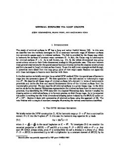
Similarly we define Gr , gR and gr . We will always assume 0 < r ≤ 1 ≤ R < ∞. It is easy to see that GR 7→ G, g R 7→ g(λ) = g R (Rλ), λ ∈ S 1 , is an isomorphism of groups. This way GR inherits naturally a Banach Lie group structure from G. The need for using two distinct circles is demonstrated clearly in Proposition 5.2 and Theorem 5.3.1 in [15]. Let p be a standard parabolic subalgebra of g and q its natural complement. By P and Q we denote the corresponding connected Banach Lie subgroups. Via (4.1.2) we thus obtain Banach Lie groups P R , P r , QR and Qr as well. For this paper the following Banach Lie groups are particularly important: (4.1.3)

H = GR × Gr ,

(4.1.4)

H− = QR × P r ,

(4.1.5)

H+ =

(

(g1 , g2 ) ∈ H : g1 ∈ GR and g2 ∈ Gr have the same holomorphic extension in the annulus

r < |z| < R

)

.

In particular, if r = R, then H+ is just the diagonal in H = G × G. The corresponding Lie algebras will be denoted by h, h− and h+ respectively. On Fig.1 below we indicate the regions of the complex plane z where the respective groups live.

21

R Q

H+

P

r

r

R

Fig.1 4.2

In what follows we will frequently use the facts listed below.

Theorem (4.2.1). H+ and H− are connected Banach Lie subgroups of H. Moreover, H− and H+ have the following properties: (a) H− H+ is open and dense in H. (b) H− H+ is analytically diffeomorphic with H− × H+ . (c) H+ and H− are closed in H. Proof. The first part of the theorem and Item (c) follow from Corollary (3.7.4) and the lemma below. To prove (a) and (b) we observe that h− + h+ = h and h− ∩ h+ = {0} holds [15]. From this it follows that the map

h− + h+ (h− , h+ )

→H 7→ exp h− exp h+

is a local diffeomorphism at 0; therefore H− H+ is open in H and, locally at the identity, analytically diffeomorphic with H− × H+ . −1 For general h− h+ ∈ H− H+ , consider a neighborhood U of h− h+ such that h−1 − U h+ can be mapped diffeomorphically into H− × H+ . From this, (b) follows, To see that H− H+ is dense in H, we pick an arbitrary g = (g R , g r ) ∈ H. Since QP is open and dense in G, in every neighborhood of g we can find a g˜ such that (˜ g r )−1 ∈ Qr P r . Hence we may assume that g r ∈ P r Qr . Write g r = pr q r . Then g = g R (µ), g r (λ) = g R (µ)q r (µ)−1 , pr (λ) q r (µ), q r (λ) . 22

If necessary, replace g R by gˆR arbitrarily close to g R such that gˆR (µ)q r (µ)−1 = qˆR (µ)ˆ pR (µ) ∈ P R P R . Then we obtain

gˆR (µ)q r (µ)−1 , pr (λ) = qˆR (µ)ˆ pR (µ), pr (λ) = qˆR (µ), pr (λ)ˆ pR (λ)−1 pˆR (µ), pˆr (λ) ,

where we used that P R naturally embeds in P r . Thus gˆR (µ), g r (λ) ∈ H− H+ and the proof is complete. Lemma (4.2.2).

H− ∩ H+ = {I}.

Proof. This is a coordinate dependent proof. We use the coordinates introduced earlier following §14.3 of [10]. Let (g1 , g2 ) ∈ H− ∩ H+ . Since g1 ∈ QR , the Laurent expansion of g1P (λ) about λ = 0 contains only nonpositive exponents. Therefore, there exists some P P n n h= P hn z n such that hn Rn λn = g1 ∈ Q and h r λ = g2 ∈ P . Since hn = 0 for n P n n n n ≥ 0, hn z converges for |z| ≥ r. Moreover, hn R λ ∈ P ∩ Q = {I}. Remark. The above section generalizes the setup in [15] to general loop groups as well as more general subgroups. §5. Factorization

5.1 In this section we recall some facts about the cyclic P element of g, all of which can be found in [10]. By the cyclic element we mean E := ei ∈ g, the sum of all canonical generators of canonical degree 1. Its centralizer, s := Centg E = Ker ad E = {F ∈ g : [E, F ] = 0}, is an abelian subalgebra of g, which is graded with respect to the canonical grading: (5.1.1)

s=

M

sk .

k∈Z

The integers k, for which sk 6= {0}, are called the exponents of g. If k is an exponent of g, then dimC sk is called the multiplicity of k. (1) It turns out that the multiplicity is always one, with the exception of D2m , m ≥ 2 [10, Ch.14]. Nevertheless the exponent 1 has always multiplicity one and the space s1 is spanned by E. (Remark 14.2 and table E0 in [10]). An important feature of E is that ad E : g → g is bijective on its image, or equivalently, (5.1.2)

g = Im ad E ⊕ Ker ad E .

An easy proof of this can be deduced by extending the argument given by Kac in [10, Prop. 14.2] for the case of g simple and finite dimensional. Finally, we remark that Im ad E is graded with respect to the canonical grading. 5.2 For every integer k we choose a nonzero element Ek ∈ sk , if possible, and let Ek = 0 otherwise. We will always assume E1 = E. Then (5.2.1)

{· · · , E−2 , E−1 , E0 , E1 , E2 , · · ·} 23

(1)

spans s in case g is not of type Dℓ , ℓ ≥ 4, ℓ even. In that case we choose two linearly inde′ pendent elements Eℓ−1 , Eℓ−1 . Note that 0 is never an exponent; thus E0 = 0. Nevertheless we include it for the sake of simplicity of notation. We set t := (· · · , t−2 , t−1 , t0 , t1 , t2 , · · ·)

(5.2.2) for tk ∈ R and k ∈ Z,

RZ = {t :

(5.2.3)

X

tk Ek ∈ g}.

k∈Z (1)

As above, we will double the coefficient ts if g is of type Dℓ multiplicity two. Define EkR ∈ gR as usual via EkR := Ek (µ) for

(5.2.4)

and the exponent s is of

µ ∈ SR,

Similarly we define Ekr ∈ gr . For this paper the following action of RZ on H will be of particular importance. (

(5.2.5)

(5.2.6)

t(h1 , h2 ) =

exp

RZ × H → H t, (h1 , h2 ) 7→ t(h1 , h2 ), X

k∈Z

tk EkR

!

h1 , exp

X

k∈Z

tk Ekr

!

h2

!

.

Note that EkR and h1 depend on µ ∈ S R , whereas Ekr and hr depend on λ ∈ S r . 5.3 We recall from Theorem(4.2.1) that H− H+ is open and dense in H. Therefore, if (h1 , h2 ) ∈ H− H+ , then also t(h1 , h2 ) ∈ H− H+ for all t in an open neighborhood of t = 0. The proof of the following Proposition is in immediate adaptation of that in [15, Proposition 3.6]. Proposition (5.3.1) If (h1 , h2 ) 6∈ H− H+ , then t(h1 , h2 ) ∈ H− H+ if t is contained in some open subset of {t; t1 6= 0}. So from now on we assume that (h1 , h2 ) ∈ H− H+ . Keeping this in mind we consider the Riemann-Hilbert splitting (5.3.1)

t(h1 , h2 ) = g − (t, µ)−1 , g + (t, λ)−1 bR (t, µ), br (t, λ) ,

such that the first factor lies in H− , the second one in H+ . Note that bR (t, µ) and br (t, λ) are analytic in t, since t(h1 , h2 ) is analytic and the map H− H+ → H− × H+ is an analytic diffeomorphism. ∂ Let ∂j denote ∂tj for any j ∈ Z. 24

Differentiating (5.3.1) and using that s is abelian, we get (5.3.2)

(5.3.3)

(5.3.4)

(5.3.5)

R (∂j bR )b−1 R = Ωj ,

where

− − −1 ΩR + g − EjR (g − )−1 j = (∂j g )(g )

r (∂j br )b−1 r = Ωj ,

and

where

Ωrj = (∂j g + )(g + )−1 + g + Ejr (g + )−1 .

We call Ωj the j th potential and call it positive (or negative) iff j > 0 (or j < 0). The equality of the mixed derivatives of bR , i.e. ∂ij bR = ∂ji bR , yields the equation (5.3.6)

R R R ∂ i ΩR j − ∂j Ωi = [Ωi , Ωj ],

(5.3.7)

∂i Ωrj − ∂j Ωri = [Ωri , Ωrj ].

The conditions (5.3.6) and (5.3.7) are usually called Zero-Curvature Conditions (ZCC). Recall from Proposition (2.2.2) that every p is defined by choosing a subset X of ˜ + . Let us simple roots which in turn defines a subset of the positive root system called △ ˜ + . Since △ ˜ + is finite, s is a finite, define s to be the maximal height of the roots in △ positive integer. We set s = 0 if X is empty. With this notation we can describe another important feature of the Ω∗j , ∗ = R or r: Proposition (5.3.2). (a) If j > 0, then there exists a Laurent polynomial Ωj in λ such that Ωj |S r = Ωrj and Ωj |S R = ΩR j . Moreover, Ωj ∈ p and Ωj contains only components of the p-degree between 0 and j, and the canonical degree between −s and j. (b) If j < 0, then there exists a polynomial Ωj in λ−1 such that Ωj |S r = Ωrj and Ωj |S R = ΩR j . Moreover, Ωj ∈ q and Ωj contains only components of the p-degree between j and −1, and the canonical degree between j − s and −1. Proof. (a) From (5.3.5) we see that Ωrj is in pr for r > 0. From (5.3.4) we know that Ωrj can be extended to the region between S r and S R . Now (5.3.3) and (5.3.2) show that only finitely many p-degrees (resp. canonical degrees) can occur in Ωrj . The rest is a matter of comparing Ωrj with ΩR j . For example, in order to count the canonical degrees we count R the powers of λ appearing simultaneously in Ωrj and ΩR j . For example, for j > 0, Ωj has degrees ≤ j whereas Ωrj has degrees ≥ −s on account of the first term in (5.3.5). All other cases are dealt with analogously.

25

§6. Systems of Partial Differential Equations obtained from Factorization 6.1 In this section we derive systems of PDE’s from the zero-curvature conditions (5.3.6) and (5.3.7). We treat here the case j > 0 for which we show that all potentials Ωj , j > 0, can be expressed in terms of a certain number of functions parametrizing Ω1 . We give an example of the generalized Drinfeld-Sokolov system generalizing the results of Drinfeld and Sokolov [3] for maximal parabolic subalgebras. We would like to add that the possibility of this extension is already mentioned in [3, p.2014] where it is referred to as the “partially modified” generalized KdV equations. In this chapter we will always assume (h1 , h2 ) ∈ H− H+ in the splitting equation (5.3.1). In view of Proposition (5.3.1) this is a very mild restriction. The assumption above implies that there exists some (cR , cr ) ∈ H+ such that (6.1.1)

h1 = h− cR

(6.1.2)

h2 = h+ cr

for some for some

h− ∈ QR h+ ∈ P r .

Then (5.3.1) shows (6.1.3)

g − (0, µ) = h− (µ) and g + (0, λ) = h+ (λ) .

Therefore, for sufficiently small t, there exist q(t, µ) ∈ qR

and p(t, λ) ∈ pr

such that (6.1.4)

(6.1.5)

g − (t, µ) = h− (µ) exp q(t, µ) , g + (t, λ) = h+ (λ) exp p(t, λ) .

Using this, the potentials defined in (5.3.3) and (5.3.5) can be expressed as (6.1.6)

− q −q ΩR + eq EjR e−q ) , j = Ad(h )((∂j e )e

and (6.1.7)

Ωrj = Ad(h+ )((∂j ep )e−p + ep Ejr e−p ),

r 6.2 As outlined above, we are trying to express all potentials ΩR j resp. Ωj , j > 0 in terms of a set of basic, “independent”, functions. To achieve this, we will make use of the following.

Lemma (6.2.1). (6.2.1)

Let h(t) ∈ g. Then (∂j eh )e−h =

X 1 (ad h)n−1 ∂j h . n!

n≥1

26

In other words, (∂j eh )e−h = ψ(ad h)∂j h, where ψ : C → C is the entire function defined by z e −1 z= 6 0 z , ψ(z) = 1, z=0 . Remark. For matrix groups, (6.2.1) can be proved by a straightforward induction. For a general proof, see [25, chapter II, Theorem 1.7] or [23, Ch.3, §6, Proposition 12]. Note that for any Lie group, (∂j eh )e−h is contained in its Lie algebra. In particular we have (6.2.2)

(∂j eq )e−q ∈ q

and

(∂j ep )e−p ∈ p .

6.3 In this section we will show how every positive potential Ωj can be expressed as a differential polynomial in the components of Ω1 . To accomplish this, we need the following: Lemma (6.3.1). For every sufficiently small q ∈ q there exist uniquely determined qI ∈ (Im ad E)− = (Im ad E) ∩ g−

and

qK ∈ (Ker ad E)− = (Ker ad E) ∩ g−

such that (6.3.1)

eq = eqI eqK

and qI + qK ∈ q. Proof. Recall (5.1.2): g = Im ad E ⊕ Ker ad E. canonically graded, we have g− = (Im ad E)− ⊕ (Ker ad E)−. On the other hand (Im ad E)− + (Ker ad E)− (6.3.2) (qI , qK )

Since Im ad E, and Ker ad E are q ⊂ g− , therefore the map → U− 7→ eqI eqK

is a local diffeomorphism. The last statement of the theorem is obtained by considering the curve etq and using the Baker-Hausdorff formula for small t. We are now ready to prove Theorem (6.3.2). For j > 0 the potential Ωj is a universal ∂1 -differential polynomial in Ω1 with rational coefficients. Remarks. By “y is a ∂k -differential polynomial in x” we shall mean that each component of y is a polynomial in the components of x and its derivatives with respect to x. The word “universal polynomial” means that the coefficients of the polynomial are independent of Ω1 . Proof. (a) We choose any h− ∈ Q such that g − (t) = h− exp(q) and exp(q) = exp(qI ) exp(qK ). We then substitute g − (t) = h− exp(q) into (6.1.4) and set j = 1 in (6.1.6) to get − qI −qI (6.3.3) ΩR + eqI (∂1 eqK )e−qK e−qI + eqI E R e−qI . 1 = Ad(h ) (∂1 e )e Since Ker ad E R is abelian, formula (6.2.1) shows (6.3.4)

(∂1 eqK )e−qK = ∂1 qK . 27

Using this and (6.1.7) we get (6.3.5)

qI −qI h− .ΩR + eqI (∂1 qK + E R )e−qI 1 = (∂1 e )e

−1 − R where h− .ΩR (h )ΩR 1 = Ad 1 , and where we have used that qK and E commute.

(b) We will show that qI and ∂1 qK are determined by h− .Ω1 . To see this, we rewrite (6.3.5) as (6.3.6)

qI (∂1 e−qI )eqI + e−qI h− .ΩR = ∂1 qK + E R . 1e

In the next step we compare terms of the same canonical degree. For qI , qK ∈ g− we may write: (6.3.7)

qI = qI,−1 + qI,−2 + . . . ,

(6.3.8)

qK = qK,−1 + qK,−2 + . . . .

Similarly, by Proposition (5.3.2), we have (6.3.9)

− R − R − R h− .ΩR 1 = (h .Ω1 )1 + (h .Ω1 )0 + (h .Ω1 )−1 + . . .

We will prove by induction on the canonical degree m that qI and ∂1 qK are determined by − R R h− .ΩR 1 . For m = 1 we obtain from (6.3.6) that (h .Ω1 )1 = E holds. For m = 0 we get [−qI,−1 , E R ] + (h− .ΩR 1 )0 = 0 R R Since (h− .ΩR 1 )1 = E and ad E is bijective on its image, qI,−1 is uniquely determined by h− .ΩR 1 . To illustrate the procedure we consider the case m = −1 separately. Here we have

1 qI,−1 , [qI,−1 , E R] 2 − R − [qI,−1 , (h− .ΩR ) ] + (h .Ω 1 0 1 )−1 = ∂1 qK,−1 .

− ∂1 qI,−1 + [−qI,−2 , E R ] +

The sum

[qI,−2 , E R ] + ∂1 qK,−1

− R is therefore some ∂1 -differential polynomial in (h− .ΩR 1 )0 and (h .Ω1 )−1 . By projecting R R on Im ad E along Ker ad E and vice versa, we conclude that each term in the sum is a − R ∂1 -differential polynomial in (h− .ΩR 1 )0 and (h .Ω1 )−1 . Thus ∂1 qK,−1 is a ∂1 -differential − R R polynomial in (h− .ΩR is bijective when restricted to its 1 )0 and (h .Ω1 )−1 . Since ad E − R image, qI,−2 is a ∂1 -differential polynomial in (h .Ω1 )0 and (h− .ΩR 1 )−1 . By the same token, for m ≤ −1, we obtain from (6.3.6) that

[qI,−i−1 , E R ] + ∂1 qK,−i 28

− R − R is some ∂1 -differential polynomial in (h− .ΩR 1 )0 , (h .Ω1 )−1 , · · · (h .Ω1 )−i , and by repeating the argument given for m = −1 we see that

qI,−i−1

and ∂1 qK,−i

are

− R − R ∂1 -differential polynomials in (h− .ΩR 1 )0 , (h .Ω1 )−1 , · · · (h .Ω1 )−i . From the definition of − h− .ΩR 1 we immediately see that we can separate off the explicit dependence on h . As a result of this operation qI,−i−1 and ∂1 qK,−i become R R ∂1 -differential polynomials in (ΩR and polynomials in the entries of h. 1 )0 , (Ω1 )−1 , · · · (Ω1 )−i − R Thus we can write qI,−i (h , Ω1 ) etc. (c) After these preparations we are able to prove the theorem. From Proposition (5.3.2) we know that for j > 0, Ωj has only components of nonnegative p-degree. Thus − qI (h ΩR j = (h )e

(6.3.10)

−

,ΩR 1 )

EjR e−qI (h

−

,ΩR 1 )

(h− )−1

(+)

,

since qK and EjR commute. Note that ΩR j is uniquely determined by qI , which in turn R R is uniquely determined by Ω1 . To see that ΩR j depends polynomially on Ω1 , we use the fact that g1 ⊕ g0 is a finite dimensional vector space and therefore any x ∈ g− , such that cdeg(x) is sufficiently negative, must be in q. Now, let us apply this remark to (6.3.10). We obtain that ΩR j

−

= (h )

N X i=0

(6.3.11)

−

= (h )

N X i=0

− −1 (+) R adi (qI (h− , ΩR 1 ))(Ej ) (h ) i

ad (

N X l=1

− −1 (+) R qI (h− , ΩR , 1 )−l )(Ej ) (h )

− R for sufficiently large N . Thus ΩR j depends on finitely many qI (h , Ω1 )−i , all of which − are differential polynomials in ΩR 1 and polynomials in the entries of h . However, by re− peating the whole argument for h in a neighborhood of the identity we conclude that R − qI (ΩR 1 ), ∂1 qK (Ω1 ), in other words, both are constants as functions of h . Since the dependence of qI,−i on h− is polynomial, thus analytic, we obtain that qI,−i is a differential − polynomial in ΩR 1 , with no explicit dependence on h . Moreover, we used only linear operations (projections, commutators) to determine qI , consequently, the coefficients in R qI (ΩR 1 )−i are all rational numbers independent of Ω1 . This completes the proof.

Below we will not use the superscripts R or r to distinguish the two circles appearing in our discussion. The context will clearly tell the reader if one needs to make a distinction. In particular we will not attach a superscript to E. Corollary (6.3.3). (6.3.12)

The ZCC ∂j Ωi − ∂i Ωj = [Ωj , Ωi ],

i, j > 0 ,

is a system of equations for the scalar components of Ω1 . In particular, for i = 1 we obtain a system of evolution equations for the scalar components of Ω1 . 29

We will discuss (6.3.12) for i = 1 in more detail later. There, it will be important to know a priori how many equations we expect to obtain. To this end we consider U = [q(−1) , E (1) ],

(6.3.13)

where the superscript denotes as usual the p-degree. We note that (h− E(h− )−1 )(1) = E (1) since h− ∈ Q. Thus, by (6.1.6), Ω1 −E ∈ U so essentially U is the space where ΩR 1 naturally lives. Proposition (6.3.4). Let q be any smooth function of t with values in q and set Ω1 = Ad(h− )((∂1 eq )e−q + eq Ee−q ) and Ωj = (Ad(h− eq )Ej )(+) , j > 0. Then ∂j Ω1 − ∂1 Ωj − [Ωj , Ω1 ] ∈ U .

Proof. note

We know that Ω1 − E and all its partial derivatives are contained in U. Next we ∂1 (Ad(h− eq )Ej ) = Ad(h− )([(∂1 eq )e−q , Ad(eq )Ej ]) = [Ω1 , Ad(h− eq )Ej ] .

Hence ∂j Ω1 − ∂1 Ωj − [Ωj , Ω1 ] = ∂j Ω1 − [Ω1 , Ad(h− eq )Ej ](+) + [Ω1 , Ωj ] (+) = ∂j Ω1 − Ω1 , Ωj + (Ad(h− eq )Ej )(−) + [Ω1 , Ωj ] (+) = ∂j Ω1 − Ω1 , (Ad(h− eq )Ej )(−) = ∂j Ω1 − E (1) , (Ad(h− eq )Ej )(−1) ∈ U, (1)

where we used that Ω1 = E (1) .

6.4 In the next section we intend to show that the entries of Ω1 , relative to a certain basis, are all ∂1 -polynomials in dim g0 “basic functions.” The present section collects all necessary algebraic facts needed in the proof of the forthcoming Theorem (6.5.1). The main idea of this theorem is to exploit (6.3.3) by projecting both sides of that equation onto a subspace of U given by the kernel of certain operator (Ker(B) in the notation f in the appearing in the proof of Theorem (6.5.1)). The dual of this subspace is W/W f that we study in notation of this section. It is exactly the relation between U, W and W this section. The discussion in this section deals exclusively with gf in . Therefore we omit the superscript “fin” in this section. First, we introduce the following notation. Let (.|.) denote the canonical nondegenerate symmetric bilinear form on g as in [10, Theorem 2.2]. We furthermore define (6.4.1)

b = g(0) ∩ (g− ⊕ g0 ) = b0 ⊕ b−1 ⊕ . . . ⊕ b−s , 30

where s is the maximal integer such that b−s 6= {0}. (6.4.2)

b∗ = g(0) ∩ (g0 ⊕ g+ ) = b0 ⊕ b1 ⊕ . . . ⊕ bs ,

(6.4.3)

U−k = [g−k−1 , E (1) ] , 0 ≤ k ≤ s

(6.4.4)

U = U0 ⊕ U−1 ⊕ . . . ⊕ U−s ,

(−1)

Wk = Ak ∈ gk : [q−k−1 , E]|Ak = 0 ,

(6.4.5)

W = W0 ⊕ W1 ⊕ . . . ⊕ Ws ,

(6.4.6)

fk = Ak ∈ Wk : (Ak |U−k ) = 0 , W

(6.4.7)

f=W f0 ⊕ . . . ⊕ W fs . W

(6.4.8) We also define (6.4.9a)

r−k := (Ker ad E) ∩ q−k

for

k = 1, . . . , s,

(6.4.9b)

rk := (Ker ad E) ∩ q∗−k

for

k = 1 . . . , s,

where q∗−k is the natural dual of q−k with respect to (.|.). Note that dim r−k = dim rk for k = 1, . . . , s. f We collect some information about the dimensions of the vector spaces U, W and W. P P ∨ We will use the following notation. For α ∈ △, α = ki α αi we set ht(α) = ki . More ∨ generally, for a fixed X ⊂ Π we set pht(αi ) = 0 if i ∈ Π, 1 otherwise. Theorem (6.4.1). (a)

(b)

Wk = Ak ∈ gk : [E, Ak ] ∈ bk+1 for k = 0, . . . , s . dim W = dim b − dim g0 +

s X

dim r−k

s X

dim rk .

k=1

(c)

f = dim b + dim U + dim W 31

k=1

Proof.

(a) We know that Wk = Ak ∈ gk : q−k−1 [E, Ak ] = 0 = Ak ∈ gk : [E, Ak ] ∈ g(0) ∩ gk+1 = bk+1 .

The latter equality holds because, for 1 ≤ k ≤ s, (q−k )⊥ ∩ gk = g(0) ∩ gk . Indeed, if xα ∈ q−k )⊥ ∩gk then the height of α , ht(α), equals k. On the other hand the corresponding pht(α), when only roots from X are counted, satisfies pht(α) ≥ 0. We want to show that pht(α) = 0. Assume therefore that pht(α) > 0. Then pht(−α) < 0 and x−α ∈ q−k . Since (x−α , xα ) 6= 0 we get a contradiction as xα ∈ (q−k )⊥ . This proves that pht(α) = 0. For k = s + 1, on the other hand, q⊥ −(s+1) ∩ gs+1 = 0 ≡ bs+1 . (b) Since (.|.) is nondegenerate on g−k × gk , we get from (6.4.5) the relation dim Wk = dim gk − dim[q−k−1 , E] . Furthermore (6.4.10)

dim Wk = dim gk − dim q−k−1 + dim r−k−1

for k = 0, 1, . . . , s − 1 .

For Ws we note that q−s−1 = g−s−1 , thus: Ws = As ∈ gs : [g−s−1 , E] | As = 0 (6.4.11) = (Ker ad E)s . From (6.4.10) and (6.4.11) , we get dim W = dim g0 +

s−1 X

(dim g−k − dim q−k ) − dim q−s

k=1

+ dim(Ker ad E)s +

s X

dim r−k .

k=1

Since g−k = q−k ⊕ b−k , dim b−k = dim g−k − dim q−k , k = 1 . . . s. Therefore ! s s X X dim W = dim g0 + dim b−k − dim g−s − dim(Ker ad E)s + dim r−k . k=1

k=1

Since dim g0 = dim b0 , we obtain that (6.4.12)

s X dim W = dim b − dim gs − dim(Ker ad E)s + dim r−k . k=1

By virtue of [10, Proposition 14.3a], (6.4.13)

dim gs − dim(Ker ad E)s = dim g0 , 32

thus (6.4.14)

dim W = dim b − dim g0 +

s X

dim r−k .

k=1 (0)

(c) Let Vk = (U−k )⊥ ∩ bk . Then the space Vk ⊂ gk satisfies for k = 0, 1 . . . , s Vk ⊆ bk , dim U−k + dim Vk = dim bk (U−k | Vk ) = 0, .

(6.4.15)

and

fk = Vk ⊕ rk holds. We claim that W fk , we decompose E = E (0) + E (1) and derive from the definitions To verify Vk ⊂ W of Vk and Uk immediately that [Vk , E (1) ] = 0

(6.4.16)

(0)

Moreover, since E (0) ∈ g1 , we have (6.4.17)

[Vk , E (0) ] ⊂ bk+1 .

This implies (6.4.18)

[Vk , E] ⊂ bk+1 .

From (a) we now obtain Vk ⊂ Wk . This together with the definition of Vk and (6.4.8) shows (6.4.19)

fk . Vk ⊂ W

fk . Since Vk ⊂ g(0) and rk ∈ g(+) , we have Vk + rk = Since rk ⊥ p we obtain that rk ⊆ W Vk ⊕ rk . fk . Note that Now let Ak ∈ W (6.4.20)

bk ⊕ (q−k )∗ = gk .

Let Bk ∈ bk , Ck ∈ (q−k )∗ ⊆ g(+) such that Ak = Bk + Ck . Then (6.4.21)

(Ak | U−k ) = (Bk | U−k ) + (Ck | U−k ) .

Here the second term vanishes, since Ck ∈ g(+) and U−k ∈ g(0) . Therefore, also Bk ∈ Vk , fk by (6.4.8), and in fk by (6.4.19). This in turn means that Ck ∈ W whence Bk ∈ W particular Ck ∈ Wk . Hence, by virtue of (a), (6.4.22)

[Ck , E] ∈ bk+1 . 33

Since Ck ∈ g(1) and E = E (0) + E (1) , [Ck , E] ∈ bk+1 ∩ g(+) = {0} .

(6.4.23) Thus

Ck ∈ (Ker ad E) ∩ (q−k )∗ ,

(6.4.24)

f k ⊆ Vk + rk . whence W f k = Vk ⊕ rk . This proves that W Now we have (6.4.25)

Hence (6.4.15) implies

fk = dim Vk + dim rk dim W

fk = dim U−k + dim Vk + dim rk dim U−k + dim W = dim bk + dim rk

(6.4.26)

Summation over k = 0, . . . , s completes the proof.

6.5. In this section we will roughly show that among the scalar components of Ω1 , a subset of cardinality rank g = dim g0 can be chosen, such that the remaining functions are ∂1 -differential polynomials in those. More precisely, we show Theorem (6.5.1).

There exists a basis c1 , . . . , cm of U, such that in the expansion Ω1 = E

(1)

+

m X

uk ck

k=1

the coefficient functions ul+1 , . . . , um are ∂1 -differential polynomials in u1 , . . . , uℓ , where ℓ = rank g = dim g0 . Proof. (6.5.1)

From Proposition (5.3.2) we know that (0)

(1)

Ω1 = Ω1 + Ω1

,

where the superscript denotes as usual the p-grading. From (6.1.6) we obtain (6.5.2)

(1)

(1)

Ω1 = E 1

and we write Ω1 = E + U0 + . . . + U−s , where U−k is homogeneous of canonical degree −k. Next we write (6.3.3) in the form (6.5.3) Ω1 = Ad(h− ) (∂1 eqI )e−qI + eqI (∂1 qK + E)e−qI . Decomposition into components of canonical degree −j yields:

(6.5.4a)

U0 = [qI,−1 , E] + R0 (h− ), 34

− where R0 (h− ) = [h− −1 , E] for some h−1 ∈ g,

U−j = [qI,−(j+1) , E]+∂1 qK,−j

+Rj qI,−1 , . . . , qI,−j , qK,−1 , . . . , qK,−(j−1) , h− ,

(6.5.4b)

1 ≤ j ≤ s,

where Rj is a differential polynomial in its arguments. From Theorem A.1.2, it follows that all dependence on qK in (6.5.4b) drops out, thus (6.5.4b) simplifies to (6.5.4c) U−j = qI,−(j+1) , E + Rj (qI,−1 , . . . , qI,−j , h− ) .

We can, furthermore, simplify (6.5.4c) by eliminating qI,−1 , . . . qI,−j . Indeed, using (6.5.4a) and solving (6.5.4c) for qI,−k , 0 ≤ k ≤ j, we can write (6.5.4c) as: (6.5.5)

˜ j (U0 , . . . , U−j+1 , h− ), U−j = qI,−(j+1) , E + R

1≤j≤s.

˜ j is independent of h− . Since R ˜j Note, however, that in the neighborhood of the identity, R − ˜ ˜ is analytic in h we get that Rj = Rj (U0 , . . . , U−j+1 ). Relation (6.5.5) cut out a subset S of U ⊗ R, where R is the germ of holomorphic maps at x = 0. We proceed now to describe fj . S. We apply (·|Aj ) to (6.5.5), where Aj ∈ Wj /W By (6.4.6), (6.4.8) and (6.5.4a) we get ˜ −j (U0 , . . . , U−j+1 )|Aj , 0 ≤ j ≤ s . (6.5.6) (U−j |Aj ) = R fj relations for the components of (Ω1 )−j = U−j . Let us now Thus we get dim Wj − dim W choose a basis b1 , . . . , bm of U, which is consistent with the canonical grading, i.e. X X X U0 = uj bj , U−1 = uj bj , . . . , U−s = uj b j 0 0. (c)

Ωh−1 = Ωk−1 if f R

R

gh− = gk− e−t−1 E−1 m− et−1 E−1

(7.3.3)

, m− ∈ QR

and (7.3.4)

gh+ = gk+ γ + , γ + ∈ Γr ∩ P r

and

∂−1 γ + = ∂−1 m− = 0 .

(d) If Ωh−1 = Ωk−1 then Ωhj = Ωkj for all j < 0. (e) If Ωh1 = Ωk1 and Ωh−1 = Ωk−1 then Ωhj = Ωkj for all j ∈ Z. (f ) If Ωh−1 = Ωk−1 then Ωh1 = Ωk1 (g) If Ωh−1 = Ωk−1 then Ωhj = Ωkj for all j ∈ Z. (h) If Ωh−1 = Ωk−1 and Ωh1 = Ωk1 then gh− = gk− γ − and gh+ = gk+ γ + with γ + and γ − independent of t1 and t−1 . Proof. (a) From §5.3 we know (7.3.5)

(Ωh1 )R = (∂1 gk− )(gh− )−1 + gh− E R (gh− )−1 R

R

= ∂1 (gh− et1 E )(gh− et1 E )−1 , (7.3.6)

r

r

(Ωh1 )r = ∂1 (gh+ et1 E )(gh+ et1 E )−1 .

It is straightforward to show that (7.3.7)

(∂j g)g −1 = (∂j g˜)˜ g −1 if and only if g = g˜gˆ and ∂j gˆ = 0 . 44

Thus: R

R

r

r

(7.3.8)

gh− = gk− et1 E γ − e−t1 E

(7.3.9)

gh+ = gk+ et1 E m+ e−t1 E

for some γ − ∈ GR , m+ ∈ Gr independent of t1 . Setting t1 = 0 shows γ − ∈ QR and m+ ∈ P r . Moreover, R

R

(gk− )−1 gh− = et1 E γ − e−t1 E ∈ QR ,

(7.3.10)

thus γ − ∈ Γr by Theorem (3.7.2). This settles the “only if” part. The “if” part is straightforward. (7.3.11)

R

R

(Ωh1 )R = ∂1 (gk− γ − et1 E )(gk− γ − et1 E )−1 = ∂1 gk− (gk− )−1 + gk− (∂1 γ − )(γ − )−1 (gk− )−1 + gk− γ − E R (γ − )−1 (gk− )−1 = (Ωk1 )R , since ∂1 γ = 0 and [γ − , E R ] = 0 .

(7.3.12)

r

r

(Ωh1 )r = ∂1 (gkr et1 E m+ )(gk+ et1 E m+ )−1 = (∂1 gk+ )(gk+ )−1 + gk+ E r (gk+ )−1 = (Ωk1 )r ,

since ∂1 m+ = 0. (b) Again, from 5.3 and (a) we know (7.3.13)

R

R

(Ωhj )R = ∂j (gh− etj Ej )(gh− etj Ej )−1 R

R

= ∂j (gk− γ − etj Ej )(gk− γ − etj Ej )−1 , = (Ωkj )R + gk− (∂j γ − )(γ − )−1 (gk− )−1 This shows (7.3.14)

(Ωhj )R − (Ωkj )R ∈ qR

On the other hand, we know from Proposition (5.3.1) that (Ω∗j )R ∈ pR , for j > 0. Whence (Ωhj )R − (Ωkj )R ∈ pR . This shows (Ωhj )R = (Ωkj )R . Note that the latter condition defines Ωj uniquely, since two Laurent polynomials that coincide on the circle are equal. Thus: Ωhj = Ωkj . (c) As in (a) one concludes (7.3.15)

R

R

gh− = gk− et−1 E−1 m− e−t−1 E−1 45

r

r

gh+ = gk+ et−1 E−1 γ + e−t−1 E−1

(7.3.16)

for some m− ∈ QR , γ + ∈ P r , such that ∂−1 γ + = ∂−1 m− = 0. Moreover, r

r

(gk+ )−1 gh+ = et−1 E−1 γ + e−t−1 E−1 ∈ P r ,

(7.3.17)

thus γ + ∈ Γr ∩ P r by Theorem (3.7.3). This settles the “only if” part. The “if” part is straightforward. (d) As in (b) one computes r

r

(Ωhj )r = ∂j (gh+ etj Ej )(gh+ etj Ej )−1

(7.3.18)

r

r

= ∂j (gk+ γ + etj Ej )(gh+ γ + etj Ej )−1 = (Ωkj )r + gk+ (∂j γ + )(γ + )−1 (gk+ )−1 . This shows (Ωhj )r − (Ωkj )r ∈ pr .

(7.3.19)

On the other hand we see from (5.3.3) that R (0) ΩR ∈ qR , j − (Ej )

(7.3.20) thus

(Ωhj )R − (Ωkj )R ∈ qR .

(7.3.21) This shows that Ωhj = Ωkj . (e) follows from (b) and (d) (f) Using (c) we derive (7.3.22)

r

r

(Ωh1 )r = ∂1 (gh+ et1 E )(gh+ et1 E )−1 r

r

= ∂1 (gk+ γ + et1 E )(gk+ γ + et1 E )−1 = (Ωk1 )r + gk+ (∂1 γ + )(γ +)−1 (gk+ )−1 . We need to show that the second term vanishes. From (5.3.3) and (7.3.13) we know that (7.3.23)

(0)

R R ΩR 1 − E ∈ (g− ⊕ g0 )

thus (7.3.24)

(0)

(Ωh1 )r − (Ωk1 )r = Ad(gk+)((∂1 γ + )(γ + )−1 ) ∈ (g− + g0 )r .

Now (∂1 γ + )(γ +)−1 ∈ (Ker ad E ∩ p)r . At this point we apply Theorem (B.1.2) from the Appendix B stating that Ker ad E ∩ (0) g = 0. Thus min pdeg(Ad(gk+)((∂1 γ + )(γ + )−1 ) ≥ 1 which implies the claim. 46

(g) obvious from (b), (d), (f), (h) follows from (a) and (c). Remark. The results of Theorems (7.1.1) and (7.3.1) give the following picture (where “−→” means “determines uniquely”): Ω1

−→

Ωj (j > 0)

−→

Ωj (j < 0)

ր ↑

a ց

Ω−1 Proposition 7.3.2. Proof.

If Ker ad E ∩ g(−1) = {0}, then Ωh1 = Ωk1 implies Ωh−1 = Ωk−1 .

Assume Ωh1 = Ωk1 . Then by Lemma (7.2.1) we have ∂1 Ωh−1 = ∂1 Ωk−1 , hence Ωh−1 = Ωk−1 + C−1 ,

(7.3.8)

where C−1 depends on t−1 only. (We ignore variables different from t1 and t−1 here.) By Proposition (7.3.1 a) (7.3.9)

gh− = gk− γ − (t−1 )

and γ − (t−1 ) ∈ Γ− ∩ Q .

This implies (setting gh− (0, 0) = (h− )−1 , gk− (0, 0) = (k − )−1 − ) γ − (0) = k − (h− )−1 ∈ Γ− .

(7.3.10)

Next we evaluate the (−1) - potentials, using the formulas of §5.3: R (Ωh−1 )R = (∂−1 gk− )(gk−)−1 + gk− (∂−1 γ − )(γ − )−1 (gk− )−1 + gk− E−1 (gk− )−1

= (Ωk−1 )R + gk− (∂−1 γ − )(γ − )−1 (gk− )−1 From (7.3.8) we conclude (∂−1 γ − )(γ − )−1 = (gk− )−1 C−1 gk− .

(7.3.11) From (7.1.6) we see that (7.3.12)

C−1 ∈ q(−1) .

Upon decomposing C−1 with respect to the canonical grading we get (7.3.13)

C−1 = c−1 + · · · + c−m ,

for some finite m.

Let (7.3.14)

(gk− )−1 = k − exp(r−1 + r−2 + · · ·), 47

where k − ∈ Q is t and x independent. Thus (7.3.11) turns into (7.3.15) (∂−1 γ − )(γ − )−1 = k − exp ad(r−1 + r−2 + s) C−1 (k − )−1 . Let

(∂−1 γ − )(γ − )−1 = s−1 + s−2 + · · · .

(7.3.16)

Now compare in (7.3.15) and (7.3.16) components of the same canonical degree. Note that k − ∈ Q). First, we consider cdeg = −1 : we obtain s−1 . Now (7.3.12) and (7.3.9) imply s−1 = c−1 ∈ Ker ad E ∩ g(−1) = {0}, thus s−1 = c−1 = 0. Next, we consider cdeg = −2 : Since s−1 = 0 and c−1 = 0, we obtain s−2 = c−2 . As above we conclude s−2 = c−2 = 0. The remainder of the proof goes by induction on the canonical degree, thus yielding C = 0. To see that the condition of the previous Proposition is nontrivial we briefly discuss the following two examples: Example 1: In the case of minimal parabolics the p-grading coincides with the canonical grading. Thus the condition Ker ad E ∩ q−1 = {0} does not hold and Ω−1 is not uniquely determined by Ω1 . To see that one only needs to examine (7.1.14) and (7.1.15). However, one has a natural parametrization of Ω1 in terms of w ∈ g0 , namely Ω1 = E + ∂1 w, which gives Ω−1 = ew E−1 e−w . It remains an interesting open question whether one can find a natural parametrization in terms of elements of g0 in each case Ker ad E ∩ q(−1) 6= {0}. (1) Example 2: Let gf in be of type A3 , and g = sℓ4 (Aw ) where Aw is the Wiener Algebra w.r.t. some weight w (cf. 1.1). Denote by Eij the 4 × 4-matrix with 1 in the (i, j)-position and 0’s elsewhere. A set of Chevalley generators is given by e0 = λE41 , e1 = E12 , e2 = E23 , e3 = E34 , f0 = λ−1 E14 , f1 = E21 , f2 = E32 , f3 = E43 , hi := [ei , fi ]

for

i = 0, 1, 2, 3.

Let p be the standard parabolic subalgebra generated by g0 ⊕ g+ , f1 and f3 , i.e. P n   P n  λ An λ Bn   n≥0 n≥0   P P : An , Dn ∈ sl2 (C), Bn , Cn ∈ gl2 (C) . p= λn Cn λn Dn   n≥0

n≥0

It is easy to see that

q

(−1)

=

0 B

λ−1 A 0

48

: A, B ∈ gl2 (C)

.

Thus, q(−1) ∩ Ker ad E 6= {0}, since E−2 = E

−2

=

0 I2

λ−1 I2 0

∈ q(−1) ∩ Ker ad E ,

where I denotes the 2 × 2 identity matrix. (1) For “nontwisted”g, i.e. g of type Xℓ we are able to determine all the cases where the condition of Proposition 7.3.2. is violated, i.e. where Ker ad E ∩ g(−1) 6= {0} . The result is as follows [27]. ◦

(1)

◦

Theorem (7.3.3). Let g be of type Xℓ , and h the Coxeter number of g , where g is finite dimensional and simple of type Xℓ . Let k be a positive exponent of g. The following are equivalent: (a) k divides h (b) There is a parabolic subalgebra p of g such that (Ker ad E)−k ∩ g(−1) 6= {0} .

Remark The relations between h, k and p for which (Ker ad E)−k ∩ g−1 6= 0 have been investigated in detail in [27]. The following table summarizes the main result of that paper. Xℓ ℓ

Bℓ Cℓ Dℓ E6 E7 E8 F4 G2

h ℓ+1 2ℓ 2ℓ 2ℓ − 2 12 18 30 12 6

exponents k 1, 2, · · · , ℓ 1, 3, · · · , 2ℓ − 1 1, 3, · · · 2ℓ − 1 1, 3, · · · , 2ℓ − 3, ℓ − 1 1, 4, 5, 7, 8, 11 1, 5, 7, 9, 11, 13, 17 1, 7, 11, 13, 17, 19, 23, 29 1, 5, 7, 11 1, 5

k|h? depends on depends on depends on depends on k=4 k=9 none none none

ℓ ℓ ℓ ℓ

This shows in particular that the situation is fairly easy for the exceptional Lie algebras. We will not pursue this any further in this paper.

49

7.4 We present below an example of a “negative potential” and the associated differential equation. We use the following notation: the derivatives with respect to x and t are denoted either by ∂x,t or by using x or t as a subscript. We will follow the procedure described in the last two chapters. The most important point we would like to emphasize is that by results of Section 6 it suffices to work in the neighborhood of the identity of the group G. This allows one to carry out computations on a Lie algebraic level. In this example, we want to closely investigate to which extent Ω1 determines the quantities involved in the splitting procedure. We consider the case of (1) A1 . Let gf in = sℓ2 (Aw ) where Aw is the Wiener Algebra w.r.t. some weight w (cf. 1.1). Denote by Eij the 2 × 2-matrix with 1 in the (i, j)-position and 0’s elsewhere. A set of Chevalley generators is given by e0 = λE21 , e1 = E12 , f0 = λ−1 E12 , f1 = E21 , α∨ i := [ei , fi ] for

i = 0, 1.

Let p be the standard parabolic subalgebra generated by g0 ⊕ g+ , f1 , i.e. P n  P n   λ an λ bn   n≥0 n≥0   P P p= : an , bn , cn ∈ C . λn cn − λn an   n≥0

n≥0

The p-grading in this case agrees with the grading according to the powers of λ, i.e. pdeg(Eij λk ) = k. To further simplify the computation we observe that by Theorem (6.3.2) we can use the formula (7.4.1)

qI −qI ΩR + eqI (∂j qK + EjR )e−qI . j = (∂j e )e

In fact we can ignore the size of the contour and set R = 1. Our goal is to compute Ω−1 . To this end we will have to find the relevant contributions from both qI and qK . We first decompose these two with respect to the canonical grading. This for the case at hand amounts to setting c-deg(Eij λk ) = j − i + 2k. This makes E homogeneous of degree 1, consequently Ej has degree j. We write qI = qI,−1 + qI,−2 + . . . , similarly

qK = qK,−1 + qK,−2 + . . . .

By (7.1.6) the essential part of Ω−1 lives in g(−1) . In the present case this gives (7.4.2)

(−1)

g

−1

=λ

a c

b −a

,

a, b, c ∈ C.

We observe that the minimal canonical degree appearing in Ω−1 is −3. We will therefore use the following variables {qI,−i , qK,−i , i = 1..3}. In fact qK,−2 = 0 as E −2 6∈ g. Furthermore, it is useful to observe that v ∈ Im ad(E) ∩ gi if and only if there exists a diagonal matrix a = diag(α, −α), α ∈ C, such that v = aE i . A similar result for ker ad(E) states that a has 50

to be a multiple of the identity. Thus we can parametrize {qI,−1 , qI,−2 qI,−3 , qK,−1 , qK,−3 } in terms of 5 scalars {h1 , h2 , h3 , w1 , w3 } by forming the appropriate diagonal matrices. Using (7.1.6) we can now express Ω−1 in terms of these variables. This is a purely Lie algebraic computation and the result is:

(7.4.3)

Ω−1 =

2h1 +∂t h2 +2∂t w1 h1 λ

(1 − ∂t h1 + ∂t w1 ) + a

1+∂t h1 +∂t w1 λ − 2h1 +∂t h2λ+2∂t w1 h1

where a = −λ−1 (2h21 + h1 ∂t h2 − h2 ∂t h1 + 2∂t w1 h21 + 2∂t w1 h2 + 2h2 − ∂t w3 + ∂t h3 ). We parametrize the potential Ω1 as follows u (7.4.4) Ω1 = λ + ux − u2

1 −u

.

Now we use (7.4.1) to express {h1 , h2 , h3 } in terms of u and its x derivatives. The result is : (7.4.5)

h1 =

1 1 1 1 1 1 u, h2 = − ux + u2 , h3 = uxx − uux + u3 . 2 2 4 4 2 12

From the proof of Theorem (6.3.2) we know that ∂x qK is a differential polynomial in Ω1 , in the case of the present example we obtain: (7.4.6)

w1,x =

1 ux , 2

1 1 1 w3,x = − (ux )2 − u2 ux + uuxx . 4 8 4

We would like to point out that in fact w1 is uniquely determined. This is clear from the fact that if exp(qI ) exp(qK ) and exp(qI ) exp(qK ) exp(cE−1 ) satisfy (7.4.1) and both are in Q then this implies exp(cE−1 ) ∈ Q for some c ∈ C. Note, however, that in the present f in example g(−1) ∩ ker ad(E) = 0, in particular E−1 6∈ q. Moreover the group Q = Q has the property that Q − I consists of functions analytic around ∞ in λ and being zero there. This implies w1 = 12 u. Substituting (7.4.5) and w1 back into Ω−1 yields: Ω−1 =

−

ux,t −2uut −2u 2λ

1+b

1+ut λ ux,t −2uut −2u 2λ

where

1 b = −λ−1 (−8ux + 8u2 + 7u2 ut + 2uxxt − 6ux ut − 6uuxt − 8w3,t ). 8 In the next step we use the ZCC to express ∂t w3 in terms of ∂x − ∂t derivatives of u. The ZCC reads: (7.4.7)

∂t Ω1 − ∂x Ω−1 + [Ω1 , Ω−1 ] = 0.

The final formula for Ω−1 takes now a simple form: 51

(7.4.8)

Ω−1 =

t −2u − uxt −2uu 2λ

1−

1+ut λ uxt −2uut −2u 2λ

−4ux +2u2 +2u2 ut +uxxt −4ux ut −2uuxt 2λ

.

What now remains to do is to use the latter form of Ω−1 to compute the ZCC. A straightforward computation leads to a simple ZCC: 1 λ

0 uxxxt − 4uxx − 8uxt ut − 4ut uxx

0 0

= 0.

Summarizing, the Ω−1 and Ω1 - generated flows give rise to the following partial differential equation: (7.4.9)

uxxxt = 4uxx + 8uxt ut + 4ut uxx .

With the help of the simple substitution z(x, t) = u(4x, t) + t we can reduce this equation to (7.4.10)

zxxxt = zxx zt + 2zx zxt .

We would like to add that from the point of view of the KdV theory, to which one passes by setting u = zx , equation (7.4.10) is an integro-differential equation. Thus, if one thinks of it as a member of the KdV hierarchy, then one is confronted with the question of its utility for the KdV theory. This point remains to be clarified. Another remark is in order here. Equation (7.4.10) is a special case of the Bogoyavlenskii equation [1], namely, (7.4.11)

zxv = zxxxt − zxx zt − 2zx zxt ,

where v is the third independent variable.The factorization problem for this equation was formulated in [21]. Equation (7.4.10) is one of many reductions of (7.4.11), namely the one corresponding to the symmetry generator ∂v (z is v independent). Another reduction which has been studied is the one corresponding to the symmetry generator ∂t −∂v . The resulting equation was studied by Hirota and Satsuma [2] as a model for shallow water waves. In particular the aforementioned authors found its soliton solutions. We would like to conclude the discussion of this section with the remark that, since the time the first draft of this paper was written, a theory of ‘negative‘ potentials has been further advanced by G. Haak [29].

52

Appendix A: Proofs of Propositions (3.3.1) and (3.5.2) Proposition (3.3.1). Let P = PX be a parabolic subgroup of G and w ∈ W . Then ◦ ◦ ◦ + + ∼ (a) P = PX = G X Q+ X = QX G X = G X × QX . w w w (b) The stabilizer U− in U− of wP ∈ G/P is U− = U− ∩wP w−1 . Moreover, dim U− < ∞. w (c) There exists a closed subgroup V− of U− such that group multiplication induces a w diffeomorphism U− ∼ × V−w . = U− Proof. (a) First we note that g(0) and g(+) are closed complementary subalgebras of p. Let G(0) and G(+) denote the corresponding integral subgroups of P . Arguing with the gradings as before, we see Ad (G(0) ∩ G(+) ) = {I}. But this implies G(0) ∩ G(+) = {I} as in the proof of Theorem 2.4.1. Therefore P = PX = G(0) G(+) ∼ = G(0) × G(+) by Corollary 3.1.4. ◦ ◦ ◦ + + (0) ∼ ∼ G G = Q To prove P = PX = G X Q+ = = X X × QX it now suffices to show G X X ◦

G X × AQ , where AQ = H ∩ Q+ X . We want to apply Corollary (3.1.4). To this end we ◦ note that g and aQ are closed complementary subalgebras of g(0) . Therefore, it suffices to ◦ prove G X ∩ AQ = {I}. In view of the Iwasawa decomposition [11, §5] of G ∼ = K × A × U+ ◦ ◦ ◦ ◦ ∼ and G X = KX × A × (G X )+ we see that it suffices to show AQ ∩ A = {I}. We know that ◦

◦

◦

◦

[g X , aQ ] = 0, so Ad AQ |G X = I. Therefore for g ∈ AQ ∩ A we have Ad g|G X = I. Since ◦ ◦ g ∈ A ∈ G X , g = I follows. w < ∞ it suffices to note (b) The first statement is easy to verify. To see that dim U− l(w) = #{α ∈ △+ ; w(α) < 0}. (c) The following proof is an adaptation of [12;8.6]. Set uw− = u − ∩ wpw−1 . In the overlaying Kac-Moody algebra we see that uw − is invariant under the action of the w Cartan algebra. Therefore u − is a direct sum of root spaces. Moreover, v w− = u − ∩ wpopp w−1 , popp being the opposite parabolic, is a closed subalgebra of u − such that u − = uw− ⊕ v w− . We note that popp can be obtained by applying the Chevalley involution ω of g to p [10;§1.3]. Therefore, by [23, Ch.3, §6, Theorem 2], there exists a connected subgroup V−w of U− with Lie algebra vw− . More precisely, we have the following closed, connected subgroups w U− = U− ∩ w P w−1

and

V−w = U− ∩ w P opp w−1 (k)

with Lie algebra uw− and v w− respectively. Let u− denote all elements in u − of (k) sufficient high degree ≥ k. Then u − ⊂ v w− and uw− is contained in the natural (k) ˆ− = u− modu(k) complement of u − in u − . Moreover, uk− is an ideal in u− , whence u − ˆw is a finite dimensional, nilpotent, Lie algebra, with complementary subalgebras u − and ˆw ˆw ˆw vˆw − . It is not difficult to see that for the corresponding groups U− , U+ and V− we have ˆ− = U ˆ w Vˆ w . Hence U− = U w V w and the multiplication map m : U w × V w → U− U − − − − − − is surjective. It is well known that m is everywhere regular. Therefore it suffices w now to show that m is injective. This is equivalent with U− ∩ V−w = {I}. Let w ˆ w ∩ Vˆ w . Since U ˆ− is finite dimensional we know g ∈ U− ∩V−w . Then we map g to gˆ ∈ U − − w w ˆ− has a faithful representation gˆ = exp(ˆ u) = exp(ˆ v), u ∈ u− , v ∈ v − . Moreover, u (k) consisting of nilpotent matrices. Hence u ˆ = vˆ; i.e. u = v + q, q ∈ u− . But this (k) implies u = 0, whence g ∈ U− . Since we can choose k arbitrary large, g = I follows. 53

Proposition (3.5.2).

For every w ∈ W/WX we have CX (w) =

[

CX (w′ )

M

where M = {w′ ∈ W/WX , w′ w}. Proof.

At first we follow [24]. Let w′ be X-reduced and w′ w. Then for some i w′ = w1 ri w2 , where w1 (αi ) > 0 and w2−1 (αi ) > 0 and w = w1 w2 .

Then

B− w1 w2 P = B− (w1 U−αi w1−1 )w1 w2 (w2−1 Uαi w2 )P = B− w1 U−αi Hi Uαi w2 P .

We know that the closure of U−αi Hi Uαi , where Hi = exp Chi , is a subgroup Gi of G which is isomorphic with SL(2, C). In particular, ri ∈ Gi , whence B− w′ P = B− w1 ri w2 P ⊂ B− w1 U−αi Hi Uα w2 P ⊂ B− w1 U−αi Hi Uα w2 P = B− w1 w2 P . S This proves CX (w′ ) ⊂ CX (w). Conversely, CX (w) = w′ ∈J CX (w′ ), where J is some subset of the set W ′ of X-reduced elements. Assume first that X = ∅, i.e. B = PX . Then we consider the representation of π of g in glres described in [12;Ch.6]. Our assumptions on the weights w imply that π is continuous. In particular, π(C∅ ) ⊂ π(C∅ ). From [12,Proposition (7.3.3)] we can now conclude (see also [12, chap.8, in particular Theorem (8.7.2)]) that w′ w for all w′ ∈ J. Consider now the general case. We note that [ CX (w) = C∅ (ww). ˜ w∈W ˜ X

S It is important to note that here WX is finite. Therefore, CX (w) = w∈W C∅ (ww). ˜ This ˜ X implies [ [ [ CX (w) = C∅ (w′ ) = CX (w′ ). w′ w X−reduced

′ w∈W ˜ ˜ X w w w

54

Appendix B: Injectivity Problems In the following we prove two theorems concerning the map ad E and its restriction to g . (0)

Lemma B.1.1.

Ker ad E = Ker ad E−1 for any E−1 ∈ (Ker ad E)−1 \{0}.

Proof. Using the Chevalley involution ω, we get that ω(Ker ad E) ⊂ Ker ad E−1 . Moreover, by Proposition 14.3 a in [10] we get that ω(Ker ad E) = Ker ad E. So Ker ad E ⊂ Ker ad E−1 . By the same argument we get Ker ad E−1 ⊂ Ker ad E. Theorem B.1.2. Let g be an affine Kac-Moody algebra and p 6= g a standard parabolic subalgebra of g. Then: Ker ad E ∩ g(0) = {0}. Proof.

The proof is broken down into nine subclaims:

Claim 1 : Ker ad E ∩ g0 = {0} . Indeed the integer 0 is never an exponent [6; §14]. Claim 2 : Ker ad E ∩ g(0) ⊆ Ker ad E (0) ∩ g(0) . Let S ∈ g(0) such that [S, E] = 0. Since E = E (0) + E (1) , [S, E (0)] + [S, E (1) ] = 0. The first term is in g(0) , whereas the second in g(0) , thus [S, E (0) ] = 0. Claim 3 : The map

ad E (0) : g(0) → g(0)

is nilpotent.

Clear, since cdeg E (0) = 1 and g(0) is finite dimensional. Claim 4 : There are elements F (0) , H (0) ∈ g(0) such that Q : = CF (0) C ⊕ H (0) ⊕ CE (0) is isomorphic to sl(2, C), i.e. H (0) = [E (0) , F (0) ], [H (0) , E (0) ] = 2E (0) , [H (0) , F (0) ] = −2F (0) . Since adE (0) is nilpotent, this follows from the Theorem of Jacobson-Morozov. Here, however, we can define the elements F (0) and H (0) explicitly. Let X X X F (0) : = ci fi , then H (0) = ci [ei fi ] = ci hi , X X [H (0) , E (0)] = ci [hi , ej ] = ci aij ej ! X X X ci aij fj , cj and [H (0) , F (0) ] = ci cj [hi , fj ] = − j

i

˜(0) := [g(0) , g(0) ] , the semisimple part of g(0) . where (aij ) =: A is the Cartan matrix of , g (0) Since ˜g is finite dimensional, A is an invertible matrix, whence the system of equations ! X X X 2ej (ci aij ) ej = j

j

i

has a unique solution. It is easy to verify that this gives F (0) and H (0) as required. Claim 5 : α(H (0) ) = 2(ht α) for every root α of g(0) . This statement is a direct consequence of [H (0) , ei ] = 2ei , [H (0) , fi ] = −2f i. 55

(0)

Claim 6 : Ker ad E (0) ∩ g− = {0} . Since g(0) is an a-module, by Weyl’s Theorem it is the direct sum of a finite number of irreducible a-modules: g(0) = V1 ⊕ · · · ⊕ Vr . Consider one of these irreducible a-module V = Vs . Since a ∼ = sℓ(2, C), there is a basis of V consisting of eigenvectors of ad H (0) : v−m , v−m+2 , · · · , vm−2 , vm such that [H (0) , vj ] = j·vj . From (5) we see that m is always an even number, thus dim V is odd. Since also [E (0) , vj ] = vj+2 , the kernel of ad E (0) in V is spanned by the highest-weight vector vm . Since, by (5), (0) this vector has a nonnegative canonical degree we conclude that Ker ad E (0) ∩ g− = {0} . (0)

Claim 7 : Ker ad E ∩ g− = {0} . This is a direct consequence of (2) and (6). (0)

Claim 8 : Ker ad E−1 ∩ g+ = {0} . Copy the proof of (7), interchanging ei and fi . (0)

Claim 9 : Ker ad E ∩ g+ = {0} . This claim follows from (8) and Lemma 6.4.1. Altogether, (1), (7) and (9) yield the claim.

56

References 1. Bogoyavlenskii, O.I., Breaking solitons in 2+1 - dimensional integrable equations, Russian Math. Surveys 45, (1990), no.4, 1-86. 2. Hirota, R., Satsuma, J., N-soliton solutions of Model Equations for Shallow Water Waves, J.Phys.Soc.Japan 40, (1976), 611 3. Drinfel’d, V.G.,and Sokolov,V.V., Lie algebras and equations of Korteweg-deVries type, Journal of Soviet Mathematics, 30, (1985), 1975-2036. 4. Wilson, G., The modified Lax and two-dimensional Toda lattice equations associated with simple Lie algebras, Ergodic Theory and Dynamical Systems, 1, (1981), 361-380. 5. Sato M., Soliton equations as dynamical systems on infinite dimensional Grassmann manifolds, RIMS Kokyuroku 439, (1981), 30-46 6. Segal, G., Wilson, G., Loop groups and equations of KdV type, Publ.Math. I.H.E.S. 63, (1984), 1-95 7. Garland, H., The arithmetic theory of loop groups, Publ.Math. I.H.E.S. 52, (1980), 5-136. 8. Peterson, D.H., Kac, V.G., Infinite flag varieties and conjugacy theorems, Proc. Natl. Acad. Sci. USA 80, (1983), 1778-1782. 9. Tits, J., Resumé de cours, Collège de France, Paris, (1981) 10. Kac, V., Infinite dimensional Lie algebras, Cambridge University Press, (1985). 11. Goodman, R., Wallach, N. R., Structure and unitary cocycle representations of loop groups and the group of diffeomorphisms of the circle, J.Reine Angew. Math., 347, (1984), 69-133. 12. Pressley, A.,Segal, G.,Loop groups and their representations, Oxford University Press, (1986). 13. Dorfmeister, J., Szmigielski, J., Riemann-Hilbert Factorizations and Inverse Scattering for the AKNS-Equations with L1 -Potentials I, Publ. RIMS, Kyoto University 29, (1993), 911-958. 14. Szmigielski, J., Infinite dimensional manifolds with translational symmetry and nonlinear partial differential equations, Ph.D Dissertation, University of Georgia-Athens, GA, (1987). 15. Dorfmeister, J., Wu, H., Constant mean curvature surfaces and loop groups, J.reine angew. Math. 440, (1993), 43-76. 16 Dorfmeister, J., Haak, G., On symmetries of constant mean curvature surfaces, Part II: Symmetries in a Weierstrass type representation, to appear 17 Dorfmeister, J., Haak, G., On constant mean curvature surfaces with periodic metric, to appear in Pacific J.Math. 18. Szmigielski, J., On the soliton content of the self dual Yang-Mills equations, Phys.Lett.A 183, (1993), 293-300. 19. Dorfmeister, J., Banach Manifolds of Solutions to Nonlinear Partial Differential Equations, and Relations with Finite-Dimensional Manifolds, Proceedings of Symposia in Pure Mathematics 54, (1993), 121-139. 57

20 de Groot, M.F., Hollowood, T.J., and Miramontes, J.L., Generalized Drinfeld-Sokolov hierarchies Comm. Math. Phys. 145, (1992), no.1, 57-84. 21 Burroughs, N.J., de Groot, M.F., Hollowood, T.J., and Miramontes, J.L., Generalized Drinfeld-Sokolov hierarchies. II. The Hamiltonian structures, Comm. Math. Phys. 153, (1993), no.1, 187-215. 22 Fehèr, L., Harnad, J., and Marshall, I., Generalized Drinfeld-Sokolov reductions and KdV type hierarchies, Comm. Math. Phys. 154, (1993), no.1, 181-214. 23. Bourbaki, B., Groupes et algèbres de Lie. Ch. 1, Hermann, Paris, 1964; Ch. 2, et 3, Hermann, Paris, 1972; Ch.4,5 and 6, Hermann, Paris, 1968; Ch. 7 et 8, Hermann, Paris, 1975; Ch. 9, Masson, Paris, (1982). 24. Kac, V.G., Peterson, D. K., Regular functions on certain infinite-dimensional groups, in Arithmetic and Geometry, Progress in Math. 36, 141-166, Birkhäuser, Boston, (1983). 25. Helgason, S., Differential geometry, Lie groups and symmetric spaces. Academic Press, New York, (1978). 26. Beals, R., Deift, P., Tomei, C., Direct and Inverse Scattering on the Line. Amer.Math. Soc.., Providence, RI, (1992). 27. Gradl, H., A result on exponents of finite-dimensional simple Lie algebras and its application to Kac-Moody algebras, Linear Algebra Appl 233, (1996), 189-206. 28. Sattinger, D.H., Szmigielski, J., Factorization and the dressing method for the GelfandDikii hierarchy, Physica D 64, (1993), 1-34. 29. Haak, G., Negative flows of the potential KP-hierarchy, Trans. Amer. Math. Soc. 348, (1996), no.1, 375-390.

58

Systems of PDEs obtained from factorization in loop groups

Systems of PDEs obtained from factorization in loop groups

Suggest Documents

FACTORIZATION SYSTEMS FOR SYMMETRIC CAT-GROUPS ...

Determination of silanol end groups in polysiloxanes obtained from ...

Factorization properties of paratopological groups

Loop groups, Clusters, Dimers and Integrable systems

Factorization of unitary representations of adele groups

Factorization and Entanglement in Quantum Systems

Hamiltonian PDEs - FroM-PDE - Sissa

An XML representation of DAE systems obtained from continuous-time ...

Collaborative Factorization for Recommender Systems

A factorization theorem for topological abelian groups

MINIMAL SURFACES VIA LOOP GROUPS

Loop groups and noncommutative geometry

UTILIZATION OF DIGESTATE OBTAINED FROM

montmorillonite nanocomposites obtained from

Factorization in categories of systems of linear partial differential

REAL LOCI OF BASED LOOP GROUPS

Phylogeny of Pneumocystis Obtained Obtained From ... - Lume - UFRGS

fourier analysis of multigrid methods for general systems of pdes

Theory of ground state factorization in quantum cooperative systems

Travelling wave solutions of nonlinear systems of PDEs by ... - UEM

Compatibility, multi-brackets and integrability of systems of PDEs

be obtained from fluorescence depolarization in

The Order Completion Method for Systems of Nonlinear PDEs Revisited

The Order Completion Method for Systems of Nonlinear PDEs ...