Task types, link functions & probabilistic modeling in experimental pragmatics∗ Michael Franke Seminar für Sprachwissenschaft Eberhard Karls Universität Tübingen Abstract Recent years have seen increased interest in experimental approaches in pragmatics, but pragmatics has not been an experimental discipline from the start. As a result, a common problem is one of mapping between theory and experimental data: how do established theoretical notions carry over to precise predictions about to-be-expected data?; conversely, what exactly do particular experimental tasks measure, expressed in notions meaningful to pragmatic theory? I argue here that explicit probabilistic modeling can provide a key for tackling these fundamental issues.
Keywords: probabilistic pragmatics, link functions, regression models, truth-value judgement task, rating scale task
1
Towards theory-based statistical modeling
Experimental pragmatics is a relatively young scientific enterprise, but it builds on long traditions in especially theoretical linguistics, psycholinguistics and experimental psychology. Its developmental lineage is both virtue and vice: on the one hand, experimental pragmatics can tap into rich theoretical and methodological knowledge bases, but, on the other hand, it may unduly hamper itself by a suboptimal combination of elements from its theoretical and experimental ancestors. I argue here that experimental pragmatics can benefit from endorsing the richness of formal cognitive modeling, thereby going beyond mere hypothesis testing and out-of-the-box regression analyses, techniques which I will call “theory-free.” The alternative is to spell out, in the same data-generating model, both: (i) a theoretical component (inspired by pragmatic theory), and (ii) a link function (inspired by ∗ Dorothea
Knopp helped with designing the experiments, and processing the data. Fabian Dablander assisted in implementing the experiments. Their help is much appreciated. I am also grateful to Judith Degen and Bob van Tiel for sharing data and thoughts. This work was supported by the Institutional Strategy of the University of Tübingen (Deutsche Forschungsgemeinschaft, ZUK 63) and the Priority Program XPrag.de (DFG Schwerpunktprogramm 1727).
1
variant task type fillers many & most no. participants in analysis
Table 1
A
B
C
D
ordinal present 119
ordinal absent 114
binary present 109
binary absent 107
Experimental variants
standard statistical modeling) that describes how the theoretical predictions map onto observable choice probabilities in a given task. For concreteness of example, Section 2 introduces what superficially looks like inconclusive evidence obtained from two different task types: while a truth-value judgement (TVJ) task indicates no contextual interference effects, a rating-scale judgement (RSJ) task does. Discrepancies between results from different tasks are relatively common in the recent literature, often leading to deadlocks and inability to reach a consensus about important theoretical issues (e.g., the methodological debate about whether there are “embedded implicatures” (c.f. Geurts & Pouscoulous 2009, Chemla & Spector 2011, Geurts & van Tiel 2013)). The probabilistic model of Section 3 is able to resolve this apparent tension. Putative differences between task types are accommodated by suitable link functions, so that it is possible to maintain a uniform and explicit picture of what exactly is measured in either task and how experimental manipulations relate to theoretical notions of interest. 2
Case study: typicality of quantifiers
van Tiel (2014) and Degen & Tanenhaus (2015) independently looked at typicality ratings for scalar some in sentences like “Some of the circles are black” in combination with different pictures of varying numbers of black and white circles. These studies used a rating scale task and showed that the typicality of some is a gradient function of the number of black circles (see left of Fig. 1). The data for this paper comes from a partial replication of these studies with two additional manipulations: (i) the task type and (ii) the presence/absence of quantifiers many and most as additional fillers in the experiment. Participants were recruited via Mechanical Turk and assigned to one out of four variants in a between-subjects design (see Table 1). On each trial of any variant, subjects were presented with a randomly generated picture of 10 circles, some of which white, the others black. In variants A and B, subjects rated whether a sentence was a good description of a picture on a 7-point rating scale. In variants C and D,
2
ordinal
binary
1.00
● ●
means
0.75
● ●
● ●
●
● ●
●
●
●
●
alternatives
● ●
0.50
●
●
alt. present alt. absent
● ●
0.25
●
●
●
0.00
●
0.0
2.5
5.0
7.5
10.0 0.0
2.5
5.0
7.5
10.0
condition (no. black balls)
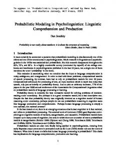
Figure 1
Means of ordinal 7-point rating scale data (left), with the ith degree coded as i−1 6 , and means of binary truth value judgements with true judgement coded as 1.
subjects judged whether a sentence was true of the given picture or not. Participants rated 13 sentences in variants A and C, which contained fillers with many and most, and 8 in variants B and D, which did not contain these fillers. Each sentence was either a random control sentence, a critical sentence with some, or a filler sentence with many or most (for variants A and C only). Sentences were presented in pseudorandom order with some constraints, the most important of which was that in variants A and C, exactly one filler with many and one with most preceded the first encounter of a critical some sentence. Mean responses from between 107 and 119 participants per variant (see Table 1) are shown in Fig 1. Does presence or absence of fillers with many or most have an effect on the data under either task type? Visual inspection suggests that presence of alternatives many and most seems to be reflected in ordinal RSJs, but perhaps not in binary TVJs. Statistical analyses in support of this conclusion exists. Analyses that suggest otherwise do too. The issue to debate is not which statistical analysis is least careless or most adequate and certainly not which one is correct. There are more general questions. What do TVJs and RSJs measure? Same thing or different? Is whatever is measured influenced by the presence or absence of alternatives? If so, how? Is what is measured influenced by experimental manipulations in the same way in either task? What does it even mean to measure something with a task, and, most importantly, how is whatever we measure related to a rich body of pragmatic theory? It is difficult, if not impossible, to address this by testing null-hypotheses or calculating regression models. But that does not mean that statistical modeling is at its end, of course. The key is to inject pragmatic theory.
3
3
A probabilistic model
The (simplified) structure of (Bayesian) regression modeling is this: (1)
predictor value + link function = likelihood of data .
For each data point d we compute a predictor value xd as a (e.g., linear) function of a vector of coefficients ~b, that represents the influence of all relevant explanatory factors, and the values for these factors associated with d. The predictor value xd is then mapped onto a likelihood P(d | ~b, . . . ) by a link function suitable for the task. Standard regression models are, in a manner of speaking, theory-free. The predictor value xd is retrieved from some general-purpose, mathematically convenient function of coefficients ~β. In contrast, a theoretically informed data-generating model would mold domain-specific assumptions into a specific, tailor-made map from factors to predictor value xd . Unlike in theory-free models, the latent predictor variable xd can be conceptually meaningful in theory-driven models. From the point of view of a theoretically informed model, xd is what a task measures. Link functions can remain the same for theory-free and theory-inspired models. To ask whether two tasks could plausible measure the same thing, is to find a plausible theoretical model for xd , plug it into different link functions, and see whether data from both tasks can be handled in the combined model. Let’s do that. Pragmatic model of the predictor value. We need a measure for the pragmatic felicity of statement “Some of the circles are black” in each of the 11 conditions (0, 1, . . . 10 of the 10 circles being black). Pragmatic felicity is influenced by, among other things, the purpose of the conversation and, being a relative notion, the pragmatic felicity of other possible expressions. Inspired by game theoretic and probabilistic pragmatics, the assumption here is that pragmatic felicity is the (scaled) expected utility of the some statement, relative to that of alternative statements, to a speaker who describes a given picture for a literally interpreting listener (because such a speaker demonstrably implements Gricean language use). Fix conditions c ∈ {0, 10} for the number of black balls and messages m ∈ M = {none, one, two, three, some, many, most, all}, where some is taken to mean “at least one,” most to mean “more than half” and many to mean “at least 4” (fixed ex post by subjects’ actual judgements of many-sentences). Degrees of salience of alternatives to some are estimated from the observed data (see Franke 2014). A literal listener interprets message m as a random state in which m is true. If c is the actual state and the literal listener guesses c0 , then the speaker’s utility is a parameterized function of the distance between c and c0 (Nosofsky 1986): (1)
U(c, c0 ; π) = exp(−π (c − c0 )2 ) . 4
Here, π is a free parameter for pragmatic precision: if π → ∞ only guessing the true state has positive utility; as π decreases near guesses have more and more utility; for π = 0 all interpretations are equally good. A speaker’s expected utility of using message m in condition c is: X (2) EU(m, c ; π) = PLL (c0 | m) U(c, c0 ; π) , c0
where PLL (c | m) is the probability that the literal listener chooses interpretation c for m. To reflect competition between alternative expressions, as Gricean pragmatics would have us do, consider the scaled expected utility for some in each condition, relative to any set X ⊆ M of entertained alternatives (this always contains some): (3)
EU∗ (c, X ; π) =
EU(some, c) − minm∈X EU(m, c) . maxm∈X EU(m, c) − minm∈X EU(m, c)
Speakers may not entertain a fixed set of alternatives X. If the probability of entertaining alternatives is given by a probability vector ~s of length 7, and if we assume (crudely) that probabilities of entertaining alternatives are all independent, Q Q the probability that set X is entertained is P(X | ~s) = m∈X sm m∈M\X (1 − sm ). The central tendency of relative pragmatic felicity of some in condition c is then: X (4) F(c ; ~s, π) = P(X | ~s) EU∗ (c, X ; π) . X
This is a theory-driven predictor for TVJs and RSJs alike. Link functions. Let’s consider standard link functions from regression modeling for our task types. For binary response variables, like from TVJs, the link function is usually given by a logistic function whose output is fed into a binomial distribution. If the data is a number k of true responses out of n observations, then the likelihood is Binomial(k, n, p) with probability p = (1 + exp(−γ(x − θ)))−1 given by a logistic function of predictor value x with threshold θ and gain γ. For ordinal response variables, like from RSJs, xd is fed into a thresholded probit model and the outcome is piped into a multinomial distribution. Let ~k be a vector of counts with kd the number of choices of degree d ∈ 1, . . . 7 on the 7-point rating scale, and n the number of observations. Then the likelihood is Multinomial(~k, n, ~p) where ~p is a probability vector of length 7, calculated as follows. Each degree d is associated with an interval Id , the boundaries of (some of) which are free model parameters. Intervalls for all degrees form a partition of the reals. We assume that, on each choice occasion, the predictor value x is perturbed by Gaussian noise with standard deviation σ. The degree corresponding to the interval in which 5
messages i ∈ {1, . . . , 7} s−i
s+i
si+/− ∼ Beta(1, 1) 1 π
π
∼ Gamma(0.5, 0.5)
Fc+/− = F(c ; ~s +/− , π) σ ∼ Uniform(0, 0.4)
Fc−
Fc+
δd∈{1,...,6} ∼ Normal(d/7, 14) δ0 = −∞; δ7 = ∞ θ, γ
δcd , σ
θ ∼ Normal(0.5, 0.2) 1 γ
A pcd
A kcd
B pcd
B kcd
pCc
pcD A/B pcd =
kCc
kcD
∼ Gamma(1, 1)
R δcd
δcd −1
Normal(x, Fc+/− , σ) dx
pC/D = (1 + exp(−γ(Fc+/− − θ)))−1 c A/B A/B A/B kcd ∼ Multinomial(pcd , nc )
ncA
ncB degrees d ∈ {1, . . . , 7}
Figure 2
nCc
ncD
C/D kC/D ∼ Binomial(pC/D c c , nc )
condition c ∈ {0, . . . , 10}
Probabilistic graphical model (see Lee & Wagenmakers 2015).
the perturbed value resides is chosen. Hence, the probability pd of observing a choice of degree d on the rating scale is the probability that the Gaussian perturbation of x lies in Id . A formalization of this idea is contained in Figure 2. Data-driven inference. Figure 2 gives the full probabilistic model, using the conventions for probabilistic graphical models of Lee & Wagenmakers (2015). Arrows indicate dependencies of variables. The observed data, in shaded boxes, informs the values of the latent parameters. Latent parameters without dependencies are constrained by suitable prior distributions, as given on the right in Figure 2. The most important detail is that two vectors of salience of alternative messages are used, ~s + for the case where alternatives are present, and ~s − otherwise. Estimates of the joint posterior over latent parameters, conditional on the data, were obtained by MCMC sampling using JAGS (Plummer 2003). After a burn-in of
6
10,000 samples, every second of another 10,000 samples entered into the analysis. Convergence was assessed by visual inspection and Rˆ values (Gelman & Rubin 1992). Posterior predictive checks confirm that the model, when using posteriors of model parameters, generates virtual data that is indistinguishable from the actual. In this weak sense, the model seems to “work” alright: it is possible to think that the same underlying value generated both TVJs and RSJs at the same time. The most interesting inference is that of posteriors of salience of messages. Figure 3 shows estimates from the MCMC samples. Model and data suggest that most is made more salient by its presence, but not many. Empirical and theoretical consequences of this prediction remain to be explored. 4
Conclusions
Pragmatic notions of theoretical interest can be crafted into quantitative models of latent predictor values. Combined with standard link functions from regression modeling, we obtain theory-driven, data-generating models, with the help of which we can start to make sense of otherwise eluding pieces of data. The particular model given in this paper is merely an example. It raises many further issues. These issues, however, are meaningful to experimental pragmatics and could not be perceived clearly and discussed stringently without any concrete model on the table. It is an empirical question whether this model, or any other is the right way to think about truth-value or rating scale judgements. To decide between competing models, statistical model comparison based on suitable data is necessary. Doing so will give a better understanding of what different tasks are measuring, how a measure is influenced by factors of relevance and what we may or may not conclude from experimental data. In sum, experimental pragmatics will benefit from explicit, theory-driven probabilistic modeling of the whole data-generating process. References Chemla, Emmanuel & Benjamin Spector. 2011. Experimental evidence for embedded scalar implicatures. Journal of Semantics 28. 359–400. http://dx.doi.org/10. 1093/jos/ffq023. Degen, Judith & Michael K. Tanenhaus. 2015. Processing scalar implicatures: A constraint-based approach. Cognitive Science 39. 667–710. http://dx.doi.org/10. 1111/cogs.12171. Franke, Michael. 2014. Typical use of quantifiers: A probabilistic speaker model. In Paul Bello, Marcello Guarini, Marjorie McShane & Brian Scassellati (eds.), Proceedings of cogsci, 487–492. Austin, TX: Cognitive Science Society.
7
salience (posterior estimate)
1.00 ●
●
0.75
●
●
●
0.50 ●
0.25
●
alternatives ●
absent
●
present
●
● ● ●
●
● ●
0.00 none
one
two
three
many
most
all
message
Figure 3
Estimates of posteriors of ~s + and ~s − . Bars are 95 % highest density intervals (i.e., an interval of values with non-negligible posterior credence levels), dots are posterior means.
Gelman, Andrew & Donald B. Rubin. 1992. Inference from iterative simulation using multiple sequences (with discussion). Statistical Science 7. 457–472. Geurts, Bart & Nausicaa Pouscoulous. 2009. Embedded implicatures?!? Semantics & Pragmatics 2(4). 1–34. http://dx.doi.org/doi:10.3765/sp.2.4. Geurts, Bart & Bob van Tiel. 2013. Embedded scalars. Semantics & Pragmatics 6(9). 1–37. http://dx.doi.org/10.3765/sp.6.9. Lee, Michael D. & Eric-Jan Wagenmakers. 2015. Bayesian cognitive modeling: A practical course. Cambridge, MA: Cambridge University Press. Nosofsky, Robert M. 1986. Attention, similarity, and the identification-categorization relationship. Journal of Experimental Psychology: General 115(1). 39–57. Plummer, Martyn. 2003. JAGS: A program for analysis of Bayesian graphical models using Gibbs sampling. In Kurt Hornik, Friedrich Leisch & Achim Zeileis (eds.), Proceedings of the 3rd international workshop on distributed statistical computing, . van Tiel, Bob. 2014. Quantity matters: Implicatures, typicality, and truth: Radboud Universiteit Nijmegen dissertation.
Michael Franke Wilhelmstraße 19 72076 Tübingen
[email protected]
8