Feb 24, 2012 - University of Minnesota ... Minneapolis, MN 55455-0159 USA .... lies in the guard's unbounded 2D wedge (whose apex angle is free to be set) ...
Sensor Placement and Selection for Bearing Sensors with Bounded Uncertainty
Technical Report
Department of Computer Science and Engineering University of Minnesota 4-192 Keller Hall 200 Union Street SE Minneapolis, MN 55455-0159 USA
TR 12-006 Sensor Placement and Selection for Bearing Sensors with Bounded Uncertainty Pratap Tokekar and Volkan Isler
February 24, 2012
Sensor Placement and Selection for Bearing Sensors with Bounded Uncertainty (Extended Abstract)
Pratap Tokekar and Volkan Isler∗
Abstract We study the problem of placing sensors so as to accurately estimate the location of a target in a given environment. We focus on bearing sensors (such as cameras, microphone arrays) which are commonly used for target localization. We seek to discover and exploit the geometric structure associated with both the sensing model and the estimation process in order to obtain sensor placement schemes with performance guarantees. We use a geometric model to represent the sensing uncertainty: Each measurement yields an unbounded 2D wedge with angular width 2α around the measurement (α is an input parameter representing the maximum sensing noise). The wedge is guaranteed to contain the true location of the target. The target is localized by intersecting the wedges obtained from all sensors. The quality of the placement is given by the area or diameter of the intersection in the worst-case (i.e. regardless of the target’s location). We study the bi-criteria optimization problem of placing a small number of sensors while guaranteeing a worst-case bound on the estimation error. ∗ Our main result is a constant-factor approximation for this problem: Let UD and UA ∗ be the ∗ diameter and area uncertainty achieved by an optimal algorithm using n sensors. We show ∗ that at most 9n∗ sensors placed on a triangular grid has diameter uncertainty of at most 5.88UD π π ∗ and area uncertainty of at most 7.76UA , when the sensing noise 0 < 2α ≤ 2 . For 2 < 2α < π, we bound the number sensors sufficient to have a bounded target estimate. When the maximum sensing noise 2α ≥ π, we show that there always exists a set of measurements, for any placement of n sensors, such that the intersection of all wedges is unbounded. In obtaining these results, we provide some interesting structural properties which may be of independent interest. First, we study general placements and obtain a lower bound on the best uncertainty that can be achieved when placing n sensors on the plane. We then focus on the grid-based placement scheme and show that a placement of n sensors placed on a triangular grid does not deviate much from this lower-bound. This latter result also yields a sensor selection mechanism: We show that in the triangular grid, only a constant number of sensors need to be activated to achieve the upper-bound.
∗
The authors are with the Department of Computer Science and Engineering, University of Minnesota, Minneapolis, MN, USA. {tokekar,isler}@cs.umn.edu
1. Introduction Sensor placement for target localization is a fundamental problem in robotics and sensor networks. The goal is to place sensors so as to accurately estimate the unknown location of a target in a given environment. A good sensor placement scheme can improve the performance of a sensor network in applications such as detecting an intruder in surveillance, robot navigation using exteroceptive measurements, and providing location information to mobile devices for location-aware computing. Most sensors employed for localization have a strong structure associated with their sensing and measurement model. This structure plays a critical role in how information from multiple sensors can be combined. In this paper, we study the sensor placement problem for bearing sensors. Bearing sensors are commonly used in robotic and networked sensor systems: Monocular cameras, microphone/acoustic arrays, directional radio antennas, passive infrared receivers, etc. all measure bearing towards a target. We consider the scenario when the output of each sensor is a bearing corrupted with unknown but bounded noise. Bounded noise models provide a useful alternative to probabilistic models especially when a precise device model is not available (perhaps due to the difficulty of calibration or changing device parameters). In the bounded uncertainty model, the true bearing to the target is guaranteed to lie in a 2D wedge which is centered at the measured bearing and has an apex angle equal to the maximum sensing noise. Measurements from multiple sensors are combined by intersecting the corresponding sensing wedges. The intersection yields an estimate for the target’s location. The uncertainty in the estimate is usually taken to be the diameter or the area of the intersection. We seek worst-case quality guarantees for our estimate: Given the true location of the target, imagine an adversary choosing the noise values for sensors. The true location can be anywhere in the intersection and we would like this set to be “small” no matter where the target is.
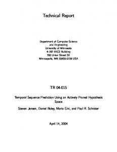
Figure 1: An example of the target estimate obtained by combining sensing wedges from all sensors π π , 15 and π5 . The true target is marked (marked as circles) when the maximum sensing noise is 25 by a cross. We consider a simple workspace for the problem: The target can lie anywhere within a square without any obstacles or visibility constraints. Even in this basic setting, devising a sensor placement scheme is tricky. It is intuitively clear that the optimal placement should be some kind of a uniform grid. However it is not clear if the grid should be square, triangular or some other shape. Further, optimizing parameters of the grid (e.g. resolution) is not straightforward because as illustrated in Figure 1, the estimate is obtained by combining measurements from all sensors. This
2
makes it difficult to express its area or diameter in closed-form in order to optimize grid parameters. Our contributions: We study the bi-criteria problem of minimizing the number of sensors and finding a placement in the workspace to guarantee a desired level of worst case uncertainty. First, we relate the worst-case uncertainty of a placement to the radius of the largest empty circle in the workspace (Lemma 2). Based on this relationship, we present lower bounds on the number of sensors required to achieve a desired uncertainty (Corollary 1 & Corollary 2). Next, we study simple sensor configurations and bound the maximum uncertainty when the target lies inside an equilateral triangle or regular hexagon with sensors placed on the vertices, as a function of the side length (Lemma 3 & Lemma 4). We then use these results to study the performance of a triangular placement (Lemma 6). This analysis provides a natural placement scheme with constantfactor approximation guarantees for placing sensors. Specifically, in a square workspace, when the maximum sensing noise is less than π4 we get a constant-factor approximation (Theorem 1). For sensing noise between π4 and π2 , we bound the number of sensors sufficient to ensure bounded intersection of sensing wedges (Lemma 5). When the maximum sensing noise is greater than π2 , we show there always exists a set of measurements for any placement of n sensors with an unbounded intersection of sensing wedges (Lemma 1). Therefore, in this last case, no placement can guarantee bounded error. In obtaining these results, we also show that one can obtain good estimates by activating only a constant number of sensors (Corollary 3). This result is important for sensornetwork applications with energy or bandwidth constraints. We start with an overview of related work.
2. Related Work The problem of optimizing the placement of sensor nodes in sensor networks research has been well studied [8]. A large amount of research has focused on self-localization of stationary sensor networks. For example, Agarwal et al. [1] studied the problems of localization, clustering and sensor suspension by refining the self-localization of a network of sensors with noisy but bounded uncertainty and correlated measurements of some environmental characteristic. In our present work, we assume that the locations of the sensors themselves are accurately known and focus on the complementary problem of placing sensors so as to localize targets. The Art Gallery Problem [6] is a classical problem of placing the minimum number of guards (or sensors like omnidirectional cameras), usually in polygonal environments, such that a target present anywhere within the polygon is visible from at least one guard. The original version of the problem only considers detection (or seeing) the target with a single guard. There is no notion of localizing the target, which could require combining measurements from multiple guards. Recently, Eppstein et al. [3] introduced a variant of placing a minimum number of “angle guards” in a polygon, to decide whether a target lies in the interior of the polygon. Each angle guard detects if a target lies in the guard’s unbounded 2D wedge (whose apex angle is free to be set) without any visibility constraints. The target location is said to be in the interior of the polygon if and only if the location lies in the intersection of wedges from two or more guards whose intersection is known to lie in the interior of the polygon. The paper presents bounds on the number of guards for various classes of polygons, as well as a 2-approximation for the general case. While this sensing model considers uncertainty in the sense that the measurement is a wedge, there is no notion of measurement noise or quality of localization (the goal is to decide if the target is inside or not). In this paper, we
3
specifically consider the uncertainty due to bounded noise in bearing sensors. The uncertainty in the target estimate obtained by combining bearing measurements depends on the relative position of the sensors and the target. For example, if the sensors are nearly collinear with the target, the resulting estimate will have significant uncertainty. With this as motivation, Efrat et al. [2] studied the following two variants of the Art Gallery Problem: minimize the number of guards such that (i) each point in the polygon is visible from at least two sensors with relative angle between them constrained to a desired interval, or (ii) each point is visible from at least three sensors enclosing the point. For both problems, the authors presented a log factor approximation, up to a fine discretization parameter. In addition to the relative angles, the uncertainty in estimation is also affected by the distance of the target from the sensors. The Geometric Dilution of Precision (GDOP) is one such measure giving in closed form, the relation of uncertainty with distance to target and relative angles. Tekdas and Isler [7] studied the problem of placing a minimum number of bearing sensors using GDOP as the objective function. They presented a placement scheme which guarantees that for any target location there are always two sensors whose GDOP is a constant factor of the GDOP achieved by two sensors from an optimal placement. In our work, we do not restrict the estimation process to use only two sensors. Instead, we compare our performance against an optimal placement combining measurements from possibly all sensors. Ercan et al. [4] studied the problem of placing horizontal scan-line cameras along the boundary of a circular room to minimize least-squares localization error for a target with a given prior. Their placement result shows that a uniform placement along the boundary is optimal. In our work, we allow sensors to be placed anywhere within a square workspace, without assuming any prior for the target’s location. Isler and Magdon-Ismail [5] considered the problem of selecting a small subset of sensors from a given placement; each sensor’s output is a convex subset of the plane. They proved that irrespective of the total number of sensors, there is always a subset of four sensors that can be selected, whose measurements when combined yield an intersection area at most twice of that obtained by intersecting all measurements. In their problem, the placement of the sensors and the actual sensor measurements are already given. For the same placement of sensors, this subset would change if the measurement changes. This poses an interesting question whether there is some placement of sensors for which the same subset can be used to approximate the uncertainty region for different (but perhaps “nearby”) measurements. In this paper, we present a result in this direction for bearing measurements with bounded noise.
3. Problem Formulation In this section, we first describe the notation used in this paper, define the sensing and estimation models, and use them to formulate the problem studied in this paper.
3.1. Notation and Sensing Model The workspace is a d × d square denoted by A. The target can be anywhere within A. The target’s true location is denoted by x. Consider the sensor placement S = {s1 , . . . , sn } where each si denotes the sensor location. All sensors in S lie within A. Each sensor measures the bearing towards the target as θim = θit + ni , where θit ∈ [0, 2π) is the true bearing (Figure 2(a)). ni ∈ [−α, +α] is the
4
s3 s4
s2 s1
si
x
2
(a)
(b)
(c)
Figure 2: (a) Sensing model: The target is located at x. The true bearing from sensor si is given by θit . The actual measurement θim lies anywhere between θit ± α. The wedge for a given measurement θim , (given by hli and hri ), is guaranteed to contain x. (b)&(c) Two estimates for the same target location and placement of sensors, but different set of actual measurements resulting in different uncertainty. We use the worst-case intersection area and diameter as the uncertainty measure. bounded sensor noise. α is the bound on the absolute noise in the sensor. The true bearing θit takes values from 0 to 2π, hence its preimage is a ray which extends in one direction as opposed to a line which extends in both directions. The preimage of a measurement θim is a 2D wedge (denoted by W (si , θim )) extending from (θim − α) to (θim + α) as shown in Figure 2(a).
Definition 1 (Sensing Wedge W (si , θim )) For sensor at si yielding a bearing measurement θim , a sensing wedge is defined as the intersection of two half-planes: (1) hri passing through si with an angle θim − α, and (2) hli passing through si with an angle θim + α, such that all points in the direction of θim are included for each half-plane (hli and hri form the “left” and “right” boundaries).
Remark 1 The wedge defined above is not the same as a fixed field-of-view sensor; for the same target location, the sensor can receive any sensing wedge of angular width 2α so long as it contains the true target location (Figure 2(a)). The sensing wedge corresponding to a measured bearing, represents the smallest set (in terms of angular width) guaranteed to contain the true target location. Measurements from multiple sensors can be combined, to yield a smaller subset of A guaranteed to contain x. The estimation process consists of intersecting the sensing wedges from all the sensors, as defined next. Definition 2 (Target Estimate) The target estimate obtained by combining a set of measurements θm = [θ1m , . . . , θnm ]T obtained from T n sensors, is defined as the intersection of the n sensing wedges W (si , θim ). That is, Pˆ (S, θm ) , ni=1 W (si , θim ).
Here Pˆ is a convex polygonal region which can possibly be unbounded.
3.2. Adversarial Formulation of Uncertainty The quality of the target estimate depends on the size of Pˆ . Pˆ itself depends on the actual measurements. Figure 2(b) and Figure 2(c) show two instances where the size of Pˆ differs significantly
5
for different measurements obtained from the same placement of sensors. The actual measurements obtained by the sensors cannot be controlled by the user. However, we will show that by carefully placing the sensors one can guarantee there always exists a good set of valid measurements. We model the objective using an adversarial process: Given a placement of sensors, an adversary selects a target location within the square and a corresponding set of measurements to maximize the uncertainty in the target estimate. We use two measures (area and diameter of Pˆ ) to define the uncertainty in target’s estimate. Definition 3 (Diameter Uncertainty) The diameter uncertainty of a placement of sensors S in a workspace A, is defined as the diameter of the target estimate polygon Pˆ : UD (S) , max max diameter(Pˆ (S, θm )), x∈A θ m ∈θ(x)
where θ(x) is the set of valid measurements that can be obtained from S for a target location x. Here, the first max is over the set of possible target locations and the second max is over the set of corresponding valid measurements the adversary can choose, given a placement S of sensors. The area uncertainty can be similarly defined.
3.3. Objective Broadly, there are two factors that affect the worst-case uncertainty: (i) the number of sensors, and (ii) the location of placed sensors. In this work, we take the approach that the user specifies a desired uncertainty and the objective is to minimize the number of sensors and find the corresponding placement to guarantee that the worst-case uncertainty is below the user-specified value. In particular, we address the following problem. Find the minimum number of sensors required and the corresponding placement to achieve a desired ∗ (or desired area uncertainty U ∗ ). diameter uncertainty UD A Our main result shows that by placing sensors on a triangular grid-like placement, 9 times as many sensors as an optimal algorithm are sufficient to guarantee 5.88 times the desired diameter uncertainty (respectively, 7.76 times the desired area uncertainty) when the maximum sensing noise is less than π4 . Theorem 1 Let the maximum absolute noise for bearing sensors be 0 < α ≤ π4 . Let the desired d ∗ < diameter uncertainty for a d×d square environment be UD 7 sin α (respectively, area uncertainty be 2 α 2 ∗ ∗ ∗ UA∗ < π sin 196 d ). If an optimal placement algorithm achieves UD (respectively, UA ) with n sensors, ∗ then a triangular grid-like placement achieves at most 5.88UD (respectively, at most 7.76UA∗ ) with at most 9n∗ sensors. The analysis for Theorem 1 is based covering the d × d square with equilateral triangles of sensors. We use the term “grid-like” to indicate that in addition to placing sensors on a triangular grid of side r, we place additional sensors near the boundary of A to cover points which may not be enclosed by equilateral triangles. The overhead of additional sensors decreases as the desired uncertainty becomes smaller. When the desired uncertainty is higher than the restriction in Theorem 1 and
6
comparable to the size of A, an optimal placement may use very few sensors. Nevertheless, even for that case the total number of sensors for the grid-like placement is bounded (given by Lemma 6). In the following sections, we analyze the number of sensors required for an optimal algorithm and for a triangular grid-like placement. In this extended abstract, we state the key lemmas and sketch the proofs. The full proofs are included in the appendix.
4. Lower Bounds for Optimal Placement In this section, we first present lower bounds on the uncertainty achieved by any placement of sensors in the plane. We apply this to bound the number of sensors placed within A by an optimal algorithm. First consider the case when the maximum sensing noise α ≥ π2 , i.e., the sensing wedges are at least half-planes. We show that the adversary can always choose a valid measurement set for any placement of n sensors, such that the sensing wedges have an unbounded intersection. Lemma 1 (Unbounded Estimate when α ≥ π2 ) For any placement S of n bearing sensors with maximum T absolute noise α ≥ π2 , there exists a measurement set θm such that the intersection of the wedges ( ni=1 W (si , θim )) is unbounded. Lemma 1 implies that when α ≥ π2 the uncertainty can be as large as A, i.e., UA (S) = Θ(d2 ) and UD (S) = Θ(d) for any placement of sensors, including the optimal. The proof is based on constructing a simple instance when α = π2 , i.e. the sensing wedges are half-planes. We create a measurement set where the lines corresponding to all half-planes pass through the target location. We assign directions to each half-planes to ensure that their intersection is unbounded. Lemma 1 is not surprising, since α ≥ π2 corresponds to a very noisy sensor. Practical bearing sensors often are much more accurate. For the rest of the paper, we only focus on the case when the maximum sensing noise α < π2 . In the following, we will lower bound the uncertainty for any placement parametrized by the distance of the target to the closest sensor. Recall from Definition 3, the uncertainty is defined as the max over all possible target locations, and all valid measurements. Hence, to lower bound the uncertainty it is sufficient to consider a particular target location and valid measurement set. For Lemma 2, we consider the case when the target is located at the center of a circle with no sensors present in its interior. The lower bound is parametrized by the radius of the circle.
Lemma 2 (General Lower Bound) Let S be a placement of n bearing sensors on the plane, with maximum absolute noise α. If there exists a circle C with no sensor in its interior, then the diameter uncertainty is bounded from below as UD (S) ≥ 2r sin α (respectively, UA (S) ≥ πr2 sin2 α), where r is the radius of C. To prove Lemma 2, we show that when the target lies at the center of C and each sensor receives a measurement equal to the true bearing, we can draw a circle of radius r sin α centered at the target which lies completely within the intersection of all sensing wedges. This instance allows us to lower bound the worst-case uncertainty. When a desired uncertainty is given, we can apply Lemma 2 to find the radius of the largest such circle lying in the workspace A and not containing any sensor.
7
Corollary 1 Let S ∗ be an optimal placement of bearing sensors with maximum absolute noise ∗ (respectively, area uncertainty U ∗ ) in a square α, achieving a desired diameter uncertainty UD A ∗ workspace of side d. If r is the radius of the largest circle lying completely within A and not q containing any sensor in its interior, then r∗ ≤
∗ UD 2 sin α
(respectively, r∗ ≤
∗ UA 1 π sin α ).
Corollary 1 implies an upper bound on how far each point in A can be from any sensor or the boundary of A. This allows us to bound the number of sensors required for an optimal algorithm 2 as a function of r∗ . Corollary 2 states that Ω( dr2 ) sensors are needed to guarantee coverage of a d × d area.
Corollary 2 Given an optimal placement inside a square of side length d, let r∗ be the radius of the largest circle within the square, not containing any sensor from an optimal placement in its interior. ∗ < d sin α (respectively, area uncertainty U ∗ < d2 π sin2 α ) If the desired diameter uncertainty is UD A 4 then the number of sensors for an optimal algorithm n∗ ≥
(d−2r ∗ )2 . πr ∗2
The bound on the uncertainty implies that d > 2r∗ : If d > 2r∗ , then there is a smaller square within A where all points are more than r∗ away from the boundary and hence require at least one sensor within r∗ . We can show that the set of circles of radii r∗ drawn about each sensor in the optimal placement, should form a cover of this smaller square, yielding the bound. When d ≤ 2r∗ , the desired uncertainty is comparable to A, and the optimal algorithm would place very few sensors, yielding a trivial lower bound.
5. Performance of the Triangular Grid In this section, we analyze the number of sensors required and the uncertainty achieved by placing the sensors on a triangular grid-like placement. s2
s1 e
r
s1
a s3
s6 s3
r
s2 s5
s4
Figure 3: We consider two configurations of sensors to upper bound the uncertainty. For 0 < α < π6 , the target can be anywhere within an equilateral triangle △s1 s2 s3 , with sensors on its vertices. For π π √r within a regular hexagon of 6 ≤ α ≤ 4 , the target can be anywhere within a circle of radius 3 side r, with sensors on its vertices.
5.1. Uncertainty with Triangular Grid Before the main analysis, first consider two special configurations of sensors: (i) three sensors placed on the vertices of an equilateral triangle when 0 < α < π6 , and (ii) six sensors placed on the vertices of a regular hexagon when π6 ≤ α ≤ π4 . For case (i), let △s1 s2 s3 be an equilateral triangle of side length r with one sensor placed at s1 , s2 and s3 each (Figure 3). The target can lie anywhere
8
within △s1 s2 s3 . While for lower bounds on uncertainty it sufficed to consider a specific instance, the upper bounds require considering all possible target locations and valid set of measurements. We further divide the analysis into intervals based on α, given next. Lemma 3 (Upper bound on uncertainty) Let △s1 s2 s3 be an equilateral triangle of side r with a bearing sensor placed at each vertex. If the target lies inside an equilateral triangle then the diameter uncertainty is bounded by π 11.35r sin α 0 < α < 18 , π π UD ({s1 , s2 , s3 }) ≤ 2.04r 18 ≤ α < 12 , � � 1 + √1 r π ≤ α < π 3
12
6
and the area uncertainty is bounded by
2 sin2 α 23.46r √ 2 3r UA ({s1 , s2 , s3 }) ≤ + 10.001r2 sin2 α √4 2 3 3r 4
π 18 , π < 12 , π < 6.
0 π2 , the sensing wedges are a superset of that obtained with α = π2 . Hence, the proof holds.
A.2. Proof for Lemma 2 si
o
r
si-1
Figure 5: Five sensors placed uniformly on a circle with radius r. The true target is located at the center of the circle. Each sensor receives a measurement with no noise. Proof Before we prove the lower bound for any placement, we first consider the case of n ≥ 3 sensors placed uniformly on the boundary of C (Figure 5). The true target location x is at the center o and all sensors receive measurements θim without any noise. Hence, for any point q on any sensing wedge, we have oq ≥ r sin α, since r sin α is the perpendicular distance of o to any of the bounding half-planes. Recall that Pˆ denotes the possibly unbounded convex polygonal region of intersection of sensing wedges. We claim that the area of Pˆ in this case is lower bounded by πr2 sin2 α. Since o is in the intersection, if we show that there is a circle C centered at o with radius r sin α such that it lies in the interior or shares a boundary point with Pˆ then the claim holds. Suppose there is a point p in the interior of C such that p 6∈ Pˆ . Let p′ 6= p be the point of intersection of the segment op with the boundary of Pˆ . We have op′ < op < r sin α. Since p′ lies on the boundary of Pˆ , it must also lie on one of the bounding half-planes of some sensing wedge. Hence, op′ ≥ r sin α which is a contradiction. Since n here was arbitrary, the result holds for the case when the sensors are everywhere on the boundary of C.
13
Now consider any placement of sensors S. From Definition 3, we know that U (S) is defined as the maximum over all possible true target locations. Hence, U (S) ≥ U (S|x = o) which is the uncertainty when the target is located at o. Assume that all sensors receive a measurement with zero noise, i.e., θim = θit for all i = 1, . . . , n. Hence, UD (S) and UA (S) are lower bounded by the diameter and area of intersection of all such sensing wedges. We further lower bound this by the following construction: Replace each sensor si with the point of intersection of the boundary of C with the segment joining o and si . Denote this point of intersection by s′i . Note W (si , θit ) ⊇ W (s′i , θit ) and hence the intersection area and diameter formed by W (s′i , θit ) is a lower bound on U (S). Hence, ! ! n n \ \ UA (S) ≥ Area W (si , θit ) ≥ Area W (s′i , θit ) ≥ πr2 sin2 (α) i=1
i=1
since the last step covers the case that the sensors are everywhere on the circle including all s′i locations. Similarly, UD (S) ≥ 2r sin α.
A.3. Proof for Corollary 1 Proof Suppose the q corollary does not hold not. Then there must exist a point, say p, with distance U∗
U∗
1 ∗ A r∗ > 2 sinD α (or r∗ > π sin α ) to the boundary and any sensor in S . We can draw a circle lying ∗ completely inside A with radius r centered at p, not containing any sensor q in its interior. By
∗ ≥ 2r ∗ sin α or r ∗ ≤ Lemma 2, UD a contradiction.
∗ UD 2 sin α
(equivalently UA∗ ≥ πr∗2 sin2 α or r∗ ≤
∗ UA 1 π sin α ),
which is
A.4. Proof for Corollary 2 ∗ < sin α · d implies d > 2r ∗ . Suppose not, i.e., d ≤ 2r ∗ . Hence we Proof We first show that UD ∗ < 2r ∗ sin α. However, from Corollary 1 we have U ∗ ≥ 2r ∗ sin α, which is a contradiction. have, UD D 2 Similarly we can show UA∗ < π sin4 α · d2 implies d > 2r∗ . Consider a square A′ centered at the center of A but with side length d−2r∗ . From the definition of r∗ , we observe that any point within A′ will be at most r∗ away from a sensor in S ∗ . This implies that the set of circles of radii r∗ centered at each sensor in S ∗ cover A′ . Hence,
n∗ πr∗2 ≥ (d − 2r∗ )2 , ∴
n∗ ≥
(d − 2r∗ )2 . πr∗2
This completes the proof.
14
B. Upper Bounds B.1. Proof for Lemma 3 We break down the proof for Lemma 3 into the following three lemmas for each of the following cases. First consider the case of the area of intersection of wedges from two sensors. Let SALG = {si , sj , sk } be three sensors forming an equilateral triangle of side r (Figure 6(a)). We divide △si sj sk into three equal regions Rij , Rjk and Rki as shown in Figure 6(a) using three perpendicular bisectors. Suppose the true target x ∈ Rjk . We begin by bounding Area(W (sj , θjm ) ∩ W (sk , θkm )), where θjm , θkm are any two valid measurements from sj and sk respectively. Let x ˆ be the intersection of rays ˆ is not necessarily coincident with x but x ˆ, x ∈ W (sj , θjm ) ∩ W (sk , θkm ). along θjm and θkm . Note that x Then we have the following:
si
b
a
r' Rki
c
d
Rjk
r'
Rij
s'j sj
sk'
y
sk (a)
(b)
Figure 6: (a) We divide the interior of the △si sj sk with perpendicular bisectors into Rij , Rjk , Rki . For x ∈ Rjk , we show that the area of intersection of any valid sensing wedges from sj and sk is bounded. (b) Intersection of sensing wedges from s′j and s′k is a kite. s′j and s′k are obtained by extending sj and sk along lines θjm and θkm with x ˆs′j = x ˆs′k = r′ . This kite bounds the intersection of the original sensing wedges. π 18 , W (sk , θkm ))
Lemma 7 (Intersection of two wedges) When 0 < α < max max Diameter(W (sj , θjm ) ∩
x∈Rjk θim ,θjm
≤ 11.35r sin α
and, max max Area(W (sj , θjm ) ∩ W (sk , θkm )) ≤ 23.46r2 sin2 (α)
x∈Rjk θim ,θjm
Proof Consider Figure 6(a). We have π3 ≤ ∠sj xsk ≤ 2π 3 and d(sj , x), d(sk , x) ≤ r, where d(·, ·) gives the distance between two points. We now bound d(sj , x ˆ), d(sk , x ˆ) and ∠sj x ˆsk . We have: ∠sj x ˆsk = π − ∠ˆ xsj sk − ∠ˆ xsk sj . �π � π ∴ min ∠sj x ˆsk = π − max ∠ˆ xsj sk − max ∠ˆ xsk sj ∴ min ∠sj x ˆsk = π − 2( + α) = − 2α . 3 3 15
� � π Similarly max ∠sj x ˆ�sk = π − min ∠ˆ xsj sk − min ∠ˆ xsk sj = 2π 3 + 2α . Hence, we have 3 − 2α ≤ xsj sk and ∠ˆ xsk sj are acute, sj sk = sj y + sk y. Consider △ˆ xysk . ∠sj x ˆsk ≤ 2π 3 + 2α . Since both ∠ˆ By law of sines we have, sin(∠sj x ˆ sk ) sin(∠ˆ x sj sk ) = sj sk x ˆ sk � sin π3 + α sin (∠ˆ xsj sk ) sin (∠ˆ x sj sk ) x ˆ sk = sj sk = r≤ r sin (∠sj x ˆ sk ) sin (∠sj x ˆ sk ) sin (∠sj x ˆ sk ) sin( π3 +α) r. sin(θˆ) on θjm , θkm . In
Let θˆ , ∠sj x ˆsk and r′ ,
By symmetry we have d(sj , x ˆ), d(sk , x ˆ) ≤ r′ . The actual
distance varies depending order to bound Area(W (sj , θjm )∩W (sk , θkm )) for all possible m m θj , θk , we construct the following instance: • For any θjm , θkm draw a circle C, centered at x ˆ with radius r′ . • Extend segment from x ˆ towards sj and sk . Let s′j and s′k be its points of intersection with C. Note that sj , sk ∈ C, d(s′j , x) = d(s′k , x) = r′ , and W (sj , θjm ) ⊆ W (s′j , θj′m ) and W (sk , θkm ) ⊆ W (s′k , θk′m ). � � � � We have, Area W (sj , θjm ) ∩ W (sk , θkm ) ≤ Area W (s′j , θjm ) ∩ W (s′k , θkm ) . We first show that
the intersection of hli′ , hrj′ , hlk′ , hrl′ is a bounded quadrilateral acbd (Figure 6(b)). First consider the intersection of hrj′ with hlk′ denoted by a. We have, ∠s′j as′k
=π−2
∠as′j s′k
�
=π−2
π θˆ − −α 2 2
!
2π = θˆ + 2α ≤ + 4α < π. 3 Hence a lies on the same side of s′j s′k as x ˆ. Further this implies that the intersection of hlj ′ with hrj′ (i.e., s′j ) and hlk′ with hrk′ (i.e., s′k ) does not lie within or on the intersection region of the sensing wedges. Next consider the intersection of hlj ′ with hrk′ denoted by b. Suppose that b does not exist. Let bj 6= s′j and bk 6= s′k be any points on hlj ′ and hrk′ respectively. Since hlj ′ and hrk′ do not intersect we have, ∠bj s′j s′k = ∠bj s′j x ˆ + ∠ˆ xs′j s′k ≥ ∴ α+
π 2
π θˆ π π − ≥ =⇒ α ≥ 2 2 2 12
π . Since a and b exist the intersection of hrj′ with hrk′ which is a contradiction since 0 < α < 18 (denoted by c) and hlj ′ with hlk′ (denoted by d) also exist. By symmetry, it is easy to show that △bcs′j ∼ = △bds′k and △das′j ∼ = △cas′k so that bc = bd and ac = ad. Thus, acbd is a kite. Furthermore, x ˆ is collinear with a and b since △s′j x ˆs′k and △s′j as′k are both isosceles. By property of a kite, ab ⊥ cd and Area(acbd) = 0.5ab × cd. Next, we compute the length of the two diagonals ab and cd. First we find ab = aˆ x+x ˆb.
16
∠sj x ˆ sk ˆa = . Thus, ∠s′j x ˆa = ˆa ∼ ˆa. Hence, ∠s′j x We have △s′j x = △s′k x 2 � � � � θˆ θˆ ′ ′ π − 2 + α yielding ∠sj bˆ x = ∠sj ba = 2 − α . By law of sines in △s′j bˆ x, � � sin ∠bs′j x ˆ sin (α) � � s′j x � � r′ . ˆ= x ˆb = ˆ θ sin ∠s′j bˆ x sin 2 − α ′
ˆa we get aˆ x= Similarly applying law of sines in △s′j x "
′
sin(α) � r′ . �ˆ θ +α 2
sin
θˆ +α 2
ab = aˆ x+x ˆb = r′ sin α sin−1
!
θˆ 2.
x = Further ∠s′j aˆ
!#
(1)
Hence,
+ sin−1
θˆ −α 2
If we extend segment from b to a onto s′j s′k , by symmetry we can show that the segment is a perpendicular bisector of s′j s′k . Since cd ⊥ ab, quadrilateral abcd forms a trapezoid. We have, ! ! ˆ ˆ θ π θ π ∠cs′k s′j = ∠cs′k x − −α . = − ˆ + ∠ˆ xs′k s′j = α + 2 2 2 2 � � � � ˆ ˆ Hence ∠dcs′k = π − ∠cs′k s′j = π2 + 2θ − α and ∠ds′k s′j = π2 − 2θ + α . π 2,
Drop a perpendicular from d onto s′j s′k and let y be its point of intersection. Since ∠bs′k s′j , bs′j s′k < y lies between s′j and s′k . Now we get, !! ! ˆ ˆ θ θ π − +α = ds′k sin +α ys′k = ds′k cos 2 2 2
and dy = ds′k sin
π − 2
θˆ +α 2
!!
= ds′k cos
θˆ +α 2
!
Further, ∠ds′j s′k
=
∠bs′j s′k
=
∠bs′j x ˆ
+
∠ˆ xs′j s′k
π θˆ π =α+ − = − 2 2 2
! θˆ −α . 2
Therefore, s′j y = dy cot ∠ds′j y = dy tan �
We can now solve for ds′k ,
θˆ −α 2
!
= ds′k cos
s′j s′k = s′j y + ys′k ! ! ˆ ˆ θ θ + α tan = ds′k cos ∴ 2r′ sin 2 2
θˆ −α 2 � � ˆ
∴
ds′k
!
! θˆ + α tan 2
+ ds′k sin
2r′ sin 2θ � � � � � � = ˆ ˆ ˆ sin 2θ + α + cos 2θ + α tan 2θ − α 17
θˆ −α 2
θˆ +α 2
!
!
By law of sines in △dcs′k ,
ds′k cd � � = sin ∠cs′k d sin ∠dcs′k
� � ˆ 2r′ sin (2α) sin 2θ � � �� h � � � � � �i ∴ cd = ˆ ˆ ˆ ˆ sin π2 + 2θ − α sin 2θ + α + cos 2θ + α tan 2θ − α � � ˆ 4r′ sin (α) cos (α) sin 2θ � �h � � � � � �i = ˆ ˆ ˆ ˆ cos 2θ − α sin 2θ + α + cos 2θ + α tan 2θ − α � � ˆ 4r′ sin (α) cos (α) sin 2θ 2r′ sin (α) cos (α) � � � � = = ˆ sin θˆ cos θ
(2)
2
Using Equations 1 and 2 we get,
Area(acbd) = 0.5ab × cd
Now, r′ = r
sin( π3 +α) sin(θˆ)
Substituting,
� � � �� � ˆ ˆ 0.5 × 2r′2 sin2 (α) cos (α) sin−1 2θ + α + sin−1 2θ − α � � = ˆ cos 2θ
≤r
π sin( π3 + 18 ) sin(θˆ)
=
0.9397r . sin(θˆ)
� �� � � � ˆ ˆ 0.93972 r2 sin2 (α) cos (α) sin−1 2θ + α + sin−1 2θ − α � � � � Area(acbd) ≤ ˆ sin2 θˆ cos 2θ
� � π ˆ ≤ 2π + 2α and 0 < α < π . We split this into the following: − 2α ≤ θ Recall that we have 3 3 18 � � � � π π π 2π ˆ ˆ (a) 3 − 2α ≤ θ ≤ 2 and (b) 2 < θ ≤ 3 + 2α . For (a) we get, � �� π 0.93972 r2 sin2 (α) sin−1 π6 + sin−1 18 � � Area(acbd) ≤ ≤ 23.46r2 sin2 (α) . π cos sin2 2π 9 4
Similarly for (b) we get,
0.93972 r2 sin2 (α) sin−1 � Area(acbd) ≤ sin2 2π 9 cos
π 4 + � 7π 18
�
sin−1
7π 36
��
≤ 19.74r2 sin2 (α) .
The diameter for the intersection of wedges is bounded by the diameter for acbd. We have, max max Diameter(W (sj , θjm ) ∩ W (sk , θkm )) ≤ Diameter(acbd)
x∈Rjk θim ,θjm
= max{ab, cd} ≤ 11.35r sin α,
18
where the last step is obtained by substituting the expressions for ab and cd using Equation 1 and 2 and finding the bound similar to the area case. � π π , we know from Lemma 2 that U (S ∗ ) is lower bounded by πr∗2 sin2 18 ≈ For other cases since α ≥ 18 π 0.095r∗2 unlike in Lemma 7 where the lower bound could be arbitrarily small. However since α ≥ 18 we cannot use just two sensors to get a good approximation especially when the angle between the sensors and the target is close to π3 . Instead we approximate the sensing wedges from three neighboring sensors in the next lemma. Lemma 8 (Intersection of three sensing wedges) When max
and max Area m m m
x∈Rjk θi ,θj ,θk
≤α