arXiv:1612.01506v1 [cs.DS] 5 Dec 2016
Technology Beats Algorithms (in Exact String Matching)∗ Jorma Tarhio†, Jan Holub‡, and Emanuele Giaquinta§ December 6, 2016
Abstract More than 120 algorithms have been developed for exact string matching within the last 40 years. We show by experiments that the na¨ıve algorithm exploiting SIMD instructions of modern CPUs (with symbols compared in a special order) is the fastest one for patterns of length up to about 50 symbols and extremely good for longer patterns and small alphabets. The algorithm compares 16 or 32 characters in parallel by applying SSE2 or AVX2 instructions, respectively. Moreover, it uses loop peeling to further speed up the searching phase. We tried several orders for comparisons of pattern symbols and the increasing order of their probabilities in the text was the best.
1
Introduction
The exact string matching is one of the oldest tasks in computer science. The need for it started when computers began processing text. At that time the documents were short and there were not so many of them. Now, we are overwhelmed by amount of data of various kind. The string matching is a crucial task in finding information and its speed is extremely important. The exact string matching task is defined as counting or reporting all the locations of given pattern p of length m = |p| in given text t of length n = |t| assuming m ≪ n, where p and t are strings over a finite alphabet Σ. The first solutions designed were to build and run deterministic finite automaton [1] (running in space O(m|Σ|) and time O(n)), the Knuth–Morris–Pratt automaton [11] (running in space O(m) and time O(n)), and the Boyer–Moore algorithm [3] (running in best case time Ω(n/m) and worst case time O(mn)). There are numerous variations of the Boyer–Moore algorithm like [9, 18, 16, 10]. In total ∗ Draft
of the paper submitted to Software: Practice & Experience of Computer Science, Aalto University, Finland ‡ Department of Theoretical Computer Science, Faculty of Information Technology, Czech Technical University in Prague, Czech Republic,
[email protected] § F-Secure Corporation, Finland † Department
1
more than 120 exact string matching algorithms [6] have been developed since 1970. Modern processors allow computation on vectors of length 16 bytes in case of SSE2 and 32 bytes in case of AVX2. The instructions operate on such vectors stored in special registers XMM0–XMM15 (SSE2) and YMM0–YMM15 (AVX2). As one instruction is performed on all data in these long vectors, it is considered as SIMD (Single Instruction, Multiple Data) computation.
2 2.1
Algorithms Na¨ıve Approach
In the na¨ıve approach (shown as Algorithm 1) the pattern p is checked against each position in the text t which leads to running time O(mn) and space O(1). However, it is not bad in practice for large alphabets as it performs only 1.08 comparisons [10] on average on each character of t for English text. The variable found in Algorithm 1 is not quite necessary. It is presented in order to have a connection to the SIMD version to be introduced. Like in the testing evironment of Hume & Sunday [10] and the SMART library [8], we consider the counting version of exact string matching. It can be is easily transformed into the reporting version by printing position i in line 11. Algorithm 1 1: function Na¨ıve-search(p,m,t,n) 2: count ← 0 3: for i ← 1 to n − m + 1 do 4: found ← true 5: for j ← 1..m do 6: found ← found and (t[i + j − 1] = p[j]) 7: if found = false then ⊲ Start checking the next position in text t 8: go to 12 9: end if 10: end for 11: count ← count + 1 12: end for ⊲ destination for go to 13: end function
Using SIMD instructions (shown in Algorithm 2) we can compare α bytes in parallel, where α = 16 in case of SSE2 or α = 32 in case of AVX2 and ‘AND’ represents the bit-parallel ‘and’. This allows huge speedup of a run. For a given position i in the text t, the idea is to compare the pattern p with the α substrings t[i + k..i + k + m − 1], for 0 ≤ k < α, in parallel, in O(m) time in total. To this end, we use a primitive SIMDcompare(t, i, p, j, α) which, given a position i in t and j in p, compares the strings S1 = t[i + j − 1..i + j − 1 + α] and S2 = p[j]α and returns an α-bit integer such that the k-th bit is set iff S1 [k] = S2 [k], in O(1) time. In other words, the output integer encodes the result of the j-th symbol comparison for all the α substrings. For example, consider the α leftmost substrings of length m of t, corresponding to i = 1. 2
i = 1, j = 4: i = 1, j = 3: i = 1, j = 2: i = 1, j = 1:
t:
d
d
d
d
d
···
0
1
0
0
0
···
c
c
c
c
c
···
c
0
···
0
0
1
0
0
b
b
b
b
b
···
b
0
···
0
0
1
0
0
a
a
a
a
a
···
a
1
1
0
0
0
···
1
a
a
b
c
d
···
a
i = α + 1, j = 1:
d 0
a
b
c
d
d
···
d
a
a
a
a
a
···
a
1
0
0
0
0
···
b
b
b
b
b
···
1
0
0
0
0
···
c
c
c
c
c
···
c
1
0
0
0
0
···
0
d d
d
d
d
···
d
1
0
0
0
···
0
i = α + 1, j = 2: i = α + 1, j = 3:
i = α + 1, j = 4:
0
b
c
d
···
0 b 0
Figure 1: Example of comparisons for the text t = aabcd · · · and pattern p = abcd using the SIMD-Na¨ıve-search algorithm (alignment of pattern vector and vector found to text t). Algorithm 2 1: function SIMD-Na¨ıve-search(p,m,t,n,α) 2: count ← 0 3: for i ← 1 to n − m + 1 step α do 4: found ← 11..1 5: for j ← 1..m do 6: found ← found AND SIMDcompare(t, i + j − 1, p, j, α) 7: if found = 0 then 8: go to 12 ⊲ Start checking the next positions in text t 9: end if 10: end for 11: count ← count + popcount(found) 12: end for ⊲ destination for go to 13: end function
For j = 1, the function compares t[1..α] with p[1]α , i.e., the first symbol of the substrings against p[1]. For j = 2, the function compares t[2..α + 1] with p[2]α , i.e., the second symbol against p[2]. Let found be the bitwise and of the integers SIMDcompare(t, i, p, j, α), for j = 1, . . . , m. Clearly, t[i + k..i + k + m − 1] = p iff the k-bit of found is set. We compute found iteratively, until we either compare the last symbol of p or no substring has a partial match (i.e., the vector found becomes zero). Then, the text is advanced by α positions and the process is repeated starting at position i + α. For a given i, the number of occurrences of
3
P is equal to the number of bits set in found and is computed using a popcount instruction. Reporting all matches in line 11 would add an O(s) time overhead, as O(s) instructions are needed to extract the positions of the bits set in found, where s is the number of occurrences found. The 16-byte version of function SIMDcompare is implemented with SSE2 intrinsic functions as follows: SIMDcompare(x, y, 16) x_ptr = _mm_loadu_si128(x) y_ptr = _mm_loadu_si128(s(y,16)) return _mm_movemask_epi8(_mm_cmpeq_epi8(x_ptr, y_ptr)) Here s(y,16) is the starting address of 16 copies of y. The instruction _mm_loadu_si128(x) loads 16 bytes (=128 bits) starting from x to a SIMD register. The instruction _mm_cmpeq_epi8 compares bytewise two registers and the instruction _mm_movemask_epi8 extracts the comparison result as a 16-bit integer. For the 32-byte version, the corresponding AVX2 intrinsic functions are used. For both versions the SSE4 instruction _mm_popcnt_u32 is utilized for popcount.
2.2
Frequency Involved
In order to identify nonmatching positions in the text as fast as possible, individual characters of the pattern are compared to the corresponding positions in the text in the order given by their frequency in standard text. First, the least frequent symbol is compared, then the second least frequent symbol, etc. Therefore the text type should be considered and frequencies of symbols in the text type should be computed in advance from some relevant corpus of texts of the same type. Hume and Sunday [10] use this strategy in the context of the Boyer–Moore algorithm. Algorithm 3 1: function Freq-SIMD-Na¨ıve-search(p,m,t,n,α) 2: count ← 0 3: for i ← 1 to n − m + 1 step α do 4: found ← 11..1 5: for j ← 1..m do 6: found ← found AND SIMDcompare(t, i + π(j) − 1, p, π(j), α) 7: if found = 0 then 8: go to 12 ⊲ Start checking the next positions in text t 9: end if 10: end for 11: count ← count + popcount(found) 12: end for ⊲ destination for go to 13: end function
Algorithm 3 shows the na¨ıve approach enriched by frequency consideration. A function π gives the order in which the symbols of pattern should be compared (i.e., p[π(1)], p[π(2)], . . . , p[π(m)]) to the corresponding symbols in text. An
4
array for the function π is computed in O(m log m) time using a standard sorting algorithm on frequencies of symbols in p. Hume and Sunday [10] call this strategy optimal match, although it is not necessarily optimal. For example, the pattern ‘qui’ is tested in the order ‘q’-‘u’‘i’, but the order ‘q’-‘i’-‘u’ is clearly better in practice because ‘q’ and ‘u’ appear often together. K¨ ulekci [12] compares optimal match with more advanced strategies based on frequencies of discontinuous q-grams1 with conditional probabilities. His experiments show that the frequency is beneficial in case of texts of large alphabets like texts of natural language. Computing all possible frequencies of q-grams is rather complicated and the possible speed-up to optimal match is likely marginal. Thus we consider only simple frequencies of individual symbols.
2.3
Loop Peeling
Guard test [10, 15] is a widely used technique to speed-up string matching. The idea is to test a certain pattern position before entering a checking loop. Instead of a single guard test, two or even three tests have been used [14, 17]. Guard test is a representative of a general optimization technique called loop peeling, where a number of iterations is moved in front of the loop. As a result, the loop becomes faster because of fewer loop tests. Moreover, loop peeling makes possible to precompute certain values used in the moved iterations. For example, p[π(1)] is explicitly known. In some cases, loop peeling may even double the speed of a string matching algorithm applying SIMD computation as observed by Chhabra et al. [4]. In the following, we call the number of the moved iterations the peeling factor r. We assume that the first loop test is done after r iterations. Thus our approach differs from multiple guard test, where checking is stopped after the first mismatch. All r iterations are performed in our approach. Loop peeling for r = 2 is shown in Algorithm 4. The first two comparisons of characters are performed regardless the result of the first comparison (in line 4). If we consider string matching in English texts, it is less probable that all the α comparisons fail at the same time than the other way round in the case of a pattern picked randomly from the text. Therefore it is advantageous to use the value r = 2 for English. In theory, r = 3 would be good for DNA. Namely, every iteration nullifies roughly 3/4 of the remaining set bits of the bitvector found. However, we achieved the best running time in practice with r = 5.
2.4
Alternative Checking Orders
If the computation of character frequencies is considered inappropriate, there are other possibilities to speed-up checking. In natural languages adjacent characters have positive correlation. To break correlations one can use a fixed order 1 Basically if a symbol p[i] in a position i of the pattern p matches to the text, compare next the position of p that most unlikely matches.
5
Algorithm 4 1: function LP-Freq-SIMD-Na¨ıve-search(p,m,t,n,α) 2: count ← 0 3: for i ← 1 to n − m + 1 step α do 4: found ← SIMDcompare(t, i + π(1) − 1, p, π(1), α) 5: found ← found AND SIMDcompare(t, i + π(2) − 1, p, p, π(2), α) 6: if found = 0 then 7: go to 16 ⊲ Start checking the next positions in text t 8: end if 9: for j ← 3..m do 10: found ← found AND SIMDcompare(t, i + π(j) − 1, p, π(j), α) 11: if found = 0 then ⊲ Start checking the next positions in text t 12: go to 16 13: end if 14: end for 15: count ← count + popcount(found) 16: end for ⊲ destination for go to 17: end function
which avoids adjacent characters. We applied the following heuristic order πh : p[1], p[m], p[4], p[7], . . . , p[3], p[6], . . . , p[2], p[5], . . .. In letter-based languages, the space character is the most frequent character. We can transform πh to a slightly better scheme πhs by moving first all the spaces to the end and then processing the remaining positions as for πh .
3
Experiments
We have selected four files of different types and alphabet sizes to run experiments on: bible.txt (Fig. 2, Table 1) and E.coli.txt (Fig. 4, Table 3) taken from Canterbury Corpus [2], Dostoevsky-TheDouble.txt (Fig. 3, Table 2), novel The Double by Dostoevsky in Czech language taken from Project Gutenberg2 , and protein-hs.txt (Fig. 5, Table 4) taken from Protein Corpus [13]. File Dostoevsky-TheDouble.txt is a concatenation of five copies of the original file to get file length similar to the other files. We have compared methods Naive16 and Naive32 having 16 and 32 bytes processed by one SIMD instruction respectively. Naive16-freq and Naive32-freq are their variants where comparison order given by nondecreasing probability of pattern symbols (Section 2.2). Naive16-fixed and Naive32-fixed are the variants where comparison order is fixed (Section 2.4). Our methods were compared with the fastest exact string matching algorithms [7] up to now SBNDM2, SBNDM4 [5] and EPSM3 [7] taken from SMART Library4. R CoreTM The experiments were run on GNU/Linux 3.18.12, with x86 64 Intel i7-4770 CPU 3.40GHz with 16GB RAM. The computer was without any other 2 https://www.gutenberg.org/ 3 As of July 2016, the EPSM algorithm in the SMART library has problems for pattern lengths greater than 16. We used a corrected version in our tests. 4 http://www.dmi.unict.it/ faro/smart/ ~
6
1 0.9 0.8
time [ms]
0.7 0.6 0.5 0.4 0.3 0.2 0.1 10
20 Naive16 Naive16-freq EPSM
30
40 pattern length SBNDM2 SBNDM4 Naive32
50
60
70
Naive32-freq Naive16-fixed Naive32-fixed
Figure 2: Search time for bible.txt (|Σ| = 63) workload and user time was measured using POSIX function getrusage(). The average of 100 running times is reported. The accuracy of the results is about ±2%. The experiments show for both SSE2 and AVX2 instructions that for natural text (bible.txt) with the scheme πh of fixed frequency of comparisons improves the speed of SIMD-Na¨ıve-search but it is further improved by considering frequencies of symbols in the text. In case of natural text with larger alphabet (Dostoevsky-TheDouble.txt) the scheme πh improves the speed only for AVX2 instructions. The comparison based on real frequency of symbols is the bext for both SSE2 and AVX2 instructions. In case of small alphabets (E.coli.txt, protein-hs.txt) the order of comparison of symbols does not play any role (except for protein-hs.txt and SSE2 instructions). For files with large alphabet (bible.txt, Dostoevsky-TheDouble.txt) the peeling factor r = 3 gave the best results for all our algorithms except for Naive16-freq and Naive32-freq where r = 2 was the best. The smaller the alphabet is, the less selective the bigrams or trigrams are. For file protein-hs.txt, r = 3 was still good and but for DNA sequences of four symbols, r = 5 turned to be the best We also tested Na¨ıve-search. In every run it was naturally considerably slower than SIMD-Na¨ıve-search. Frequency order and loop peeling can also be applied to Na¨ıve-search. However, the speed-up was smaller than in case of SIMD-Na¨ıve-search in our experiments.
7
m 4 8 12 16 20 24 28 32 36 40 44 48 52 56 60 64
N16 0.411 0.415 0.389 0.419 0.403 0.376 0.407 0.430 0.383 0.412 0.384 0.407 0.411 0.406 0.403 0.401
N16-freq 0.415 0.271 0.239 0.231 0.226 0.225 0.228 0.225 0.224 0.221 0.222 0.223 0.224 0.222 0.222 0.219
EPSM 0.450 0.519 0.523 0.389 0.392 0.224 0.222 0.173 0.173 0.149 0.150 0.135 0.134 0.124 0.127 0.116
SBNDM2 1.845 1.168 0.909 0.808 0.714 0.655 0.619 0.584 0.560 0.535 0.514 0.503 0.479 0.464 0.453 0.439
SBNDM4 3.263 0.900 0.508 0.407 0.340 0.294 0.269 0.246 0.232 0.219 0.208 0.204 0.194 0.190 0.182 0.179
N32 0.297 0.311 0.296 0.312 0.300 0.288 0.304 0.324 0.293 0.317 0.289 0.307 0.311 0.307 0.305 0.301
N32-freq 0.291 0.190 0.162 0.155 0.147 0.149 0.147 0.146 0.147 0.147 0.147 0.145 0.148 0.143 0.146 0.142
N16-fixed 0.370 0.329 0.327 0.326 0.319 0.319 0.326 0.323 0.318 0.330 0.322 0.322 0.321 0.318 0.320 0.325
Table 1: Search times [ms] for bible.txt (|Σ| = 63)
4
Concluding remarks
In spite of how many algorithms were developed for exact string matching, their running times are in general outperformed by the AVX2 technology. The implementation of the na¨ıve search algorithm (Freq-SIMD-Na¨ıve-search) which uses AVX2 instructions, applies loop peeling, and compares symbols in the order of increasing frequency is the best choice in general. However, previous algorithms EPSM and SBNDM4 have an advantage for small alphabets and long patterns. Short patterns of 20 characters or less are objects of most searches in practice and our algorithm is especially good for such patterns. For texts with expected equiprobable symbols (like in DNA or protein strings), our algorithm naturally works well without the frequency order of symbol comparisons. Our algorithm is considerably simpler than its SIMD-based competitor EPSM which is a combination of six algorithms.
Acknowledgemet This work was done while Jan Holub was visiting the Aalto University under the AScI Visitor Programme (Dean’s decision 12/2016).
References [1] A. V. Aho, J. E. Hopcroft, and J. D. Ullman. The design and analysis of computer algorithms. Addison-Wesley, Reading, MA, 1974. [2] R. Arnold and T. C. Bell. A corpus for the evaluation of lossless compression algorithms. In Data Compression Conference, pages 201–210, 1997. 8
N32-fixed 0.253 0.214 0.201 0.202 0.201 0.203 0.206 0.203 0.201 0.207 0.203 0.204 0.199 0.197 0.200 0.201
0.7
0.6
time [ms]
0.5
0.4
0.3
0.2
0.1 10
20 Naive16 Naive16-freq EPSM
30
40 pattern length SBNDM2 SBNDM4 Naive32
50
60
70
Naive32-freq Naive16-fixed Naive32-fixed
Figure 3: Search time for Dostoevsky-TheDouble.txt (|Σ| = 117) [3] R. S. Boyer and J. S. Moore. A fast string searching algorithm. Commun. ACM, 20(10):762–772, 1977. [4] T. Chhabra, S. Faro, M. O. K¨ ulekci, and J. Tarhio. Engineering orderpreserving pattern matching with SIMD parallelism. Softw. Pract. Exp., 2016. To appear. ˇ [5] B. Durian, J. Holub, H. Peltola, and J. Tarhio. Improving practical exact string matching. Information Processing Letters, 110(4):148–152, 2010. [6] S. Faro. Exact online string matching bibliography. CoRR, abs/1605.05067, 2016. arXiv:1605.05067v1. [7] S. Faro and M. O. K¨ ulekci. Fast packed string matching for short patterns. In P. Sanders and N. Zeh, editors, Proceedings of the 15th Meeting on Algorithm Engineering and Experiments, ALENEX 2013, pages 113–121. SIAM, 2013. [8] S. Faro, T. Lecroq, S. Borz`ı, S. Di Mauro, and A. Maggio. The String ˇarek, editors, ˇ d´ Matching Algorithms Research Tool. In J. Holub and J. Z Proceedings of the Prague Stringology Conference ’16, pages 99–113, Czech Technical University in Prague, Czech Republic, 2016. [9] R. N. Horspool. Practical fast searching in strings. Softw. Pract. Exp., 10(6):501–506, 1980. [10] A. Hume and D. M. Sunday. Fast string searching. Softw. Pract. Exp., 21(11):1221–1248, 1991.
9
m 4 8 12 16 20 24 28 32 36 40 44 48 52 56 60 64
N16 0.311 0.307 0.308 0.308 0.308 0.308 0.311 0.309 0.309 0.310 0.309 0.309 0.309 0.313 0.311 0.312
N16-freq 0.306 0.264 0.249 0.241 0.232 0.231 0.229 0.229 0.227 0.228 0.230 0.228 0.226 0.228 0.226 0.226
EPSM 0.473 0.439 0.430 0.401 0.405 0.232 0.232 0.179 0.179 0.155 0.156 0.139 0.138 0.130 0.128 0.121
SBNDM2 1.780 0.923 0.669 0.556 0.486 0.434 0.407 0.386 0.367 0.351 0.337 0.325 0.318 0.309 0.301 0.295
SBNDM4 3.393 0.775 0.483 0.336 0.279 0.240 0.214 0.192 0.180 0.170 0.162 0.168 0.153 0.150 0.146 0.139
N32 0.232 0.233 0.233 0.233 0.234 0.233 0.237 0.235 0.236 0.238 0.234 0.234 0.236 0.241 0.235 0.238
N32-freq 0.226 0.182 0.168 0.160 0.150 0.149 0.148 0.149 0.148 0.150 0.147 0.149 0.147 0.147 0.145 0.148
N16-fixed 0.330 0.322 0.322 0.321 0.324 0.323 0.321 0.320 0.319 0.324 0.318 0.322 0.322 0.327 0.323 0.321
Table 2: Search times [ms] for Dostoevsky-TheDouble.txt (|Σ| = 117) [11] D. E. Knuth, J. H. Morris, Jr, and V. R. Pratt. Fast pattern matching in strings. SIAM J. Comput., 6(2):323–350, 1977. [12] M. O. K¨ ulekci. An empirical analysis of pattern scan order in pattern matching. In Sio Iong Ao, Leonid Gelman, David W. L. Hukins, Andrew Hunter, and A. M. Korsunsky, editors, World Congress on Engineering, Lecture Notes in Engineering and Computer Science, pages 337–341. Newswood Limited, 2007. [13] C. Nevill-Manning and Ian H. Witten. Protein is incompressible. In Proceedings Data Compression Conference, pages 257–266, 1999. [14] T. Raita. Tuning the Boyer-Moore-Horspool string searching algorithm. Softw. Pract. Exp., 22(10):879–884, 1992. [15] T. Raita. On guards and symbol dependencies in substring search. Softw. Pract. Exp., 29(11):931–941, 1999. [16] D. M. Sunday. A very fast substring search algorithm. Commun. ACM, 33(8):132–142, 1990. [17] R. Thathoo, A. Virmani, S. S. Lakshmi, N. Balakrishnan, and K. Sekar. TVSBS: A fast exact pattern matching algorithm for biological sequences. J. Indian Acad. Sci., Current Sci., 91(1):47–53, 2006. [18] R. F. Zhu and T. Takaoka. On improving the average case of the BoyerMoore string matching algorithm. J. Inform. Process., 10(3):173–177, 1987.
10
N32-fixed 0.212 0.195 0.195 0.195 0.199 0.197 0.197 0.197 0.196 0.197 0.196 0.196 0.192 0.193 0.192 0.194
3
2.5
time [ms]
2
1.5
1
0.5
0 10
20
30
Naive16 Naive16-freq EPSM
40
50
pattern length SBNDM2 SBNDM4 Naive32
60
70
Naive32-freq Naive16-fixed Naive32-fixed
Figure 4: Search time for E.coli.txt (|Σ| = 4)
m 4 8 12 16 20 24 28 32 36 40 44 48 52 56 60 64
N16 0.462 0.526 0.527 0.533 0.531 0.525 0.529 0.533 0.531 0.535 0.528 0.526 0.529 0.532 0.528 0.530
N16-freq 0.651 0.589 0.592 0.598 0.606 0.605 0.608 0.613 0.606 0.612 0.608 0.611 0.607 0.609 0.609 0.613
EPSM 0.520 0.890 0.887 0.447 0.445 0.258 0.257 0.200 0.198 0.172 0.171 0.156 0.156 0.145 0.146 0.136
SBNDM2 4.749 3.525 2.781 2.121 1.698 1.422 1.237 1.090 0.980 0.893 0.812 0.748 0.697 0.642 0.600 0.567
SBNDM4 3.840 1.017 0.725 0.595 0.517 0.463 0.428 0.406 0.387 0.374 0.359 0.348 0.343 0.334 0.326 0.321
N32 0.307 0.373 0.373 0.373 0.373 0.371 0.370 0.372 0.373 0.373 0.372 0.374 0.373 0.373 0.375 0.382
N32-freq 0.467 0.375 0.375 0.384 0.381 0.382 0.388 0.387 0.387 0.389 0.388 0.390 0.390 0.389 0.389 0.389
Table 3: Search times [ms] for E.coli.txt (|Σ| = 4)
11
N16-fixed 0.655 0.575 0.576 0.566 0.567 0.566 0.563 0.573 0.569 0.572 0.572 0.560 0.561 0.577 0.562 0.573
N32-fixed 0.465 0.371 0.366 0.363 0.364 0.366 0.365 0.363 0.363 0.368 0.366 0.365 0.367 0.365 0.366 0.367
0.5 0.45 0.4
time [ms]
0.35 0.3 0.25 0.2 0.15 0.1 0.05 10
20
30
Naive16 Naive16-freq EPSM
40
50
pattern length SBNDM2 SBNDM4 Naive32
60
70
Naive32-freq Naive16-fixed Naive32-fixed
Figure 5: Search time for plot-protein-hs.txt (|Σ| = 19)
m 4 8 12 16 20 24 28 32 36 40 44 48 52 56 60 64
N16 0.214 0.214 0.215 0.213 0.213 0.213 0.216 0.213 0.214 0.214 0.215 0.214 0.216 0.215 0.215 0.215
N16-freq 0.254 0.256 0.259 0.256 0.253 0.255 0.254 0.258 0.254 0.256 0.257 0.256 0.256 0.257 0.254 0.256
EPSM 0.369 0.319 0.319 0.311 0.315 0.178 0.178 0.138 0.137 0.119 0.120 0.107 0.107 0.099 0.099 0.092
SBNDM2 1.219 0.657 0.469 0.372 0.319 0.286 0.261 0.242 0.231 0.222 0.211 0.204 0.197 0.192 0.187 0.182
SBNDM4 2.607 0.531 0.319 0.219 0.186 0.168 0.147 0.130 0.118 0.112 0.105 0.102 0.099 0.096 0.094 0.092
N32 0.156 0.156 0.157 0.156 0.157 0.156 0.157 0.156 0.156 0.156 0.156 0.157 0.157 0.156 0.156 0.158
N32-freq 0.156 0.152 0.153 0.151 0.150 0.151 0.150 0.150 0.150 0.150 0.149 0.151 0.152 0.149 0.149 0.149
N16-fixed 0.254 0.258 0.258 0.255 0.255 0.256 0.261 0.257 0.258 0.260 0.258 0.258 0.260 0.258 0.258 0.259
Table 4: Search times [ms] for plot-protein-hs.txt (|Σ| = 19)
12
N32-fixed 0.154 0.156 0.154 0.153 0.156 0.156 0.157 0.156 0.155 0.156 0.157 0.156 0.153 0.152 0.153 0.152