Handbook of Exact String-Matching Algorithms - CiteSeerX

Handbook of Exact String-Matching Algorithms Christian Charras

Thierry Lecroq

2

1 Introduction 11 1.1 1.2 1.3 1.4 1.5

From left to right 12 From right to left 13 In a specic order 13 In any order 14 Conventions 14 Denitions 14 Implementations 15

2 Brute force algorithm 19 2.1 2.2 2.3 2.4

Main features 19 Description 19 The C code 20 The example 20

3 Search with an automaton 25 3.1 3.2 3.3 3.4 3.5

Main features 25 Description 25 The C code 26 The example 27 References 30

4 Karp-Rabin algorithm 31 4.1 4.2 4.3 4.4 4.5


5 Shift Or algorithm 37 5.1 5.2 5.3 5.4 5.5


6 Morris-Pratt algorithm 41 6.1 6.2 6.3 6.4 6.5

Main Features 41 Description 41 The C code 42 The example 43 References 44

3

7 Knuth-Morris-Pratt algorithm 47 7.1 7.2 7.3 7.4 7.5

Main Features 47 Description 47 The C code 48 The example 49 References 50

8 Simon algorithm 53 8.1 8.2 8.3 8.4 8.5


9 Colussi algorithm 61 9.1 9.2 9.3 9.4 9.5


10 Galil-Giancarlo algorithm 69 10.1 Main features 69 10.2 Description 69 10.3 The C code 70 10.4 The example 71 10.5 References 73

11 Apostolico-Crochemore algorithm 75 11.1 Main features 75 11.2 Description 75 11.3 The C code 76 11.4 The example 77 11.5 References 79

12 Not So Naive algorithm 81 12.1 Main features 81 12.2 Description 81 12.3 The C code 81 12.4 The example 82 12.5 References 85

13 Forward Dawg Matching algorithm 87 13.1 Main Features 87 13.2 Description 87

4 13.3 The C code 88 13.4 The example 89 13.5 References 90

14 Boyer-Moore algorithm 91 14.1 Main Features 91 14.2 Description 91 14.3 The C code 93 14.4 The example 95 14.5 References 96

15 Turbo-BM algorithm 99 15.1 Main Features 99 15.2 Description 99 15.3 The C code 100 15.4 The example 101 15.5 References 103

16 Apostolico-Giancarlo algorithm 105 16.1 Main Features 105 16.2 Description 105 16.3 The C code 107 16.4 The example 108 16.5 References 110

17 Reverse Colussi algorithm 111 17.1 Main features 111 17.2 Description 111 17.3 The C code 112 17.4 The example 114 17.5 References 116

18 Horspool algorithm 117 18.1 Main Features 117 18.2 Description 117 18.3 The C code 118 18.4 The example 118 18.5 References 119

19 Quick Search algorithm 121 19.1 Main Features 121 19.2 Description 121 19.3 The C code 122 19.4 The example 122 19.5 References 123

5

20 Tuned Boyer-Moore algorithm 125 20.1 Main Features 125 20.2 Description 125 20.3 The C code 126 20.4 The example 126 20.5 References 128

21 Zhu-Takaoka algorithm 129 21.1 Main features 129 21.2 Description 129 21.3 The C code 130 21.4 The example 131 21.5 References 132

22 Berry-Ravindran algorithm 133 22.1 Main features 133 22.2 Description 133 22.3 The C code 134 22.4 The example 134 22.5 References 136

23 Smith algorithm 137 23.1 Main features 137 23.2 Description 137 23.3 The C code 138 23.4 The example 138 23.5 References 139

24 Raita algorithm 141 24.1 Main features 141 24.2 Description 141 24.3 The C code 142 24.4 The example 142 24.5 References 144

25 Reverse Factor algorithm 145 25.1 Main Features 145 25.2 Description 145 25.3 The C code 146 25.4 The example 149 25.5 References 150

26 Turbo Reverse Factor algorithm 151 26.1 Main Features 151 26.2 Description 151

6 26.3 The C code 152 26.4 The example 154 26.5 References 156

27 Backward Oracle Matching algorithm 157 27.1 Main Features 157 27.2 Description 157 27.3 The C code 158 27.4 The example 160 27.5 References 161

28 Galil-Seiferas algorithm 163 28.1 Main features 163 28.2 Description 163 28.3 The C code 164 28.4 The example 166 28.5 References 168

29 Two Way algorithm 171 29.1 Main features 171 29.2 Description 171 29.3 The C code 172 29.4 The example 175 29.5 References 177

30 String Matching on Ordered Alphabets 179 30.1 Main features 179 30.2 Description 179 30.3 The C code 180 30.4 The example 182 30.5 References 183

31 Optimal Mismatch algorithm 185 31.1 Main features 185 31.2 Description 185 31.3 The C code 186 31.4 The example 188 31.5 References 189

32 Maximal Shift algorithm 191 32.1 Main features 191 32.2 Description 191 32.3 The C code 192 32.4 The example 193 32.5 References 194

7

33 Skip Search algorithm 195 33.1 Main features 195 33.2 Description 195 33.3 The C code 196 33.4 The example 197 33.5 References 198

34 KmpSkip Search algorithm 199 34.1 Main features 199 34.2 Description 199 34.3 The C code 200 34.4 The example 202 34.5 References 203

35 Alpha Skip Search algorithm 205 35.1 Main features 205 35.2 Description 205 35.3 The C code 206 35.4 The example 208 35.5 References 209

A Example of graph implementation 211

LIST OF FIGURES

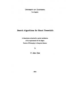
List of Figures 5.1 Meaning of vector Rj in the Shift-Or algorithm. 38 6.1 Shift in the Morris-Pratt algorithm: v is the border of u. 42 7.1 Shift in the Knuth-Morris-Pratt algorithm: v is a border of u and a 6= c. 48 9.1 Mismatch with a nohole. Noholes are black circles and are compared from left to right. In this situation, after the shift, it is not necessary to compare the rst two noholes again. 62 9.2 Mismatch with a hole. Noholes are black circles and are compared from left to right while holes are white circles and are compared from right to left. In this situation, after the shift, it is not necessary to compare the matched prex of the pattern again. 63 11.1 At each attempt of the Apostolico-Crochemore algorithm we consider a triple (i; j; k). 75 14.1 The good-sux shift, u re-occurs preceded by a character c dierent from a. 92 14.2 The good-sux shift, only a sux of u re-occurs in x. 92 14.3 The bad-character shift, a occurs in x. 92 14.4 The bad-character shift, a does not occur in x. 93 15.1 A turbo-shift can apply when jvj < juj. 100 15.2 c 6= d so they cannot be aligned with the same character in v. 100 16.1 Case 1, k > su [i] and su [i] = i + 1, an occurrence of x is found. 106 16.2 Case 2, k > su [i] and su [i] i, a mismatch occurs between y[i + j ? su [i]] and x[i ? su [i]]. 106

9

10

LIST OF FIGURES 16.3 Case 3, k < su [i] a mismatch occurs between y[i+j ? k] and x[i ? k]. 106 16.4 Case 4, k = su [i]anda 6= b. 106 26.1 Impossible overlap if z is an acyclic word. 28.1 A perfect factorization of x.

152

164

30.1 Typical attempt during the String Matching on Ordered Alphabets algorithm. 179 30.2 Function nextMaximalSuffix: meaning of the variables i, j, k and p. 180 34.1 General situation during the searching phase of the KmpSkip algorithm. 200

1

Introduction

String-matching is a very important subject in the wider domain of text processing. String-matching algorithms are basic components used in implementations of practical softwares existing under most operating systems. Moreover, they emphasize programming methods that serve as paradigms in other elds of computer science (system or software design). Finally, they also play an important role in theoretical computer science by providing challenging problems. Although data are memorized in various ways, text remains the main form to exchange information. This is particularly evident in literature or linguistics where data are composed of huge corpus and dictionaries. This apply as well to computer science where a large amount of data are stored in linear les. And this is also the case, for instance, in molecular biology because biological molecules can often be approximated as sequences of nucleotides or amino acids. Furthermore, the quantity of available data in these elds tend to double every eighteen months. This is the reason why algorithms should be ecient even if the speed and capacity of storage of computers increase regularly. String-matching consists in nding one, or more generally, all the occurrences of a string (more generally called a pattern) in a text. All the algorithms in this book output all occurrences of the pattern in the text. The pattern is denoted by x = x[0 : :m ? 1]; its length is equal to m. The text is denoted by y = y[0 : :n ? 1]; its length is equal to n. Both strings are build over a nite set of character called an alphabet denoted by with size is equal to . Applications require two kinds of solution depending on which string, the pattern or the text, is given rst. Algorithms based on the use of automata or combinatorial properties of strings are commonly implemented to preprocess the pattern and solve the rst kind of problem. The notion of indexes realized by trees or automata is used in the second kind of solutions. This book will only investigate algorithms of the rst kind. String-matching algorithms of the present book work as follows. They

12

Chapter 1 Introduction scan the text with the help of a window which size is generally equal to m. They rst align the left ends of the window and the text, then compare the characters of the window with the characters of the pattern this specic work is called an attempt and after a whole match of the pattern or after a mismatch they shift the window to the right. They repeat the same procedure again until the right end of the window goes beyond the right end of the text. This mechanism is usually called the sliding window mechanism. We associate each attempt with the position j in the text when the window is positioned on y[j : :j +m ? 1]. The brute force algorithm locates all occurrences of x in y in time O(m n). The many improvements of the brute force method can be classied depending on the order they performed the comparisons between pattern characters and text characters et each attempt. Four categories arise: the most natural way to perform the comparisons is from left to right, which is the reading direction; performing the comparisons from right to left generally leads to the best algorithms in practice; the best theoretical bounds are reached when comparisons are done in a specic order; nally there exist some algorithms for which the order in which the comparisons are done is not relevant (such is the brute force algorithm).

1.1

From left to right Hashing provides a simple method that avoids the quadratic number of character comparisons in most practical situations, and that runs in linear time under reasonable probabilistic assumptions. It has been introduced by Harrison and later fully analyzed by Karp and Rabin. Assuming that the pattern length is no longer than the memory-word size of the machine, the Shift-Or algorithm is an ecient algorithm to solve the exact string-matching problem and it adapts easily to a wide range of approximate string-matching problems. The rst linear-time string-matching algorithm is from Morris and Pratt. It has been improved by Knuth, Morris, and Pratt. The search behaves like a recognition process by automaton, and a character of the text is compared to a character p of the pattern no more than log (m+1) ( is the golden ratio (1 + 5)=2). Hancart proved that this delay of a related algorithm discovered by Simon makes no more than 1 + log2 m comparisons per text character. Those three algorithms perform at most 2n ? 1 text character comparisons in the worst case. The search with a Deterministic Finite Automaton performs exactly n text character inspections but it requires an extra space in O(m). The Forward Dawg Matching algorithm performs exactly the same number of text character inspections using the sux automaton of the pattern. The Apostolico-Crochemore algorithm is a simple algorithm which

1.2 From right to left

13

performs 23 n text character comparisons in the worst case. The Not So Naive algorithm is a very simple algorithm with a qua/dra/-tic worst case time complexity but it requires a preprocessing phase in constant time and space and is slightly sub-linear in the average case.

1.2

From right to left The Boyer-Moore algorithm is considered as the most ecient stringmatching algorithm in usual applications. A simplied version of it (or the entire algorithm) is often implemented in text editors for the search and substitute commands. Cole proved that the maximum number of character comparisons is tightly bounded by 3n after the preprocessing for non-periodic patterns. It has a quadratic worst case time for periodic patterns. Several variants of the Boyer-Moore algorithm avoid its quadratic behaviour. The most ecient solutions in term of number of character comparisons have been designed by Apostolico and Giancarlo, Crochemore et alii (Turbo-BM), and Colussi (Reverse Colussi). Empirical results show that variations of the Boyer-Moore algorithm and algorithms based on the sux automaton by Crochemore et alii (Reverse Factor and Turbo Reverse Factor) or the sux oracle by Crochemore et alii (Backward Oracle Matching) are the most ecient in practice. The Zhu-Takaoka and Berry-Ravindran algorithms are variants of the Boyer-Moore algorithm which require an extra space in O(2 ).

1.3

In a specic order The two rst linear optimal space string-matching algorithms are due to Galil-Seiferas and Crochemore-Perrin (Two Way). They partition the pattern in two parts, they rst search for the right part of the pattern from left to right and then if no mismatch occurs they search for the left part. The algorithms of Colussi and Galil-Giancarlo partition the set of pattern positions into two subsets. They rst search for the pattern characters which positions are in the rst subset from left to right and then if no mismatch occurs they search for the remaining characters from left to right. The Colussi algorithm is an improvement over the Knuth-Morris-Pratt algorithm and performs at most 23 n text character comparisons in the worst case. The Galil-Giancarlo algorithm improves the Colussi algorithm in one special case which enables it to perform at most 34 n text character comparisons in the worst case. Sunday's Optimal Mismatch and Maximal Shift algorithms sort the pattern positions according their character frequency and their leading

14

Chapter 1 Introduction shift respectively. Skip Search, KmPSkip Search and Alpha Skip Search algorithms by Charras et alii use buckets to determine starting positions on the pattern in the text.

1.4

In any order The Horspool algorithm is a variant of the Boyer-Moore algorithm, it uses only one of its shift functions and the order in which the text character comparisons are performed is irrelevant. This is also true for other variants such as the Quick Search algorithm of Sunday, Tuned BoyerMoore of Hume and Sunday, the Smith algorithm and the Raita algorithm.

1.5

Conventions We will consider practical searches. We will assume that the alphabet is the set of ASCII codes or any subset of it. The algorithms are presented in C programming language, thus a word w of length ` can be written w[0 : :` ? 1]; the characters are w[0]; : : :; w[` ? 1] and w[`] contained the special end character (null character) that cannot occur anywhere within any word but in the end. Both words the pattern and the text reside in main memory. Let us introduce some denitions.

Denitions

A word u is a prex of a word w is there exists a word v (possibly empty) such that w = uv. A word v is a sux of a word w is there exists a word u (possibly empty) such that w = uv. A word z is a substring or a subword or a factor of a word w is there exist two words u and v (possibly empty) such that w = uzv. A integer p is a period of a word w if for i, 0 i < m ? p, w[i] = w[i+p]. The smallest period of w is called the period of w, it is denoted by per(w). A word w of length ` is periodic if the length of its smallest period is smaller or equal to `=2, otherwise it is non-periodic . A word w is basic if it cannot be written as a power of another word: there exist no word z and no integer k such that w = z k . A word z is a border of a word w if there exist two words u and v such that w = uz = zv, z is both a prex and a sux of w. Note that in this case juj = jvj is a period of w.

1.5 Conventions

15

The reverse of a word w of length ` denoted by wR is the mirror image of w: wR = w[` ? 1]w[` ? 2] : : :w[1]w[0]. A Deterministic Finite Automaton (DFA) A is a quadruple (Q; q0; T; E) where: Q is a nite set of states; q0 2 Q is the initial state; T Q is the set of terminal states; E (Q Q) is the set of transitions. The language L(A) dened by A is the following set: fw 2 : 9q0; : : :; qn; n = jwj; qn 2 T; 80 i < n; (qi; w[i]; qi+1) 2 E g For each exact string-matching algorithm presented in the present book we rst give its main features, then we explained how it works before giving its C code. After that we show its behaviour on a typical example where x = GCAGAGAG and y = GCATCGCAGAGAGTATACAGTACG. Finally we give a list of references where the reader will nd more detailed presentations and proofs of the algorithm. At each attempt, matches are materialized in light gray while mismatches are shown in dark gray. A number indicates the order in which the character comparisons are done except for the algorithms using automata where the number represents the state reached after the character inspection.

Implementations In this book, we will use classical tools. One of them is a linked list of integer. It will be dened in C as follows: struct _cell { int element; struct _cell *next; }; typedef struct _cell *List;

Another important structures are tries and automata, specically sufx automata (see chapter 25). Basically automata are directed graphs. We will use the following interface to manipulate automata (assuming that vertices will be associated with positive integers): /* returns a new data structure for a graph with v vertices and e edges */ Graph newGraph(int v, int e); /* returns a new data structure for a automaton with v vertices and e edges */ Graph newAutomaton(int v, int e);

16

Chapter 1 Introduction /* returns a new data structure for a suffix automaton with v vertices and e edges */ Graph newSuffixAutomaton(int v, int e); /* returns a new data structure for a trie with v vertices and e edges */ Graph newTrie(int v, int e); /* returns a new vertex for graph g */ int newVertex(Graph g); /* returns the initial vertex of graph g */ int getInitial(Graph g); /* returns true if vertex v is terminal in graph g */ boolean isTerminal(Graph g, int v); /* set vertex v to be terminal in graph g */ void setTerminal(Graph g, int v); /* returns the target of edge from vertex v labelled by character c in graph g */ int getTarget(Graph g, int v, unsigned char c); /* add the edge from vertex v to vertex t labelled by character c in graph g */ void setTarget(Graph g, int v, unsigned char c, int t); /* returns the suffix link of vertex v in graph g */ int getSuffixLink(Graph g, int v); /* set the suffix link of vertex v to vertex s in graph g */ void setSuffixLink(Graph g, int v, int s); /* returns the length of vertex v in graph g */ int getLength(Graph g, int v); /* set the length of vertex v to integer ell in graph g */ void setLength(Graph g, int v, int ell); /* returns the position of vertex v in graph g */ int getPosition(Graph g, int v);

1.5 Conventions

17

/* set the length of vertex v to integer ell in graph g */ void setPosition(Graph g, int v, int p); /* returns the shift of the edge from vertex v labelled by character c in graph g */ int getShift(Graph g, int v, unsigned char c); /* set the shift of the edge from vertex v labelled by character c to integer s in graph g */ void setShift(Graph g, int v, unsigned char c, int s); /* copies all the characteristics of vertex source to vertex target in graph g */ void copyVertex(Graph g, int target, int source);

A possible implementation is given in appendix A.

2

Brute force algorithm

2.1

Main features

2.2

no preprocessing phase; constant extra space needed; always shifts the window by exactly 1 position to the right; comparisons can be done in any order; searching phase in O(m n) time complexity; 2n expected text character comparisons.

Description The brute force algorithm consists in checking, at all positions in the text between 0 and n ? m, whether an occurrence of the pattern starts there or not. Then, after each attempt, it shifts the pattern by exactly one position to the right. The brute force algorithm requires no preprocessing phase, and a constant extra space in addition to the pattern and the text. During the searching phase the text character comparisons can be done in any order. The time complexity of this searching phase is O(m n) (when searching for am?1 b in an for instance). The expected number of text character comparisons is 2n.

20

Chapter 2 Brute force algorithm

2.3

The C code void BF(char *x, int m, char *y, int n) { int i, j; /* Searching */ for (j = 0; j = m) OUTPUT(j); } }

This algorithm can be rewriting to give a more ecient algorithm in practice as follows: #define EOS '\0' void BF(char *x, int m, char *y, int n) { char *yb; /* Searching */ for (yb = y; *y != EOS; ++y) if (memcmp(x, y, m) == 0) OUTPUT(y - yb); }

However code optimization is beyond the scope of this book.

2.4

The example

Searching phase

First attempt: y

G C A T C G C A G A G A G T A T A C A G T A C G

x

G C A G A G A G

1 2 3 4

Shift by 1

2.4 The example

21

Second attempt: y


x

1 G C A G A G A G

Shift by 1 Third attempt: y

G C A T C G C A G A G A G T A T A C A G T A C G 1

x

G C A G A G A G

Shift by 1 Fourth attempt: y


x

1 G C A G A G A G

Shift by 1

Fifth attempt: y


Shift by 1

1

x

G C A G A G A G

Sixth attempt: y


Shift by 1

x

1 2 3 4 5 6 7 8 G C A G A G A G

Seventh attempt: y


Shift by 1

x

1 G C A G A G A G

22

Chapter 2 Brute force algorithm Eighth attempt: y


Shift by 1

x

1 G C A G A G A G

Ninth attempt: y


Shift by 1

x

1 2 G C A G A G A G

Tenth attempt: y


Shift by 1

x

1 G C A G A G A G

Eleventh attempt: y


Shift by 1

x

1 2 G C A G A G A G

Twelfth attempt: y


Shift by 1

x

1 G C A G A G A G

Thirteenth attempt: y


Shift by 1

x

1 2 G C A G A G A G

2.4 The example

23

Fourteenth attempt: y


Shift by 1

x

1 G C A G A G A G

Fifteenth attempt: y


Shift by 1

x

1 G C A G A G A G

Sixteenth attempt: y


Shift by 1

x

1 G C A G A G A G

Seventeenth attempt: y


Shift by 1

x

1 G C A G A G A G

The brute force algorithm performs 30 text character comparisons on the example.

3

Search with an automaton

3.1

Main features

3.2

builds the minimal Deterministic Finite Automaton recognizing the language x; extra space in O(m ) if the automaton is stored in a direct access table; preprocessing phase in O(m ) time complexity; searching phase in O(n) time complexity if the automaton is stored in a direct access table, O(n log ) otherwise.

Description Searching a word x with an automaton consists rst in building the minimal Deterministic Finite Automaton (DFA) A(x) recognizing the language x. The DFA A(x) = (Q; q0; T; E) recognizing the language x is dened as follows: Q is the set of all the prexes of x: Q = f"; x[0]; x[0 ::1]; : : :; x[0 : :m ? 2]; xg , q0 = " , T = fxg , for q 2 Q (q is a prex of x) and a 2 , (q; a; qa) 2 E if and only if qa is also a prex of x, otherwise (q; a; p) 2 E such that p is the longest sux of qa which is a prex of x. The DFA A(x) can be constructed in O(m + ) time and O(m ) space. Once the DFA A(x) is build, searching for a word x in a text y consists in parsing the text y with the DFA A(x) beginning with the initial state

26

Chapter 3 Search with an automaton q0. Each time the terminal state is encountered an occurrence of x is reported. The searching phase can be performed in O(n) time if the automaton is stored in a direct access table, in O(n log ) otherwise.

3.3

The C code void preAut(char *x, int m, Graph aut) { int i, state, target, oldTarget; for (state = getInitial(aut), i = 0; i < m; ++i) { oldTarget = getTarget(aut, state, x[i]); target = newVertex(aut); setTarget(aut, state, x[i], target); copyVertex(aut, target, oldTarget); state = target; } setTerminal(aut, state); }

void AUT(char *x, int m, char *y, int n) { int j, state; Graph aut; /* Preprocessing */ aut = newAutomaton(m + 1, (m + 1)*ASIZE); preAut(x, m, aut); /* Searching */ for (state = getInitial(aut), j = 0; j < n; ++j) { state = getTarget(aut, state, y[j]); if (isTerminal(aut, state)) OUTPUT(j - m + 1); } }

3.4 The example

3.4

27

The example = fA; C; G; Tg Q = f"; G; GC; GCA; GCAG; GCAGA; GCAGAG; GCAGAGA; GCAGAGAGg q0 = " T = fGCAGAGAGg

C C C

G

0

G

1

C

2

A

3

G

4

A

5

G

6

A

7

G

G G G G

The states are labelled by the length of the prex they are associated with. Missing transitions are leading to the initial state 0.

Searching phase The initial state is 0. y


8

28

Chapter 3 Search with an automaton y


y


y


y


y


y


y


y


y


y


3.4 The example y

29


y


y


y


y


y


y


y


y


y


30

Chapter 3 Search with an automaton y


y


y


The search by automaton performs exactly 24 text character inspections on the example.

3.5

References

Cormen, T.H., Leiserson, C.E., Rivest, R.L., 1990, Introduc-

tion to Algorithms, Chapter 34, pp 853885, MIT Press. Crochemore, M., 1997, O-line serial exact string searching, in Pattern Matching Algorithms, A. Apostolico and Z. Galil ed., Chapter 1, pp 153, Oxford University Press. Crochemore, M., Hancart, C., 1997, Automata for Matching Patterns, in Handbook of Formal Languages, Volume 2, Linear Modeling: Background and Application, G. Rozenberg and A. Salomaa ed., Chapter 9, pp 399462, Springer-Verlag, Berlin. Gonnet, G.H., Baeza-Yates, R.A., 1991, Handbook of Algorithms and Data Structures in Pascal and C, 2nd Edition, Chapter 7, pp. 251288, Addison-Wesley Publishing Company. Hancart, C., 1993, Analyse exacte et en moyenne d'algorithmes de recherche d'un motif dans un texte, Thèse de doctorat de l'Université de Paris 7, France.

4

Karp-Rabin algorithm

4.1

Main features

4.2

uses an hashing function; preprocessing phase in O(m) time complexity and constant space; searching phase in O(m n) time complexity; O(m + n) expected running time.

Description Hashing provides a simple method to avoid a quadratic number of character comparisons in most practical situations. Instead of checking at each position of the text if the pattern occurs, it seems to be more ecient to check only if the contents of the window looks like the pattern. In order to check the resemblance between these two words an hashing function is used. To be helpful for the string matching problem an hashing function hash should have the following properties: eciently computable; highly discriminating for strings; hash(y[j+1 : :j+m]) must be easily computable from hash(y[j : :j+ m ? 1]) and y[j + m]: hash(y[j + 1 : :j + m]) = rehash(y[j]; y[j + m]; hash(y[j : :j + m ? 1])) . For a word w of length m let hash(w) be dened as follows: hash(w[0 : :m ? 1]) = (w[0] 2m?1 + w[1] 2m?2 + + w[m ? 1] 20 ) mod q where q is a large number. Then, rehash(a; b; h) = ((h ? a 2m?1) 2 + b) mod q .

32

Chapter 4 Karp-Rabin algorithm The preprocessing phase of the Karp-Rabin algorithm consists in computing hash(x). It can be done in constant space and O(m) time. During the searching phase, it is enough to compare hash(x) with hash(y[j : :j + m ? 1]) for 0 j n ? m. If an equality is found, it is still necessary to check the equality x = y[j : :j + m ? 1] character by character. The time complexity of the searching phase of the Karp-Rabin algorithm is O(m n) (when searching for am in an for instance). Its expected number of text character comparisons is O(m + n).

4.3

The C code In the following function KR all the multiplications by 2 are implemented by shifts. Furthermore, the computation of the modulus function is avoided by using the implicit modular arithmetic given by the hardware that forgets carries in integer operations. So, q is chosen as the maximum value for an integer. #define REHASH(a, b, h) ((((h) - (a)*d) -1 && x[i] != x[j]) j = kmpNext[j]; i++; j++; if (x[i] == x[j]) kmpNext[i] = kmpNext[j]; else kmpNext[i] = j; } }

void KMP(char *x, int m, char *y, int n) { int i, j, kmpNext[XSIZE]; /* Preprocessing */ preKmp(x, m, kmpNext);

7.4 The example /* Searching */ i = j = 0; while (j < n) { while (i > -1 && x[i] != y[j]) i = kmpNext[i]; i++; j++; if (i >= m) { OUTPUT(j - i); i = kmpNext[i]; } } }

7.4

The example

i 0 1 2 3 4 5 6 7 8 x[i] G C A G A G A G kmpNext[i] ?1 0 0 ?1 1 ?1 1 ?1 1

Searching phase First attempt: y


x

G C A G A G A G

1 2 3 4

Shift by 4 (i ? kmpNext[i] = 3 ? ?1) Second attempt: y


x

1 G C A G A G A G

Shift by 1 (i ? kmpNext[i] = 0 ? ?1) Third attempt: y


x

1 2 3 4 5 6 7 8 G C A G A G A G

Shift by 7 (i ? kmpNext[i] = 8 ? 1)

49

50

Chapter 7 Knuth-Morris-Pratt algorithm Fourth attempt: y


x

2 G C A G A G A G

Shift by 1 (i ? kmpNext[i] = 1 ? 0) Fifth attempt: y


x

1 G C A G A G A G

Shift by 1 (i ? kmpNext[i] = 0 ? ?1) Sixth attempt: y


x

Shift by 1 (i ? kmpNext[i] = 0 ? ?1)

G C A G A G A G

Seventh attempt: y


x


1 G C A G A G A G

Eighth attempt: y



x

1 G C A G A G A G

The Knuth-Morris-Pratt algorithm performs 18 text character comparisons on the example.

7.5

References

Aho, A.V., 1990, Algorithms for Finding Patterns in Strings, in Handbook of Theoretical Computer Science, Volume A, Algorithms

7.5 References

51

and complexity, J. van Leeuwen ed., Chapter 5, pp 255300, Elsevier, Amsterdam. Aoe, J.-I., 1994, Computer algorithms: string pattern matching strategies, IEEE Computer Society Press. Baase, S., Van Gelder, A., 1999, Computer Algorithms: Introduction to Design and Analysis, 3rd Edition, Chapter 11, AddisonWesley Publishing Company. Baeza-Yates, R.A., Navarro G., Ribeiro-Neto B., 1999, Indexing and Searching, in Modern Information Retrieval, Chapter 8, pp 191228, Addison-Wesley. Beauquier, D., Berstel, J., Chrétienne, P., 1992, Éléments d'algorithmique, Chapter 10, pp 337377, Masson, Paris. Cormen, T.H., Leiserson, C.E., Rivest, R.L., 1990, Introduction to Algorithms, Chapter 34, pp 853885, MIT Press. Crochemore, M., 1997, O-line serial exact string searching, in Pattern Matching Algorithms, A. Apostolico and Z. Galil ed., Chapter 1, pp 153, Oxford University Press. Crochemore, M., Hancart, C., 1999, Pattern Matching in Strings, in Algorithms and Theory of Computation Handbook, M.J. Atallah ed., Chapter 11, pp 11-111-28, CRC Press Inc., Boca Raton, FL. Crochemore, M., Lecroq, T., 1996, Pattern matching and text compression algorithms, in CRC Computer Science and Engineering Handbook, A.B. Tucker Jr ed., Chapter 8, pp 162202, CRC Press Inc., Boca Raton, FL. Crochemore, M., Rytter, W., 1994, Text Algorithms, Oxford University Press. Gonnet, G.H., Baeza-Yates, R.A., 1991, Handbook of Algorithms and Data Structures in Pascal and C, 2nd Edition, Chapter 7, pp. 251288, Addison-Wesley Publishing Company. Goodrich, M.T., Tamassia, R., 1998, Data Structures and Algorithms in JAVA, Chapter 11, pp 441467, John Wiley & Sons. Gusfield, D., 1997, Algorithms on strings, trees, and sequences: Computer Science and Computational Biology, Cambridge University Press. Hancart, C., 1992, Une analyse en moyenne de l'algorithme de Morris et Pratt et de ses ranements, in Théorie des Automates et Applications, Actes des 2e Journées Franco-Belges, D. Krob ed., Rouen, France, pp 99110, PUR 176, Rouen, France. Hancart, C., 1993, Analyse exacte et en moyenne d'algorithmes de recherche d'un motif dans un texte, Thèse de doctorat de l'Université de Paris 7, France.

52

Chapter 7 Knuth-Morris-Pratt algorithm

Knuth, D.E., Morris, Jr, J.H., Pratt, V.R., 1977, Fast pattern matching in strings, SIAM Journal on Computing 6(1):323 350. Sedgewick, R., 1988, Algorithms, Chapter 19, pp. 277292, Addison-Wesley Publishing Company. Sedgewick, R., 1992, Algorithms in C, Chapter 19, AddisonWesley Publishing Company. Sedgewick, R., Flajolet, P., 1996, An Introduction to the Analysis of Algorithms, Chapter 7, Addison-Wesley Publishing Company. Stephen, G.A., 1994, String Searching Algorithms, World Scientic. Watson, B.W., 1995, Taxonomies and Toolkits of Regular Language Algorithms, PhD Thesis, Eindhoven University of Technology, The Netherlands. Wirth, N., 1986, Algorithms & Data Structures, Chapter 1, pp. 1772, Prentice-Hall.

8

Simon algorithm

8.1

Main features

8.2

economical implementation of A(x) the minimal Deterministic Finite Automaton recognizing x; preprocessing phase in O(m) time and space complexity; searching phase in O(m+n) time complexity (independent from the alphabet size); at most 2n ? 1 text character comparisons during the searching phase; delay bounded by minf1 + log2 m; g.

Description The main drawback of the search with the minimal DFA A(x) (see chapter 3) is the size of the automaton: O(m ). Simon noticed that there are only a few signicant edges in A(x); they are: the forward edges going from the prex of x of length k to the prex of length k + 1 for 0 k < m. There are exactly m such edges; the backward edges going from the prex of x of length k to a smaller non-zero length prex. The number of such edges is bounded by m. The other edges are leading to the initial state and can then be deduced. Thus the number of signicant edges is bounded by 2m. Then for each state of the automaton it is only necessary to store the list of its signicant outgoing edges. Each state is represented by the length of its associated prex minus 1 in order that each edge leading to state i, with ?1 i m ? 1 is labelled by x[i] thus it is not necessary to store the labels of the edges. The forward edges can be easily deduced from the pattern, thus they are not stored. It only remains to store the signicant backward edges.

54

Chapter 8 Simon algorithm We use a table L, of size m ? 2, of linked lists. The element L[i] gives the list of the targets of the edges starting from state i. In order to avoid to store the list for the state m ? 1, during the computation of this table L, the integer ` is computed such that ` + 1 is the length of the longest border of x. The preprocessing phase of the Simon algorithm consists in computing the table L and the integer `. It can be done in O(m) space and time complexity. The searching phase is analogous to the one of the search with an automaton. When an occurrence of the pattern is found, the current state is updated with the state `. This phase can be performed in O(m+ n) time. The Simon algorithm performs at most 2n ? 1 text character comparisons during the searching phase. The delay (maximal number of comparisons for a single text character) is bounded by minf1+log2 m; g.

8.3

The C code The description of a linked list List can be found section 1.5. int getTransition(char *x, int m, int p, List L[], char c) { List cell; if (p < m - 1 && x[p + 1] == c) return(p + 1); else if (p > -1) { cell = L[p]; while (cell != NULL) if (x[cell->element] == c) return(cell->element); else cell = cell->next; return(-1); } else return(-1); }

void setTransition(int p, int q, List L[]) { List cell; cell = (List)malloc(sizeof(struct _cell)); if (cell == NULL) error("SIMON/setTransition");

8.3 The C code cell->element = q; cell->next = L[p]; L[p] = cell; }

int preSimon(char *x, int m, List L[]) { int i, k, ell; List cell; memset(L, NULL, (m - 2)*sizeof(List)); ell = -1; for (i = 1; i < m; ++i) { k = ell; cell = (ell == -1 ? NULL : L[k]); ell = -1; if (x[i] == x[k + 1]) ell = k + 1; else setTransition(i - 1, k + 1, L); while (cell != NULL) { k = cell->element; if (x[i] == x[k]) ell = k; else setTransition(i - 1, k, L); cell = cell->next; } } return(ell); }

void SIMON(char *x, int m, char *y, int n) { int j, ell, state; List L[XSIZE]; /* Preprocessing */ ell = preSimon(x, m, L); /* Searching */ for (state = -1, j = 0; j < n; ++j) { state = getTransition(x, m, state, L, y[j]); if (state >= m - 1) { OUTPUT(j - m + 1);

55

56

Chapter 8 Simon algorithm state = ell; } } }

8.4

The example C C

G

-1

G

C

0

1

A

2

G

3

A

4

G

5

A

6

G

7

G G G

The states are labelled by the length of the prex they are associated with minus 1. i 0 1 2 3 4 5 6 L[i] (0) (0) ; (0; 1) ; (0; 1) ;

Searching phase The initial state is ?1. y


y


y


8.4 The example

57

y


y


y


?1 ?1

0

y


y


y


y


y


y


y


58

Chapter 8 Simon algorithm y


y


y


y


y


y


y


?1 ?1 ?1 ?1 ?1 ?1

0

y


y


y


?1 ?1 ?1

8.5 References y

59


The Simon algorithm performs 24 text character comparisons on the example.

8.5

References

Beauquier, D., Berstel, J., Chrétienne, P., 1992, Éléments d'algorithmique, Chapter 10, pp 337377, Masson, Paris. Crochemore, M., 1997, O-line serial exact string searching, in Pattern Matching Algorithms, A. Apostolico and Z. Galil ed., Chapter 1, pp 153, Oxford University Press. Crochemore, M., Hancart, C., 1997, Automata for Matching Patterns, in Handbook of Formal Languages, Volume 2, Linear Modeling: Background and Application, G. Rozenberg and A. Salomaa ed., Chapter 9, pp 399462, Springer-Verlag, Berlin. Crochemore, M., Rytter, W., 1994, Text Algorithms, Oxford University Press. Hancart, C., 1992, Une analyse en moyenne de l'algorithme de Morris et Pratt et de ses ranements, in Théorie des Automates et Applications, Actes des 2e Journées Franco-Belges, D. Krob ed., Rouen, France, pp 99110, PUR 176, Rouen, France. Hancart, C., 1993, On Simon's string searching algorithm, Information Processing Letters 47(2):9599. Hancart, C., 1993, Analyse exacte et en moyenne d'algorithmes de recherche d'un motif dans un texte, Thèse de doctorat de l'Université de Paris 7, France. Simon, I., 1993, String matching algorithms and automata, in Proceedings of the 1st American Workshop on String Processing, R.A. Baeza-Yates and N. Ziviani ed., pp 151157, Universidade Federal de Minas Gerais, Brazil. Simon, I., 1994, String matching algorithms and automata, in Results and Trends in Theoretical Computer Science, Graz, Austria, J. Karhumäki, H. Maurer and G. Rozenberg ed., pp 386395, Lecture Notes in Computer Science 814, Springer-Verlag, Berlin.

9

Colussi algorithm

9.1

Main features

9.2

renement of the Knuth-Morris-Pratt algorithm; partitions the set of pattern positions into two disjoint subsets; the positions in the rst set are scanned from left to right and when no mismatch occurs the positions of the second subset are scanned from right to left; preprocessing phase in O(m) time and space complexity; searching phase in O(n) time complexity; performs 23 n text character comparisons in the worst case.

Description The design of the Colussi algorithm follows a tight analysis of the KnuthMorris-Pratt algorithm (see chapter 7). The set of pattern positions is divided into two disjoint subsets. Then each attempt consists in two phases: in the rst phase the comparisons are performed from left to right with text characters aligned with pattern position for which the value of the kmpNext function is strictly greater than ?1. These positions are called noholes ; the second phase consists in comparing the remaining positions (called holes ) from right to left. This strategy presents two advantages: when a mismatch occurs during the rst phase, after the appropriate shift it is not necessary to compare the text characters aligned with noholes compared during the previous attempt; when a mismatch occurs during the second phase it means that a sux of the pattern matches a factor of the text, after the corre-

62

Chapter 9 Colussi algorithm y x

x

Mismatch with a nohole. Noholes are black circles and are compared from left to right. In this situation, after the shift, it is not necessary to compare the rst two noholes again.

Figure 9.1

sponding shift a prex of the pattern will still match a factor of the text, then it is not necessary to compare this factor again. For 0 i m ? 1: ( d > 0 if and only if x[0 : :i ? 1 ? d] = x[d : :i ? 1] and kmin[i] = x[i ? d] 6= x[i] , 0 otherwise . When kmin[i] 6= 0 a periodicity ends at position i in x. For 0 < i < m if kmin[i ? 1] 6= 0 then i is a nohole otherwise i is a hole. Let nd + 1 be the number of noholes in x. The table h contains rst the nd + 1 noholes in increasing order and then the m ? nd ? 1 holes in decreasing order: for 0 i nd, h[i] is a nohole and h[i] < h[i + 1] for 0 i < nd; for nd < i < m, h[i] is a hole and h[i] > h[i + 1] for nd < i < m ? 1. If i is a hole then rmin[i] is the smallest period of x greater than i. The value of rst[u] is the smallest integer v such that u h[v]. Then assume that x is aligned with y[j : :j + m ? 1]. If x[h[k]] = y[j + h[k]] for 0 k < r < nd and x[h[r]] 6= y[j + h[r]]. Let j 0 = j + kmin[h[r]]. Then there is no occurrence of x beginning in y[j : :j 0 ] and x can be shifted by kmin[h[r]] positions to the right. Moreover x[h[k]] = y[j 0 + h[k]] for 0 k < rst[h[r] ? kmin[h[r]]] meaning that the comparisons can be resume with x[h[rst[h[r] ? kmin[h[r]]]]] and y[j 0 + h[rst[h[r] ? kmin[h[r]]]]] (see gure 9.1). If x[h[k]] = y[j + h[k]] for 0 k < r and x[h[r]] 6= y[j + h[r]] with nd r < m. Let j 0 = j + rmin[h[r]]. Then there is no occurrence of x beginning in y[j : :j 0 ] and x can be shifted by kmin[h[r]] positions to the right. Moreover x[0 : :m ? 1 ? rmin[h[r]]] = y[j 0 : :j + m ? 1] meaning that the comparisons can be resume with x[h[rst[m ? 1 ? rmin[h[r]]]]] and y[j 0 + h[rst[m ? 1 ? rmin[h[r]]]]] (see gure 9.2). To compute the values of kmin, a table hmax is used and dened as follows: hmax[k] is such that x[k : :hmax[k] ? 1] = x[0 : :hmax[k] ? k ? 1] and x[hmax[k]] 6= x[hmax[k] ? k]. The value of ndh0[i] is the number of noholes strictly smaller than i. We can now dene two functions shift and next as follows:

9.3 The C code y x

63

x

Figure 9.2 Mismatch with a hole. Noholes are black circles and are compared from left to right while holes are white circles and are compared from right to left. In this situation, after the shift, it is not necessary to compare the matched prex of the pattern again.

shift[i] = kmin[h[i]] and next[i] = ndh0[h[i] ? kmin[h[i]]] for i < nd; shift[i] = rmin[h[i]] and next[i] = ndh0[m ? rmin[h[i]]] for nd i < m; shift[m] = rmin[0] and next[m] = ndh0[m ? rmin[h[m ? 1]]]. Thus, during an attempt where the window is positioned on the text factor y[j : :j + m ? 1], when a mismatch occurs between x[h[r]] and y[j + h[r]] the window must be shifted by shift[r] and the comparisons can be resume with pattern position h[next[r]]. The preprocessing phase can be done in O(m) space and time. The searching phase can then be done in O(n) time complexity and furthermore at most 23 n text character comparisons are performed during the searching phase.

9.3

The C code int preColussi(char *x, int m, int h[], int next[], int shift[]) { int i, k, nd, q, r, s; int hmax[XSIZE], kmin[XSIZE], nhd0[XSIZE], rmin[XSIZE]; /* Computation of hmax */ i = k = 1; do { while (x[i] == x[i - k]) i++; hmax[k] = i; q = k + 1; while (hmax[q - k] + k < i) { hmax[q] = hmax[q - k] + k; q++; } k = q; if (k == i + 1)

64

Chapter 9 Colussi algorithm i = k; } while (k = 1; --i) if (hmax[i] < m) kmin[hmax[i]] = i; /* Computation of rmin */ for (i = m - 1; i >= 0; --i) { if (hmax[i + 1] == m) r = i + 1; if (kmin[i] == 0) rmin[i] = r; else rmin[i] = 0; } /* Computation of h */ s = -1; r = m; for (i = 0; i < m; ++i) if (kmin[i] == 0) h[--r] = i; else h[++s] = i; nd = s; /* Computation of shift */ for (i = 0; i 0) ++s; }

9.3 The C code /* Computation of next */ for (i = 0; i = j + h[i]) { OUTPUT(j); i = m; } if (i > nd) last = j + m - 1; j += shift[i]; i = next[i]; } }

65

66

Chapter 9 Colussi algorithm

9.4

The example i x[i] kmpNext[i] kmin[i] h[i] next[i] shift[i] hmax[i] rmin[i] ndh0[i] nd = 3

0 1 2 3 4 5 6 7 8

G

-1 0 1 0 1 0 7 0

C

0 1 2 0 2 1 0 0

A

0 2 4 0 3 2 0 1

G

-1 0 6 0 5 4 7 2

A

1 3 7 0 8 4 0 2

G

-1 0 5 0 7 6 7 3

A

1 5 3 0 7 6 0 3

G

-1 0 0 0 7 8 8 4

1 0 7 8


x

G C A T C G C A G A G A G T A T A C A G T A C G 1 2

3

G C A G A G A G

Shift by 3 (shift[2]) Second attempt: y


x

1 2 G C A G A G A G

Shift by 2 (shift[1]) Third attempt: y


x

8 1 2 7 3 6 4 5 G C A G A G A G

Shift by 7 (shift[8])

9.5 References

67

Fourth attempt: y



x

1 G C A G A G A G

Fifth attempt: y



x

1 G C A G A G A G

Sixth attempt: y



x

1 G C A G A G A G

Seventh attempt: y



x

1 G C A G A G A G

Eighth attempt: y



x

1 2

3

G C A G A G A G

The Colussi algorithm performs 20 text character comparisons on the example.

9.5

References

Breslauer, D., 1992, Ecient String Algorithmics, PhD Thesis,

Report CU02492, Computer Science Department, Columbia University, New York, NY.

68

Chapter 9 Colussi algorithm

Colussi, L., 1991, Correctness and eciency of the pattern matching algorithms, Information and Computation 95(2):225251. Colussi, L., Galil, Z., Giancarlo, R., 1990, On the exact complexity of string matching, in Proceedings of the 31st IEEE Annual Symposium on Foundations of Computer Science, Saint Louis, MO, pp 135144, IEEE Computer Society Press. Galil, Z., Giancarlo, R., 1992, On the exact complexity of string matching: upper bounds, SIAM Journal on Computing, 21 (3):407 437.

10

Galil-Giancarlo algorithm

10.1 Main features

renement of Colussi algorithm; preprocessing phase in O(m) time and space complexity; searching phase in O(n) time complexity; performs 43 n text character comparisons in the worst case.

10.2 Description The Galil-Giancarlo algorithm is a variant of the Colussi algorithm (see chapter 9). The change intervenes in the searching phase. The method applies when x is not a power of a single character. Thus x 6= cm with c 2 . Let ` be the last index in the pattern such that for 0 i `, x[0] = x[i] and x[0] 6= x[` + 1]. Assume that during the previous attempt all the noholes have been matched and a sux of the pattern has been matched meaning that after the corresponding shift a prex of the pattern will still match a part of the text. Thus the window is positioned on the text factor y[j : :j + m ? 1] and the portion y[j : :last] matches x[0 : :last ? j]. Then during the next attempt the algorithm will scanned the text character beginning with y[last+1] until either the end of the text is reached or a character x[0] 6= y[j + k] is found. In this latter case two subcases can arise: x[` + 1] 6= y[j + k] or too less x[0] have been found (k `) then the window is shifted and positioned on the text factor y[k +1 : :k +m], the scanning of the text is resumed (as in the Colussi algorithm) with the rst nohole and the memorized prex of the pattern is the empty word. x[` + 1] = y[j + k] and enough of x[0] has been found (k > `) then the window is shifted and positioned on the text factor y[k ? ` ? 1 : :k ? ` + m ? 2], the scanning of the text is resumed (as in the

70

Chapter 10 Galil-Giancarlo algorithm Colussi algorithm) with the second nohole (x[` + 1] is the rst one) and the memorized prex of the pattern is x[0 : :` + 1]. The preprocessing phase is exactly the same as in the Colussi algorithm (chapter 9) and can be done in O(m) space and time. The searching phase can then be done in O(n) time complexity and furthermore at most 34 n text character comparisons are performed during the searching phase.

10.3 The C code The function preColussi is given chapter 9. void GG(char *x, int m, char *y, int n) { int i, j, k, ell, last, nd; int h[XSIZE], next[XSIZE], shift[XSIZE]; char heavy; for (ell = 0; x[ell] == x[ell + 1]; ell++); if (ell == m - 1) /* Searching for a power of a single character */ for (j = ell = 0; j < n; ++j) if (x[0] == y[j]) { ++ell; if (ell >= m) OUTPUT(j - m + 1); } else ell = 0; else { /* Preprocessing */ nd = preCOLUSSI(x, m, h, next, shift); /* Searching */ i = j = heavy = 0; last = -1; while (j = j + h[i]) { OUTPUT(j); i = m; } if (i > nd) last = j + m - 1; j += shift[i]; i = next[i]; } heavy = (j > last ? 0 : 1); } } }

10.4 The example i 0 x[i] G kmpNext[i] -1 kmin[i] 0 h[i] 1 next[i] 0 shift[i] 1 hmax[i] 0 rmin[i] 7 ndh0[i] 0 nd = 3 and ` = 0

1 2 3 4 5 6 7 8

C

0 1 2 0 2 1 0 0

A

0 2 4 0 3 2 0 1

G

-1 0 6 0 5 4 7 2

A

1 3 7 0 8 4 0 2

G

-1 0 5 0 7 6 7 3

A

1 5 3 0 7 6 0 3

G

-1 0 0 0 7 8 8 4

1 0 7 8

72

Chapter 10 Galil-Giancarlo algorithm



x

G C A G A G A G

1 2

3

Shift by 3 (shift[2]) Second attempt: y


x

1 2 G C A G A G A G

Shift by 2 (shift[1]) Third attempt: y


x

8 1 2 7 3 6 4 5 G C A G A G A G

Shift by 7 (shift[8]) Fourth attempt: y


Shift by 2

x

1 G

Fifth attempt: y



x

1 G C A G A G A G

Sixth attempt: y



x

1 G C A G A G A G

10.5 References

73

Seventh attempt: y



x

1 2

3

G C A G A G A G

The Galil-Giancarloalgorithm performs 19 text character comparisons on the example.

10.5 References

Breslauer, D., 1992, Ecient String Algorithmics, PhD Thesis,

Report CU02492, Computer Science Department, Columbia University, New York, NY. Galil, Z., Giancarlo, R., 1992, On the exact complexity of string matching: upper bounds, SIAM Journal on Computing, 21 (3):407 437.

11

Apostolico-Crochemore algorithm

11.1 Main features

preprocessing phase in O(m) time and space complexity; searching phase in O(n) time complexity; performs 32 n text character comparisons in the worst case.

11.2 Description The Apostolico-Crochemore uses the kmpNext shift table (see chapter 7) to compute the shifts. Let ` = 0 if x is a power of a single character (x = cm with c 2 ) and ` be equal to the position of the rst character of x dierent from x[0] otherwise (x = a` bu for a; b 2 , u 2 and a 6= b). During each attempt the comparisons are made with pattern positions in the following order: `; ` + 1; : : :; m ? 2; m ? 1; 0; 1; : ::; ` ? 1. During the searching phase we consider triple of the form (i; j; k) where: the window is positioned on the text factor y[j : :j + m ? 1]; 0 k ` and x[0 : :k ? 1] = y[j : :j + k ? 1]; ` i < m and x[` : :i ? 1] = y[j + ` : :i + j ? 1]. (see gure 11.1). The initial triple is (`; 0; 0). y x

j

j+k

0

k

i+j j+m?1

`

i

Figure 11.1 At each attempt of the Apostolico-Crochemore algorithm we consider a triple (i; j; k).

76

Chapter 11 Apostolico-Crochemore algorithm We now explain how to compute the next triple after (i; j; k) has been computed. Three cases arise depending on the value of i: i=` If x[i] = y[i + j] then the next triple is (i + 1; j; k). If x[i] 6= y[i + j] then the next triple is (`; j + 1; maxf0; k ? 1g). `= ell) OUTPUT(j); } j += (i - kmpNext[i]); if (i == ell) k = MAX(0, k - 1); else if (kmpNext[i] 0 : Cs(i; s) and Co(i; s) holdg y x x Figure 14.3

b a b

u u

shift contains no b

The bad-character shift, a occurs in x.

14.3 The C code

93

y

b a

x x Figure 14.4

u u

shift contains no b

The bad-character shift, a does not occur in x.

and we dene bmGs[0] as the length of the period of x. The computation of the table bmGs use a table su dened as follows: for 1 i < m; su [i] = maxfk : x[i ? k + 1 : :i] = x[m ? k; m ? 1]g . The bad-character shift function is stored in a table bmBc of size . For c 2 : ( minfi : 1 i < m ? 1 and x[m ? 1 ? i] = cg if c occurs bmBc[c] = in x , m otherwise . Tables bmBc and bmGs can be precomputed in time O(m+) before the searching phase and require an extra-space in O(m+). The searching phase time complexity is quadratic but at most 3n text character comparisons are performed when searching for a non periodic pattern. On large alphabets (relatively to the length of the pattern) the algorithm is extremely fast. When searching for am?1 b in an the algorithm makes only O(n=m) comparisons, which is the absolute minimum for any string-matching algorithm in the model where the pattern only is preprocessed.

14.3 The C code void preBmBc(char *x, int m, int bmBc[]) { int i; for (i = 0; i < ASIZE; ++i) bmBc[i] = m; for (i = 0; i < m - 1; ++i) bmBc[x[i]] = m - i - 1; }

void suffixes(char *x, int m, int *suff) { int f, g, i; suff[m - 1] = m;

94

Chapter 14 Boyer-Moore algorithm g = m - 1; for (i = m - 2; i >= 0; --i) { if (i > g && suff[i + m - 1 - f] < i - g) suff[i] = suff[i + m - 1 - f]; else { if (i < g) g = i; f = i; while (g >= 0 && x[g] == x[g + m - 1 - f]) --g; suff[i] = f - g; } } } void preBmGs(char *x, int m, int bmGs[]) { int i, j, suff[XSIZE]; suffixes(x, m, suff); for (i = 0; i < m; ++i) bmGs[i] = m; j = 0; for (i = m - 1; i >= -1; --i) if (i == -1 || suff[i] == i + 1) for (; j < m - 1 - i; ++j) if (bmGs[j] == m) bmGs[j] = m - 1 - i; for (i = 0; i