Temperature Driven Time Synchronization - Semantic Scholar

1

Temperature Driven Time Synchronization Thomas Schmid, Zainul Charbiwala, Roy Shea, Mani B. Srivastava Electrical Engineering Department University of California, Los Angeles {thomas.schmid, zainul, rshea, mbs}@ucla.edu

Abstract—Time synchronization in embedded sensor networks is an important service for correlating data between nodes and communication scheduling. While many different approaches to the problem are possible, one major effect of clock frequency difference between nodes, environmental temperature changes, has often been left out of the solution. The common assumption that the temperature is static over a certain period of time is often used as an excuse to assume constant frequency errors in a clock. This assumption forces synchronization protocols to resynchronize too often. While there exists hardware solutions to this problem, their prohibitive high cost and power consumption make them unsuitable for some applications, such as wireless sensor networks. Temperature Driven Time Synchronization (TDTS) exploits the onboard temperature sensor existing in many sensor network platforms. It uses this temperature sensor to autonomously calibrate the local oscillator and removes effects of environmental temperature changes. This allows a time synchronization protocol to increase its resynchronization period, without loosing synchronization accuracy, and thus saves energy and communication overhead. In addition, TDTS provides a stable clock source when radio communication is impaired. We present the theory behind TDTS, and provide initial results of a simulated comparison of TDTS and the Flooding Time Synchronization Protocol. Index Terms—synchronization; sensor networks; clocks

I. I NTRODUCTION Synchronizing two embedded systems over a wireless channel is a challenging problem. One has to consider several error sources including the accuracy of time stamping of a common event, message loss due to wireless channel fading and shadowing, and changes in the clock frequency due to environmental changes (temperature, acceleration, etc.). In addition to this, sensor networks add yet another challenge into the equation: energy efficiency. Several synchronization protocols have been proposed in recent years, addressing many of these problems. In Reference Broadcast Synchronization [1], every node keeps the relative drift between its local clock and every other clock in the network. By comparing the timestamps of periodic broadcast messages, the nodes calculate the clock offsets between the receiving nodes, thus successfully eliminating any transmit latencies. Only processing delay at the receiver and the difference in propagation delay between the nodes are potential error sources. A more complex model is solved by the Timing-sync Protocol for Sensor Networks (TPSN, [2]). In TPSN, every node tries to synchronize to one reference node through the establishment of a synchronization tree. In addition, TPSN uses a handshake synchronization exchange which eliminates receive, transmit, and propagation delays. This handshake is similar to what is used in the Precision Clock Synchronization Protocol (IEEE 1588, [3]). However, IEEE 1588 is targeted for wired Ethernet networks, and only early results on the feasibility of IEEE 1588 over IEEE 802.11 have been published [4]. The Flooding Time Synchronization Protocol (FTSP, [5]) improves upon TPSN through an elaborate and accurate method of timestamping messages. In addition, FTSP contains a reference node election mechanism and implicitly establishes a synchronization tree. This makes the synchronization algorithm extremely simple, and thus has become one of the most popular synchronization protocols used

in sensor network research. One problem that plagues FTSP, and any other synchronization protocol relying on a synchronization tree, is that two nodes that are in two different synchronization branches can still be radio neighbors. It has been shown that the synchronization accuracy of these two radio neighbors can be severely impacted, due to the fact that synchronization errors propagate differently down each synchronization branch. A solution to this problem is provided by the Gradient Time Synchronization Protocol (GTSP, [6]). In GTSP, the nodes listen to the beacon messages of all their neighbors and update their local time using these timestamps. Thus, there is no reference node nor synchronization tree within the network. Even though this solves the problem of high synchronization errors between neighbors, it introduces the problem of how to anchor the network to some global reference, such as Coordinated Universal Time (UTC). One problem none of these synchronization protocols addresses is the change in frequency over time due to temperature variation. Every protocol assumes that the temperature changes slow enough within one synchronization period, and thus the resulting frequency error is constant. Recent work [7] however showed that there are clear limits to this assumption. One attempt at solving this problem was introduced in the Rate Adaptive Time Synchronization Protocol (RATS, [8]). RATS uses a model of long term clock drift in order to predict the synchronization interval. It can thus achieve with high probability an application specific synchronization accuracy, while optimizing the resynchronization interval. However, RATS does not use temperature measurements directly, and thus ignores an information source directly responsible for clock drift itself. It is a well known fact that the quartz crystal’s resonant frequency changes with change in temperature. This led early on to the development of Temperature Compensated Crystal Oscillators (TCXO, [9]). In a TCXO, the crystal is co-located with a temperature sensor. After an initial factory calibration, where the typical frequency vs. temperature curve of the particular crystal is measured, a small compensation mechanism measures the temperature during runtime, and accordingly tunes the crystal to the right frequency. There are two major problems with using a TCXO in sensor network platforms: (1) high cost and (2) high power consumption. The increase in cost comes from the necessary initial calibration process, and the higher power consumption is due to the addition of electronic parts in the TCXO. At the same time, new low-power communication schemes, like Koala [12] turn the radio off for days at a time. After such long sleep intervals, their clocks accumulate a significant time error due to changes in temperature, and thus have to increase their guard bands. The increased guard bands waste energy, and thus temperature compensated clocks could help to minimize this effect. The question we address is whether a time synchronization protocol can be used to temperature calibrate the local clock? The contribution of this work is the development of such a protocol, the Temperature Driven Time Synchronization Protocol (TDTS). TDTS is a technique that autonomously learns the calibration parameters of the local crystal to essentially provide a stable TCXO. TDTS enhances standard synchronization protocols by allowing them to increase the time between resynchronization beacons, without impacting the

2

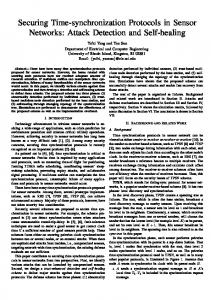
Estimation Error [ppm]

Frequency Error Estimation Accuracy - 95% Confidence Intervals 0.0001

1e-05

Rt

where t A2 g(κ(τ ))dτ is essentially the accumulated error over the A1 interval from tA1 to tA2 . In other words, it computes the average frequency error over the time between the two messages. Thus, assuming that the frequency error changes over time, the error the time synchronization protocol will make in terms of frequency error estimation at the time instance tA2 is δE (tA2 ) = δQ − g(κ(tA2 )),

1e-06

1e-07 10

100 1000 Synchronization Interval [s]

10000

δE f0=32kHz Temperature Limit

Sim f0=1kHz Sim f0=32kHz δE f0=1kHz

Fig. 1. The error in the frequency error estimation of a sensor node is hampered by two different phenomenas: (1) quantization due to the digital nature of a clock, and (2) temperature induced frequency drift. Simulation shows that there is an optimal resynchronization period at which estimation error is minimized.

synchronization accuracy. This increase in resynchronization period reduces the impact of time synchronization on power consumption, as well as communication overhead. II. F REQUENCY E RROR E STIMATION The nominal frequency of a local clock f0 is the fundamental unit of a time synchronization protocol. It is impossible for a system to achieve a better accuracy than 1/f0 due to quantization effects in the local clock. Thus, the local frequency has a major impact in how accurate a time synchronization protocol can estimate its current frequency error. More precisely, δE (T ) =

1 f0 · T

(1)

where δE is the error in the frequency error estimation, and T the resynchronization time between timestamp beacons. Equation 1 suggests that the longer we wait between synchronization exchanges, the better the accuracy of our frequency error estimation. Unfortunately, this is only true in an environment where the temperature doesn’t change. In reality, the frequency error of a clock changes with temperature. Let’s define the temperature dependent frequency as f (t) = (1 + δ(t)) · f0 where δ(t) is the frequency error and can be expressed as δ(t) = g(κ(t)). Here, g() is a function defined by the resonating element, e.g. a quadratic curve for a tuning fork crystal, and κ(t) the temperature at time t. Given two beacons from a remote node A, each containing the precise time the beacons were sent, a node B can estimate its current frequency error relative to node A’s clock using δQ =

(tA2 − tB2 ) − (tA1 − tB1 ) . tA2 − tA1

Without loss of generality, let’s assume that T = tA2 − tA1 and that the clock of node A is perfect. Thus, the measured frequency error becomes T − (tB2 − tB1 ) δQ = = T

R tA2 tA1

g(κ(τ ))dτ T

,

(2)

where δQ is the current drift estimate, and g(κ(tA2 )) the actual drift of the crystal. This gives us the theoretic background to investigate the errors made in frequency error estimation of a time synchronization protocol. In order to verify these results, we need to simulate an actual time synchronization protocol. None of the currently available sensor network simulators capture the effect of change in clock frequency due to changes in environmental temperature. At best, some simulators model different static clock frequency offsets [10], [11], but these offsets are static over the time of a simulation, and are thus not useful for our experiments. We enhanced Castalia [10] with a revised clock model, that takes as input a temperature trace file and adapts the clock’s frequency error at runtime. Since Castalia provides a very good channel and power model for the Texas Instrument CC2420 radio module, we added a realistic timestamping mechanism that models the timestamping errors found on the CC2420 radio chip. In order to evaluate TDTS versus a current time synchronization protocol, we implemented FTSP in Castalia. This implementation is based on the FTSP code currently available in TinyOS 2.1. Verification simulations showed similar accuracies in the simulation of FTSP compared to results found on a real testbed of motes. Figure 1 summarizes the simulated result for two different nominal frequencies, f0 = 1kHz and f0 = 32kHz. It shows that the simulated error of the frequency error estimates follows the two theoretic limits, once limited by the quantization accuracy given by Equation 1, and then hindered by the change of the frequency error over time due to changes in temperature, given by Equation 2. This shows that there is an optimal resynchronization time that minimizes the error in frequency error estimation. This optimum highly depends on the nominal clock frequency f0 , and the temperature environment the node is located at.

III. T EMPERATURE D RIVEN T IME S YNCHRONIZATION The main idea behind TDTS is to measure the temperature during frequency error estimation. Once we learned the relationship between frequency error and temperature (i.e. we found g(κ)), the node can back off and increase the time between synchronization intervals while adapting its frequency error estimation from temperature measurements alone. Thus, the protocol contains two phases: (1) calibration and (2) compensation. It is to note that TDTS itself does not make any assumptions on the network architecture, i.e., it is a technique to elongate the time between resynchronization intervals, and thus is compatible with network synchronization protocols like FTSP, GTSP, or a synchronization tree similar to TPSN or IEEE 1588. However, it is assumed that a node running TDTS, let’s call it slave node, receives accurate time measurements from a remote node, called master, and that the slave node can communicate with its master. This communication is necessary, since the slave node has to let the master node know the resynchronization interval. More detail to this communication will follow in the next two subsections.

3

Average Hourly Beacon Interval of TDTS

Comparison of FTSP and TDTS performance 0.001

40

2000

35 1500

30

1000

25 20

500

15

0

10 0

24

48 72 Simulation Time [h]

Beacon Interval

after 24h

0.0001

FTSP

after 48h

after 60h

1e-05 10 100 Resynchronization Interval T [s]

Temperature

A. Calibration At initialization, the slave node does not know its current frequency error. Thus, it needs to rely on the cooperation of a master node that has knowledge of the accurate time. In order to increase the precision with which the slave estimates its current frequency error, it requests from the master node timestamped beacons with the optimal interval. The slave node can determine this interval by the knowledge of the nominal frequency of the local clock, and some knowledge about the temperature environment it expects, as we explained earlier in Section II. For each timestamp beacon, the slave node notes its current local time time and temperature T. Using this information, and a simple regression on the time, and time offset between the timestamp and local time, the slave node can estimate its current frequency error δQ and offset average offset. It can now store this frequency error in a calibration table containing temperature vs. frequency error estimates. Assuming that the temperature doesn’t change, the slave node can now inform the master that it is calibrated, and thus the master increases the time between beacons. Subsequently, the slave node will switch into the compensation state. B. Compensation During compensation, the slave node regularly measures the environmental temperature. After every measurement, the slave checks the temperature vs. frequency error curve to see if it knows the frequency error for the corresponding temperature. If the table entry is missing, then the node switches back into the calibration state, informing the master to send timestamp beacons at the calibration rate. However, if the frequency error is known then the current frequency error estimate is updated using the calibration information. It is to note that after the update in frequency error, the slave node has to compensate its local offset estimation. More precisely, every time the slave node changes its frequency error estimate after a temperature measurement, it has to update its current local offset estimate using 0 δQ + δQ · (t − t0 ) 2

TDTS w/ calibration

96

Fig. 2. This graph shows the hourly average resynchronization time. In the first 24h, TDTS calibrates the local clock, and thus uses a very short synchronization period. Once calibrated, the resynchronization time rapidly increase and thus saves power and communication overhead.

offset = offset +

Maximum Synchronization Error [s]

45

Temperature [C]

Average Hourly Beacon Interval [s]

2500

(3)

0 where δQ is the old frequency error, δQ the new frequency error, t0 the last local compensation time, and t the current local time.

1000

Fig. 3. If one ignores the one-time calibration overhead, TDTS quickly outperforms FTSP in terms of accuracy with long resynchronization intervals. This is for a 32kHz tuningfork crystal.

Even if the slave node is completely calibrated, i.e., if we found the frequency error estimate for every temperature possible, the master still needs to send the occasional synchronization beacon due to inaccuracies in the calibration. These occasional synchronization beacons assure that the absolute time error between the master and the slave never increases above a certain threshold. After each such beacon, the slave node calculates the absolute time error. If this error is below the required synchronization accuracy, then the slave informs the master to increase the beacon interval, in order to save energy. There are several such increase strategies possible. In our current TDTS implementation, we use an additive increase, multiplicative decrease, similar to TCP’s congestion avoidance algorithm. IV. R ESULTS The difficulty in comparing TDTS to a legacy time synchronization protocol is the lack of a static resynchronization period. The length of the resynchronization period during the calibration phase of TDTS is given by the nominal clock frequency f0 and the expected temperature environment. However, TDTS has its limit. It can not infinitely wait between resynchronization periods and still periodically resynchronizes, as explained in the last section. In addition, TDTS’ average resynchronization period will increase the lesser it has to calibrate. Figure 2 shows the average beacon interval per hour. We can clearly see that during the first 24 hours of the simulation, TDTS is primarily in calibration mode, since it has never encountered the environmental temperatures. However, as soon as TDTS can rely on the calibration information, the average resynchronization period rapidly increases. Compared to FTSP, the overall accuracy of TDTS is very comparable. On average, through the whole 96h simulation, TDTS has an average beacon interval of 329 seconds and 95% of the errors lie within ±4 tics of a 32kHz clock. FTSP with a static resynchronization rate of T = 400 seconds achieves 95% of the errors within ±3.2 tics. However, by examining TDTS after its initial calibration period, TDTS’ average beacon interval increases rapidly, without impacting its overall accuracy. Disregarding the first 24h of the simulation, the average resynchronization period of TDTS increases to T = 439 seconds, after 48h it becomes T = 590 seconds, and after 60 hours even T = 730 seconds. At T = 700s FTSP’s accuracy drops to 95% of the errors within ±11 tics, whereas TDTS maintains the ±4 tics accuracy. Figure 3 illustrates this behavior further.

4

0

28

-20

26

-40

24

-60

22

-80

20

-100

18

-120

16 56 FTSP

58

60

62 64 Time [h]

66

TDTS

68

70

72

Temperature

δQ [ppm]

TDTS Calibration Accuracy 30

Temperature [C]

Synchronization Error [ms]

FTSP vs. TDTS if Synchronization is Stopped 20

1.1e-05 1e-05 9e-06 8e-06 7e-06 6e-06 5e-06 4e-06 3e-06 2e-06 1e-06 0 15

20

25 30 Temperature [C]

TDTS δQ Estimation

35

40

Tuning Fork Model

Fig. 4. Illustration of what happens if time synchronization is stopped. We can clearly see how FTSP’s performance worsens once the temperature starts to change, whereas TDTS keeps the synchronization accuracy at a much higher level.

Fig. 5. TDTS estimates the frequency drift function g(κ) for the current temperature, and stores it in a calibration table. In our simulation, g(κ) is a quadratic curve, as found in the tuningfork crystals. Even with only a 0.25C temperature resolution, the performance of TDTS is extremely high.

A. Robustness

insight into time synchronization by solving a problem introduced by the underlying hardware a synchronization protocol relies on.

One further advantage of TDTS over a legacy time synchronization protocol is in scenarios where communication either gets lost or severely impacted. Examples of such scenarios are heavy environmental conditions (snow on antenna, heavy rain, etc.), mobility (moving outside radio range of peers), or covert military operations where radio silence is crucial. In these scenarios, TDTS switches automatically into a TCXO mode, where the frequency of the local clock gets regularly updated. In contrast, legacy synchronization protocols will have to rely on the last frequency error measured. Figure 4 compares the synchronization accuracy of TDTS with FTSP if the synchronization process gets stopped after 56 hours. As soon as the temperature starts to change significantly from the last temperature observed during the last synchronization interval, FTSP starts to loose accuracy, while TDTS can keep its accuracy at a very precise level. Over the 16 hours where no resynchronization occurs, TDTS accumulates only 4ms of time synchronization error. This corresponds to a clock stability of < 0.07ppm! Figure 5 shows the calibration information TDTS collected during this experiment, and compares it to the actual clock model fed into the simulator itself. This plot shows that a time synchronization protocol can successfully temperature calibrate a local clock oscillator, and thus removes the factory calibration step necessary for a TCXO. V. C ONCLUSION Temperature Driven Time Synchronization is a first step towards an automatic temperature calibration of a local clock. We showed that TDTS can outperform a standard time synchronization protocol by exploiting temperature information to increase the synchronization intervals. This increase results in overall network power savings, since fewer synchronization messages have to be transmitted. In addition, TDTS improves the robustness of an embedded device in case of communication difficulties. This paper introduces a first implementation of TDTS. For this implementation, we chose FTSP as the host synchronization protocol, since it is one of the most widely used synchronization protocols in the sensor network community, and its implementation is readily available. However, we plan to push this research further, improving on some of FTSP’s problems by cherry-picking specific attributes of other time synchronization protocols, like the local synchronization accuracy of GTSP or the removal of propagation delay and send/receive latencies of TPSN. Overall, we believe that this work gives new

ACKNOWLEDGMENT This material is supported in part by the U.S. ARL and the U.K. MOD under Agreement Number W911NF-06-3-0001, by the NSF under award CNS-0614853, and by the Center for Embedded Networked Sensing at UCLA. Any opinions, findings and conclusions or recommendations expressed in this material are those of the authors and do not necessarily reflect the views of the listed funding agencies. The U.S. and U.K. Governments are authorized to reproduce and distribute reprints for Government purposes notwithstanding any copyright notation herein. R EFERENCES [1] J. Elson, L. Girod, and D. Estrin, “Fine-grained network time synchronization using reference broadcasts,” ACM SIGOPS, vol. 36, pp. 147– 163, 2002. [2] S. Ganeriwal, R. Kumar, and M. Srivastava, “Timing-sync protocol for sensor networks,” SenSys, 2003. [3] J. Eidson, Measurement, Control, and Communication Using IEEE 1588. Springer, 2006. [4] T. Cooklev, J. Eidson, and A. Pakdaman, “An implementation of IEEE 1588 over IEEE 802.11 b for synchronization of wireless local area network nodes,” IEEE Transactions on Instrumentation and Measurement, vol. 56, no. 5, pp. 1632–1639, 2007. ´ L´edeczi, “The flooding time [5] M. Mar´oti, B. Kusy, G. Simon, and A. synchronization protocol,” SenSys, pp. 39–49, 2004. [6] P. Sommer and R. Wattenhofer, “Gradient clock synchronization in wireless sensor networks,” in IPSN, 2009. [7] T. Schmid, R. Shea, Z. Charbiwala, J. Friedman, Y. H. Cho, and M. B. Srivastava, “On the interaction of clocks, power, and synchronization in embedded sensor nodes,” under submission, 2009. [8] S. Ganeriwal, D. Ganesan, H. Shim, V. Tsiatsis, and M. B. Srivastava, “Estimating clock uncertainty for efficient duty-cycling in sensor networks,” in SenSys, pp. 130–141, 2005. [9] W. Zhou, H. Zhou, Z. Xuan, and W. Zhang, “Comparison among precision temperature compensated crystal oscillators,” Frequency Control Symposium and Exposition, 2005. [10] A. Boulis, “Castalia: revealing pitfalls in designing distributed algorithms in wsn,” in SenSys 2007. [11] M. Varshney, D. Xu, M. Srivastava, and R. Bagrodia, “sQualNet: A scalable simulation and emulation environment for sensor networks,” IPSN, 2007. [12] R. Musaloiu-E, C. M. Liang, and A. Terzis, “Koala: Ultra-low power data retrieval in wireless sensor networks,” IPSN, 2008.