16th European Signal Processing Conference (EUSIPCO 2008), Lausanne, Switzerland, August 25-29, 2008, copyright by EURASIP
TEMPERATURE FIELD MODELING AND SIMULATION OF WIRELESS SENSOR NETWORK BEHAVIOR DURING A SPREADING WILDFIRE Elias S. Manolakos1,
Dimitrios V. Manatakis1 and Gavriil Xanthopoulos2
1
Department of Informatics and Telecommunications, University of Athens Panepisitmiopolis, Ilisia, 15784, Athens, Greece phone: + (30)-210-7275312, email:
[email protected] 2
National Agricultural Research Foundation (N. AG. RE. F.), Aigialias 19 & Halepa, 15125, Athens. Greece
ABSTRACT We present the development of a simulator that approximates the behaviour of a wireless network of temperature sensors deployed in the area affected by a wildfire. It is based on a novel signal processing approach in which the temperature experienced at a sensor due to a spreading fire front is modelled as the mixture of two-dimensional Gaussian distributions. We present the justification, development and validation of the proposed model. Our work enables the in-silico generation of synthetic, yet realistic, sensor temperature data sets. Due to the lack of real data, such data sets can be useful in deriving optimal sensor network deployment strategies for fire detection and progress monitoring in a specific area, under different scenarios for the expected wind conditions, and for calibrating fire spread prediction models. 1.
INTRODUCTION
During the last few years, significant advances in embedded hardware and software technologies are driving down rapidly the cost of wireless sensor networks (WSN) and allow largescale WSN deployments for environmental monitoring applications to become viable. There exist already several ongoing WSN projects in Europe and worldwide for assessing habitat changes, monitoring the evolution or predicting the risk of catastrophic phenomena such as floods [1], fires [2], earthquakes. volcano eruptions, etc. Modeling wildfire behavior is a very difficult problem due to, among other reasons, the large number of timevarying parameters governing this complex phenomenon. However, since it is a very useful tool for fire management, significant efforts have been devoted over the last decade to the development of fire behavior prediction models [3], [4]. In most cases, models have been designed to simulate fire spread, linear intensity and flame length but not temperature. In few cases, especially for modeling crown fire initiation, certain modelers have proposed sound algorithms to predict, for example, the time-to-temperature profiles above a spreading flame front [5]. Since low cost digital temperature sensors (that can measure usually up to ~120 oC) have become commodity items it becomes feasible to deploy WSN based systems for distributed fire detection and monitoring. Such a system can contribute to the on time fire detection via intelligent distrib-
uted signal processing and data fusion algorithms and also help us calibrate periodically models used to predict the evolution of a fire front under different prevailing wind conditions in the affected region. These capabilities can be particularly important in the so called Wildland Urban Interface (WUI) regions surrounding our modern cities where the catastrophic impact of a rapidly spreading fire can be tremendous to human lives and property, as we have recently experienced in Athens, Greece, Los Angeles, USA etc. Fire spread modelling is a very challenging problem since it depends on many factors, such as ground morphology, combustion fuel, moisture and most importantly on the wind speed and direction which may be changing rapidly. Nevertheless, there exist several software tools (such as FARSITE [6], FSE [7] etc.) that consider a geographical region of interest as a grid of “cells” and use algorithms to predict for every cell the time of a fire arrival. They are almost all based on the ground breaking work of Rothermel [8] which given the type of fuel and the wind conditions can estimate several local fire related properties, such as the flame length, fire intensity, etc for each cell of an evolving fire front. We have developed and present here a WSN simulator that complements traditional fire spread modelling in the following sense. It takes as input the current fire front positions (i.e. the centers of the fire front “cells”) estimated by an existing fire spread software program (in our case the FSE, developed by Technoma S.A.[7]) and produces as output, by using signal processing techniques, the expected temperature vs. time curves at specified sensor locations. The operation of the simulator is based on a new modelling approach with two novel elements: (a) The temperature field induced locally by each fire front cell is assumed to be 2D Gaussian with a full covariance matrix, which is updated in every simulation step based on the current flame and prevailing wind conditions at the cell, and (b) the temperature value experienced at a sensor location is modelled as a mixture of K (a small integer) 2D Gaussian local temperature field models, one Gaussian model for each one of the K closest fire front positions to the specific sensor, where distances are measured in the Mahalanobis sense. To the best of our knowledge, our WSN simulator is the first of its kind in that it provides the ability to generate in silico synthetic temperature field data sets under different fire scenarios (e.g. different rates of spread, wind speed and directions etc) and different distributed sensor node deploy-
16th European Signal Processing Conference (EUSIPCO 2008), Lausanne, Switzerland, August 25-29, 2008, copyright by EURASIP
ments. With this tool we can place virtual sensors at any desirable location in a region of interest, initiate a fire hazard with certain properties and study how fire propagation speed, fire intensity, wind speed and direction etc. are expected to affect the temperature field i.e. the spatio-temporal distribution of temperatures induced by the spreading fire front at sensor locations. Due to the scarceness of WSN based data sets from real fires, such synthetic data sets are very useful in evaluating different WSN deployment strategies for detection and progress monitoring purposes. Furthermore, if a WSN of temperature sensors is really deployed in a field, it becomes possible to calibrate fire front location predictions (produced by the FSE, FARSITE etc) by correlating periodically real field sensor measurements with those predicted by the simulator. Our work is part of the activities carried out within the framework of the SCIER project [9], co-funded by the European Commission under the 6th framework of R+TD. The rest of the paper is organized as follows: In Section 2 we present the justification for using Gaussians to model the distance-temperature relationship and discuss the methods used to estimate the model parameters and sensor temperatures. The simulator developed is presented in Section 3. Model validation results are presented in Section 4. Finally our findings are summarized and work in progress is outlined in Section 5. 2.
TEMPERATURE FIELD MODELLING
2.1 Model justification The first challenge for the development of our simulator was how to model the temperature field that is induced locally under specific wind conditions (speed and direction) by a flame with specific site characteristics (length or height). One of the difficulties we had to face was that there is little published work on the relation of temperature to distance (from flame). Most scientists who study fire behaviour are concentrating on heat flux (kW/m2) instead of temperature because the physics of the phenomena related to the different phases of a fire (ignition to extinction) are better explained in terms of the heat flux. However, sensors measuring heat flux are not preferred for WSN applications because they are expensive (relatively to commodity digital temperature/humidity sensors) and quite sensitive to mechanical stress. Furthermore, for the range of temperatures that the commodity sensors can measure (i.e. up to 120 oC) it is reasonable to assume a linear relationship between temperature and heat flux measurements as it can be verified from the experimental results reported in [10] and [11]. For short flames produced by surface fires and intermediate crown fires (with flame height less than 8m) the work in [12] provides a relationship between temperature, distance from flame and flame length. The equations which are used are the following: (1) I = 3 0 0 ⋅ L2 −I Q = 6 0 1 − e x p 300 ⋅ D
(2)
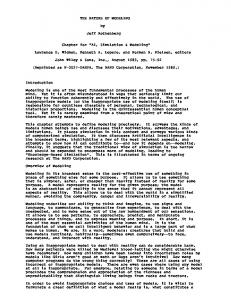
Figure 1 - 1D Gaussian models can capture the temperature - distance relationship for fires of both small and large flame size fires. The larger the flame size of the modelled fire the larger the variance.
where I, L, Q and D denote fire intensity (in kW/m), flame length (in meters), radiation intensity (in kW/m2) and the distance from the flame position (in meters) respectively. Assuming a linear T = a Q relationship (with a=10 as inferred from [10] and [11]) we can establish a temperature – distance T = fL (D) relationship for any given L. On the other hand for large flame height, the authors in [13] have presented a model that estimates the net radiant energy transfer to a fire fighter standing at a specified distance D from a fire of a height L. It is observed that the larger the flame height the larger is the distance from the flame that would result to a specific heat flux (and sensed temperature) value. We can use this work to extract a T = gL (D) relationship for large flame heights, L > 8m. It is interesting that the two different methods, for small [12] and large [13] flame sizes, produce approximately the same temperature estimates at the cutoff point of L=8m. We will show next that both functions fL (D) (for smaller flames) and gL (D) (for larger flames) can be approximated quite well using 1D Gaussians. 2.2. 1D Gaussian temperature-distance models Let us consider now a set of normalized one dimensional (1D) zero-mean normal distribution curves with different variance (Figure 1) and assume that each one of them models the temperature vs. distance behaviour of a specific fire. The outer (inner) curve corresponds to the fire with the larger (smaller) flame height. Observe that as the flame height increases, temperatures in our region of interest (say 50-150 o C) are sensed from greater distances from the flame (assumed to be located at the origin) which agrees with our intuition and the models described in [12] and [13] for both small and large fires. Furthermore, the normal distribution can capture the fact that although a small fire is sensed at a smaller distance, it causes a more abrupt temperature change once it comes within sensing range. Using the empirical model proposed in the literature for small and large flame lengths [12], [13] we can extract for every fire size parameter L a training set with N distancetemperature data points {x(i), t(i) , i =1,2...N} and use it to compute the Maximum Likelihood Estimate (MLE) of the standard deviation σMLx of the zero-mean 1D normal distribution model that fits best to the particular data set. To esti-
16th European Signal Processing Conference (EUSIPCO 2008), Lausanne, Switzerland, August 25-29, 2008, copyright by EURASIP
mate the maximum temperature value Tmax of the model 2 N (0, σ MLx ) derived for each L we can use the same train-
ing set and compute first Tmax(i) using Equation (3): x (i ) 2 (3) t ( i ) = T m ax ( i ) ⋅ ex p 2 2σ M L x Then Tmax can be estimated by averaging the Tmax(i) values: (4) 1 N t (i ) Tm ax = ∑ 2 N i =1 x (i ) exp 2 2σ M L x In practice, using only N=3 data points and specifically the distance-temperature points at temperatures {t(i)= 50, 70, 100} degrees Celsius in the range of interest and we can achieve a very good least squares fit of the 1D Gaussian model to the data sets for both small-size and large-size fires. The root mean square error (RMSE) of the fit for the values L={1m, 3m, 5m, 10m, 20m, 30m} is small and specifically, RMSE={0.95, 0, 0, 6.87, 6.77, 7.61} degrees Celsius respectively. 2.3 2D Gaussian modelling of temperature-distance For simulating the temperature field induced locally by a fire of flame size L, we need to move from the 1D to a 2D zero mean normal distribution model i.e. we need to estimate the diagonal covariance matrix, σ M2 L x Σd = 0
0
σ M2 L y
where σMLx has already been estimated. However, for the ellipsoids that correspond to the iso-temperature curves it holds that:
R=
M ajo r ax is o f the ellip se σ M L x = M ino r axis o f the ellip se σ M L y
(5)
thus we could estimate σMLy if we knew the ratio R of its principal axes. This can be accomplished, however, based on Anderson’s work [14] which suggests that given the wind speed it is possible to estimate the shape of the ellipsoid that approximates the affected area and also provides a method for computing the ratio of its principal axes. The burned area shape in the initial fire stages, has immediate relation with heat radiation [15] and thus with temperature. So it is logical to assume that the temperature field induced locally by a fire front can also be modeled by an ellipsoid with isotemperature curves exhibiting the same principal axis ratio as the ellipsoid that approximates the affected area. This provides an additional justification for using 2D Gaussian models for the local temperature field. So having R and σMLx we can now use Equation (5) and find σMLy. Furthermore, using the prevailing wind direction θ (relatively to the principal horizontal x-axis) which is assumed to be known for every cell of the front, we can rotate the covariance matrix so that the ellipsoid principal axis is now aligned with θ, giving rise to a zero-mean, full covariance matrix (Σ) temperaturedistance 2D Gaussian model (see Figure 2).
Figure 2 - The temperature field induce locally by each fire front point is modeled as a 2D Gaussian whose time-varying parameters depend on the flame size, wind speed and wind direction.
In summary, to estimate the 2D Gaussian temperature field induced locally by a fire front cell at time t, we need the following information: • The fire front cell center coordinates. • An estimate of the size of the flame L, i.e. the flame height, or the flame length and the angle φ of the flame with the horizontal level. This is needed to estimate σMLx at time t. • The prevailing wind parameters i.e. the wind speed and direction, used to estimate the ratio R, and then σMLy and the full covariance matrix Σ. In practice, the wind related information can be obtained either by dedicated distributed wind sensors deployed in the area to be protected, or by meteorological stations in the same general region. The fire front characteristics (i.e. cell coordinates, flame size) are estimated periodically by a fire spread prediction program. So our temperature field modeling (TFM) can be thought as an operation (and software component) evoked at the end of each iteration (time step) of a fire spread simulation component which generates predictions for the new fire front locations and flame characteristics, using area specific static information (i.e. fuel model, moisture content etc) and dynamic information (wind speed and direction). 2.4
Sensor Temperature Estimation Algorithm
Having available the minimal set of parameters listed before at time t, we can generate the temperature field induced by a fire front and calculate the expected temperatures at any specified virtual sensor position. We model the process that generates the temperature at a sensor as a mixture of K 2D normal distribution components, that is, one component for each one of the K fire front points that are “nearest” to the sensor under consideration. Distances are measured in the Mahalanobis sense, to account for the potentially different wind and flame characteristics leading to potentially different full covariance matrices for each fire front cell at time step t (see Figure 2). The algorithm used is summarized below: For each Sensor node s and time step t:
16th European Signal Processing Conference (EUSIPCO 2008), Lausanne, Switzerland, August 25-29, 2008, copyright by EURASIP
1. Find the K “nearest” fire front points to sensor s, i.e. those that have the smallest Mahalanobis distance,
(
d1…dK, where d j = x j − x s
T
)
Σ −j 1 ( x j − x s ) j=1… K
2. For each fire front point j=1,2…, K use the corresponding 2D Gaussian model and compute: 1 1 j=1… K ⋅ exp − d j gj = 2π Σ j 2 Calculate weights wj…wK using wj = gj/G where
∑
k
w j = 1 and G = ∑ j =1 g j k
j =1
3. Estimate the expected sensor s temperature using K 1 ts = Tmax ⋅ ∑ w j ⋅ exp − d j 2 j =1
where Tm ax = max {Tm ax ( j )} j ∈[1... K ]
3. TEMPERATURE FIELD SIMULATION
Our temperature field simulator (TFS) assumes the existence of a fire spread engine that simulates fire front progression. For example, the Fire Spread Engine (FSE) developed by Technoma S.A [7] takes as input static parameters, such as ground morphology, combustion fuel, moisture, and dynamic parameters such as wind speed and direction, ignition points etc. and estimates the time of fire arrival at every affected cell. Moreover, the FSE can provide the fire intensity, flame length and heat energy at each cell of the fire front. Our TFS software component uses as input: the fire front condition information (e.g. as produced by an FSE) , the assumed virtual sensor locations and the value of parameter K (the number of close by cells assumed to affect a sensor). It generates the estimated temperatures at sensor locations as a function of simulation time t, It also allows us to visualize: • A temperature field snapshot at every time step t as simulation progresses (temperature images). • For all sensors the temperature vs. time steps “heat map” at the end of the simulation. • Temperature vs. time curves for selected sensors. Figure 3 shows a snapshot of our WSN simulator user interface. The simulation parameters are entered on the left. The top map shows the area affected by the fire (yellow) and the deployed sensor locations (crosses). Sensors are colored according to their temperature at the current simulation time step. The bottom map shows the corresponding “temperature image” at the current simulation time (t=116 min.). Each pixel corresponds to a virtual sensor and its color represents the current sensor temperature value, based on the color bar shown on the right. It is also possible to run temperature field simulations without using afire spread software. In this case our program simulates crudely fire spread scenarios under the assumption that the fire affected area is approximated by an ellipse whose shape is determined by the wind speed and direction [14].
Figure 3 - Simulation snapshot at time t=116min after fire detection. See text for details.
The ellipse center is moving at a fixed speed (Rate Of Spread-ROS) along the fixed principal axis direction and the ellipse size is changing with time. The spread across the minor axis is progressing at a rate b*ROS, where 0