... net transport of water due to the wind stress with the transport directed 90 degrees ..... analysis was performed on the temperature and wind data. A perfect or ...
AN ABSTRACT OF THE THESIS OF
Robert Hathaway Bourke (Name)
in
Oceanography (Major)
for the
M. S.
(Degree)
presented on 7-A'Jt4191'8 (Date)
Title: MONITORING COASTAL UPWELLING BY MEASURING ITS EFFECTS WITHIN AN ESTUARY
Abstract approved:
Redacted for Privacy
Robert L. Smith
Temperature, salinity, and dissolved oxygen concentration measured in an estuary were analyzed to determine if the effects of coastal upwelling could be observed and used to effectively monitor the degree of upwelling.
Hydrographic data collected weekly at a point four miles from the entrance of Yaquina Bay (Buoy 15) were analyzed for their appli-.
cability as indicators of coastal upwelling. Only data collected during the known upwelling season off Oregon of May through October were
considered. Low temperature, low dissolved oxygen concentration,
and high salinity occurred when the wind was strongly from the north-conditions expected during times of active upwelling.
A regression analysis was performed to establish the relationship between water temperature and wind velocity averaged Over a three day period. The two were significantly related. Various weighting
schemes were applied to the wind observations to obtain an average
wind which would provide the best correlation between wind and
temperature. A wind averaged over four days and weighted heaviest during the third 24 hour period prior to the temperature observation
resulted in the best correlation. A prediction model was formulated to allow for the prediction of
water temperature 24 hours in advance based upon the known wind field during times of active upwelling.
Comparisons of temperature and salinity from five miles off the coast with that in the estuary established that the upwelled water entering the estuary on the flood tide originated from a depth of about
20 meters at three-five miles off the coast. Measuring the temperature, salinity, and oxygen concentration of the bottom water near the mouth of an estuary does provide an
effective, reliable, and simple method of monitoring the stage of upwelling occurring outside the estuary.
Monitoring Coastal Upwelling by Measuring Its Effects Within An Estuary Robert Hathaway Bourke
A THESIS
submitted to
Oregon State University
in partial fulfillment of the requirements for the degree of Master of Science June 1969
APPROVED:
Redacted for Privacy
Assistant Professor of Oceanography In Charge of Major
Redacted for Privacy
Chair\iian of Departme4t of Oceanography
Redacted for Privacy
Dean of Graduate School
Date thesis is presented
7_44E 19'8
Typed by Marcia Ten Eyck for Robert Hathaway Bourke
ACKNOWLEDGEMENTS
I wish to express my deep appreciation to Dr. Robert Smith, who
served as my major professor, for suggesting this study and for contributing his time and efforts so generously to this project. I am deeply indebted to Dr. Fred Ramsey, who devoted much
valuable time and effort while serving as statistical consultant. His
help with the statistical analysis is greatly appreciated. I wish to thank Mr. Lynn Scheurman for his assistance in programming.
I wish to extend my gratitude to Dr. Herbert Frolander who generously allowed me the use of his data collected from the Yaquina estuary. I am especially grateful to all those un-named biological
oceanographers who, for the past eight years, have made weekly
trips to Newport to collect the data used in this report. I also want to thank Mr. Dana Kester for his editorial comments, for his help with the oxygen analysis, and for serving as my 'TDevil's Advocate.
Lastly, to my wife, Portia, I owe a special thank you. Her encouragement, under standing, and companionship are gratefully acknowledged.
TABLE OF CONTENTS
Page INTRODUCTION
Review of Upwelling Indicators Purpose of Study ESTUARIES
Definition
Classification The Yaquina Estuary
DATA COLLECTION
Procedure DATA ANALYSIS
Hydrographic Data Tidal Analysis Wind Analysis Dissolved Oxygen Summary STATISTICAL ANALYSIS
General Considerations Components of the Wind Regression Procedure
Weighted Wind Averages Results of Weighting Confidence Interval
Prediction Limits Discussion
OTHER OBSERVATIONS
Origin of Upwelled Water Upwelling Cycles SUMMARY AND CONCLUSIONS
1
1
2 2 5 5 5 7
9
9
ii ii
12 13 17 is
21 21 22 23 27
28 31 32 35 38 38
44 47
TABLE OF CONTENTS Continued
Page BIBLIOGRAPHY
50
APPENDIX I
List of Symbols
53
LIST OF TABLES
Page
Table I
Weighting schemes attempted.
27
II
Weighting schemes indicating the importance of weighting the third day preceding the temperature observation.
29
Weighting schemes wherein the first two days preceding the temperature observation are weighted heavier.
29
IV
Weighting schemes indicating the relative unimportance of the fourth day.
29
V
Various combinations of weighting schemes.
29
VI
Weighting schemes for prediction with resultant variance.
32
III
LIST OF FIGURES
Page
Figure 1
Bathymetry of Yaquina Bay.
8
2
Temperature and salinity at Buoy 15 measured over 27 hour period, 9-10 August 1963.
14
3
Temperature and salinity at Buoy 21 measured over 25 hour period, 11-12 September 1966.
15
4
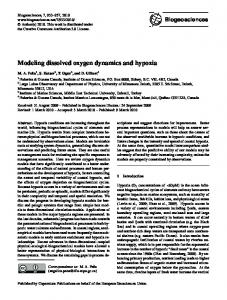
Plot of temperature, salinity, percent oxygen saturation, and north-south component of wind velocity measured at Buoy 15 during the summer months 1965-1967.
19
S
Graph of water temperature at Buoy 15 versus north-south component of wind velocity.
24
6
Regression analysis of temperature on wind velocity.
36
7
T-S diagrams for NH-5, Buoy 15 and Otter Rock.
39
8
9
Temperature and salinity comparisons at Otter
Rock and Buoy 15 for 1961-1963.
Average monthly temperature and salinity for period 1960-1967.
43
45
MONITORING COASTAL UPWELLING BY MEASURING ITS EFFECTS WITHIN AN ESTUARY INTRODUCTION
Review of Upwelling
Upwelling may be defined as the ascending movement of subsur-
face water into the surface layer in response to the offshore transport of surface water. It is a phenomena known to occur off the Oregon coast during the summer months and has been studied exten-
sively by several authors. The chemical properties of upwelling
were discussed by Park, Pattullo, and Wyatt nutrients (Matson, Hebard,
1966)
1964)
(1962);
its effect on
and plankton distribution (Cross,
have been investigated. Smith
model for coastal upwelling, and Collins
(1964)
(1964)
1964;
developed a
discussed the effects
of upwelling on the permanent oceanic front off the Oregon coast.
The offshore transport during the early stages of upwelling has been computed by Smith, Pattullo, and Lane
(1966).
At this time coastal
upwelling is being investigated by the use of self recording current
meters and thermographs as a continuing research effort by the Department of Oceanography at Oregon State University.
Ekman's classic paper of
1905
(Ekman,
1905)
provided the basis
for the physical explanation of upwelling and the effects of wind
stress on the sea surface. His results provide for a net transport of water due to the wind stress with the transport directed
90
degrees
2
to the right (left) of the wind direction in the Northern Hemisphere (Southern Hemisphere).
The northerly winds, which predominate
during the summer months off the Oregon coast, transport water
offshore and necessitate a rise of deeper water near the coast. This water generally comes from depths not exceeding 200 meters
(Sverdrup et al., l94). Indicators
Because the upwelling process brings subsurface water into the
surface layer, anomalies will normally result in the distribution of physical and chemical properties. These anomalies can be used
as indicators of upwelling (Park, Pattullo, and Wyatt, 1962). Up-
welled water is generally identified by its colder temperature, low oxygen content, and higher salinity when compared to the surround-
ing water or when compared to the same waters in times when upwelling is not active. Other indicators of upwelled water would be
increased alkalinity, inorganic phosphate, and hydrogen ion concentration. Purpose of Study
Although coastal upwelling has been rather extensively studied, few investigations have been made of the effects of upwelling on
estuaries. Pearson and Holt (1960) have reported their findings of
3
low oxygen concentration values in Grays Harbor, Washington. They conclusively proved that the low dissolved oxygen concentra-
tions, which were originally attributed to industrial pollution, were actually a consequence of oxygen-poor upwelled water entering on the flood tide.
The effect of upwelling on the biological population,
notably zooplankton, within an estuary was observed by Frolander
He related the distribution of several species of zooplank-
(1964).
ton found in Yaquina Bay, Oregon, to various temperature and salinity zones.
The population of the several species fluctuated as
the environment changed. Although tidal variations were largely
responsible for these fluctuations, the changes in temperature and salinity caused by the variability in the strength of upwelling were large enough to exert a strong influence on the population. However, a detailed study of the physical and chemical effects of coastal upwelling on an estuary has not been undertaken. It is
the purpose of this paper to investigate or determine for the Yaquina estuary: 1)
if coastal upwelling can be adequately observed and monitored within an estuary,
2) assuming upwelling can be monitored within an estuary,
the correlation between wind velocity and water tern-
perature in order to obtain a prediction equation for
water temperature,
4
3) the length of the upwelling season, " i. e., its onset
in spring and cessation in fall,
4) the mean values of temperature, salinity, and dissolved oxygen concentration that can be expected for each month of the "season.
In order to establish part one, which is the heart of the thesis, it will be necessary to establish that a relationship exists between estuarine water and oceanic water. It will be shown, in fact, that
the water in the bay sampled at high tide is coastal oceanic water, uninfluenced by estuarine processes. Furthermore, it will be shown that within the estuary the usual indicators of upwelling
respond to the winds in the same manner as has been established for known coastal upwelling regions.
5
ESTUARIES
Definition
An estuary as defined by Pritchard (1952) is "a semi-enclosed coastal body of water having a free connection with the open sea and
containing a measurable quantity of sea salt. " This broad definition
lends to subdivision of estuaries into several types based on various factors. Pritchard classified estuaries into two major types based on fresh water addition and evaporation.
The "negative" estuary
is one in which evaporation exceeds precipitation. A "positive" estuary exists when the fresh water input exceeds the evaporation.
Pritchard further classified estuaries according to their geomorphology.
The Yaquina estuary is classified as a "coastal plain"
estuary.
These are drowned river valleys and are generally posi-
tive although they may change to negative if stream flow is decreased
or diverted, or evaporation increases. All Oregon estuaries may be classified as positive coastal plain estuaries. Clas sification
Pritchard (1955) has subdivided positive coastal plain estuaries
into four types, A, B, C, and D, based upon the observed circulation patterns and salinity distribution. Using this classification system, Burt and McAlister (1959) have identified the major Oregon
estuaries including the Yaquina estuary based upon the measured salinity difference between surface and bottom water at high tide at
the point where the water is half salt and half fresh.
The Type A estuary is a two layered or stratified estuary in which the salinity difference from surface to bottom is
200/00
or
greater. This type of estuary requires a low tidal range, a large depth to width ratio, and a high river runoff. This estuarine system is not found in Oregon although the Umpqua estuary approaches it during extended periods of high runoff.
The Type B estuary is one that is partly mixed with a salinity difference ranging from 4°/oo to 19°/oo.
The partly mixed estuary
is very common in Oregon and is usually present during times of high river runoff.
The Type D or well mixed estuary has a salinity difference of 3°/oo or less. High tidal ranges to provide energy for mixing, low
river runoff, and wide shallow topography are conditions which
create the well mixed estuary. In Oregon many of the estuaries are of this type and change to Type B only during the time of the spring runoff.
Pritchards Type C estuary is not found in Oregon (Burt and McAlister, 1959).
7
The Yaguina Estuary
Due to the relatively high tidal range in Yaquina Bay of about 5. 5 feet, the low river runoff, and the small depth to width ratio
of the estuary, a well developed two layered system seldom, if
ever, exists. In the winter and spring when runoff is high, the estuary generally becomes partly mixed (Type B).
Throughout the
summer months and into the fall (the period covered by this report) the estuary was always well mixed (Type D). At high tide the salinity
difference rarely exceeded to 0. 3
0
10/00
and generally ranged from 0.
00/00
/00.
According to a survey made by the U. S. Coast and Geodetic Survey in September and October of 1955 when the estuary was well
mixed, tidal current velocities near the entrance were found to be in excess of two knots (Kuim and Byrne, 1966). At all depths the maxi-
mum ebb current velocity was slightly greater than that of the flood. At Buoy 15, approximately four miles upstream from the entrance, tidal current velocities were reduced to about one knot. Yaquina Bay (Figure 1), is a body of water about 4. 5 square
miles in area with a major channel, two large tidal flats, and numerous sloughs. The channel is dredged to a depth of 26 feet
from the bar at the entrance to the turning basin opposite McLean Point. From this point upstream to Toledo the channel depth is
maintained at 12 feet.
I24 00'
NEWPORT McLEAN
OBSERVATION
POINT
RID6.)
0
PORTLAND
C"
YAQULNA BAY
TOWER
SOUTUBE&CH
'
B - 15
0 44
36'
COQUILLE POINT
COOS RAY
OREGON
YAOUINA
N
B-21
8-3
ONE6TTA NAUTICAL MILES
ERI
POINT
9fi
STATUTE MILES
Figure 1. Bathymetry of Yaquina Bay. Indicated also are the sampling stations at Buoys 15, 21, 29 and 39. Source: K'ulrri and Byrne, 1966.
DATA COLLECTION
Procedure Since early in
1960
hydrographic and biological sampling have
been undertaken on a weekly basis at selected stations in Yaquina Bay and River (Frolander,
1960-1967).
The sampling has been per-
formed from a small boat by students in biological oceanography at Oregon State University. Sampling has been done primarily at four
mid-channel stations -- Buoys 15, 21,
29,
and 39; occasionally
stations were made off the Marine Science Center (Buoys 8 or 9) and under the Yaquina Bay bridge.
Figure 1 shows the location of
the sampling stations and the approximate water depth at each station.
Surface samples were collected for salinity and dissolved oxygen determination; surface temperatures were determined using a bucket thermometer. To obtain bottom samples a Nansen bottle
with one reversing thermometer was lowered to within a meter of the bottom.
Upon retrieving the cast, the temperature was read
and the samples were drawn for salinity and dissolved oxygen analyses. The oxygen samples were then immediately pickled' with manganous sulphate reagent and alkaline iodide solution.
The concentrated sulphuric acid was not added until several hours later when the oxygen analysis was performed at the Oceanography
10
Building on the Oregon State University campus in Corvallis, using the modified Winkler method (Strickland and Parsons, 1965).
The salinity of the water was measured by personnel at the Marine Science Center in Newport using an inductive salinometer.
Prior to January 1963, salinity was determined by titration with
silver nitrate. Upon completion of the hydrographic sampling phase at each
station, plankton samples were collected by towing two ClarkBumpus samplers utilizing number 6 and 12 mesh nets and then towing a half-meter net. All tows were generally upstream at
bottom, mid-depth and surface levels. No attempt will be made in this paper to correlate the physical and biological oceanographic data.
11
DATA ANALYSIS
Hydrographic Data
As indicated in the previous section, temperature, salinity, and dissolved oxygen concentration were measured weekly throughout
the year at four stations in the Yaquina estuary. Upwelling off the Oregon coast is known to occur during the summer months. A perusal of the data led to the conclusion that only data from the months of May through October were necessary in order to encompass the upwelling seasOn.
Measurements were made at the surface and
about one meter from the bottom at each station. In order to observe the oceanic effects within the estuary only the bottom measurements were evaluated.
This minimized the external influences of heating
by solar radiation and dilution by river runoff and precipitation. Although the effects of dilution were small for most of the six month
periods under consideration, the effects of heating could be quite noticeable. For example, at high water the surface temperature
at Buoy 15 was usually about one degree centigrade warmer than the bottom water; at low tide this difference could amount to four degrees.
Because the water depth in the estuary was so shallow at low
tide (five to six meters at Buoys 15 and 21; two to three meters at Buoys 29 and 39), the water was subject to extreme fluctuations in
12
temperature and salinity between high and low tide. At Buoy 15, for
instance, the water temperature would increase from 8 to
90
C at
high tide to 13-14° C at low tide. Salinity changes between high and low tide were about 20/00 near the estuary entrance and about 40/00 above Buoy 29. It was obvious, therefore, that only measurements
made at high tide would lead to a valid interpretation of oceanic conditions.
Tidal Analysis
Because no attempt was made to synchronize the time of sampling with the tides, it was necessary to determine which obser-
vations were made during periods of high tide. Establishing that an observation was taken during the time of high water proved to be somewhat subjective. The time of each observation was compared
with the predicted time of high tide from the Tide Tables of the U. S. Coast and Geodetic Survey (U. S. C. and G. S., 1960-1967).
The
predicted high water time used was that computed for the town of Yaquina, this being the closest point to Buoy 15.
Neal (1966) in a
paper on tidal currents in Yaquina Bay, stated that the predicted
times were generally good, although nearly all were earlier than the observed tide by 30 minutes or less. In August 1963 at Buoy 15 and in September 1966 at Buoy 21 observations were made every hour for a period of 27 and 24 hours, respectively. The observed
13
temperature and salinity were plotted and the predicted time of the tide indicated (Figures 2 and 3). In each case the predicted high
tide occurred earlier than the observed high tide in concurrence with Neal's conclusions. Based on the temperature curve the
duration of the high tide was approximately three hours; this was
the length of time that the temperature remained at a minimum. In
order to include as many observations as possible, the high tide "window,
or duration time, was determined to be one-half hour
prior to the time of the predicted high tide and two hours after it; observations falling within this two and one-half hour window were
included, all others were rejected as not being truly representative of oceanic conditions as discussed previously.
Upon examining the data using the above criterion, it soon became evident that only at Buoy 15 were there enough high tide
observations to warrant a statistical analysis of upwelling conditions.
At each of the other three stations up river, only two or three observations out of a total of 17-20 for each six month period fell
within the high tide "window;' all others were made at low or transtidal conditions. Wind Analysis
As coastal upwelling is intrinsically dependent upon wind vel-
ocity in both magnitude and direction, wind data was required to
34
.33 ;:I
32
C,,
31
15
14
13
12
11
10
9
8
08
10
Figure 2.
12
14
16
18
20
22
24
02
04
06
08
10
12
Temperature and salinity of Buoy 15 measured over 27 hour period, 9-10 August 1963. Times of predicted high and low water are indicated.
34 33
32
31
30
18
17
16
15
14 13
12
15
Figure 3.
17
19
21
23
01
02
05
07
09
11
13
15
17
Temperature and salinity at Buoy 21 measured over 24 hour period, 11-12 September 1966. Times of predicted high and low water are indicated.
16
correlate the temperature, salinity and dissolved oxygen data at Buoy 15 in the estuary with upwelling off the coast.
Local wind
observations are recorded every four hours by Coast Guard personnel at the observation tower near the entrance to Yaquina Bay. The Coast Guard Station at Newport maintains only a three year backlog
of wind records; therefore, wind data was readily available only for the years 1965, 1966, and 1967 (U. S. Coast Guard Station, 1965-1967).
Wind speed and direction are continuously indicated on
meters in the tower.
Observations recorded in the log book should
be an average of the conditions over the four-hour period.
However,
due to the inexperience of the observers, the recorded values may, in fact, be instantaneous values existing only at the time they were logged in.
It was thought that because the wind velocity was to be
averaged over a three or four day period (18 to 24 observations) that this possible error would be negligible. The wind speed recorded for 1965 and part of 1966 were
measured in units of the Beaufort scale. After September 1, 1966, all wind speed values were recorded in knots. The conversion of Beaufort wind data to knots allows a four to five knot variability to
enter for wind speeds greater than 12 knots. Accordingly, the
central or mid-value was used. For example, if the wind speed were recorded as five on the Beaufort scale,which encompasses a
range from 17 to 21 knots, a value of 19 knots was used. This
17
was thought to have not biased the data in either direction.
After all the wind speed observations had been converted to
knots, the north-south and east-west components of the wind were computed for each observation. Dissolved Oxygen
The concentration of dissolved oxygen measured at Buoy 15 was
analyzed to determine its use as an indicator of upwelling.
In order
to limit the variability of dissolved oxygen concentration due to
changes in temperature and salinity, the percent saturation of oxygen was computed. It is determined from the ratio of the ob-
served oxygen concentration to the solubility of oxygen in the water sample.
The solubility of oxygen is a function of the water temper-
ature and salinity.
The solubility was computed from tables
derived by Carpenter (1966) and further modified by Gilbert et. al. (1968).
Temperatures and salinities were those of the bottom water
of Buoy 15.
The percent saturation values were then plotted for
each observation. Many extremely high and erratic percentages (140-160%)
were noted and felt to be unrealistic; further investi-
gation indicated that the saturation values prior to July 1966 were suspect due to questionable analytical techniques.
Prior to July
1966 the time period between adding the manganous sulphate reagent
and alkaline iodide solution and adding the sulphuric acid was quite
variable and excessively long - from seven to thirty days. It is probable that the oxygen content in the samples was increased during the time between pickling and titrating. Since July
1966,
however,
the samples have been analyzed for dissolved oxygen content within
just a few hours after having been drawn from the Nansen bottle. Since this procedure yields more reliable results, only oxygen
samples taken since July
will be considered in this report.
1966
Summary
In order to see the effects of upwelling in the Yaquina estuary
temperature and salinity measurements of the bottom water at Buoy
15
were plotted for each observation that occurred at high tide
during the months of May through October. The results for the years 1965
through
1967
are presented in Figure 4. Percent saturation
of oxygen is included for
1966
and
1967.
The rise and fall in
temperature is well correlated with the fluctuations in oxygen saturation. Salinity minima are correlated with temperature and
saturation maxima to a remarkable degree. These fluctuations of oceanic water conditions within the estuary indicate that the characteristic effects of upwelling can be observed in an estuary.
Temperature and oxygen saturation seem to be more sensitive to changes in the degree of upwelling than salinity as indicated by the magnitude of their fluctuations.
Because the dissolved oxygen data
34
32
140
0
100
60
14
12
U -'
10
*4
0
0 -
-4
>
-8 -12 May
Juse
July
1965
August
September
July
August
September
1966
October
May
Jtme
July
August
1967
Figure 4. Plot of temperature, salinity, percent oxygen saturation, and north-south component of wind velocity measured at Buoy 15 during the summer months 1965-1967.
September
October
4iJ
was so limited, temperature has been used as the primary indicator of upwelling.
21
STATISTICAL ANALYSIS
General Considerations In his study of upwelling off Oregon, Smith (1964,
P. 73) con-.
cluded that 'coastal upwelling - - - is clearly associated with a
northerly wind stress. " However, there are only indirect and approximate methods for obtaining values of wind stress. It also
was felt preferable to do the statistical analysis in directly measurable quantities. Therefore, wind velocity instead of wind stress
is used in this study. As the intensity and duration of the northerly component of the
wind increases, the volume of upwelled water increases causing the temperature and oxygen concentration of the water in the upwelled
region to further decrease and the salinity to increase. To further establish that the fluctuations of temperature, salinity, and oxygen in the estuary were the result of upwelling, wind observations were evaluated to determine the correlation between the observed wind and the water temperature measured at Buoy 15. If the water temperature were responding to the wind induced upwelling, then
clearly one could expect the water temperature to decrease with increasing wind speed from the north.
To this end a regression
analysis was performed on the temperature and wind data. A perfect or near perfect correlation of wind velocity and water
22
temperature is not expected. Other factors may also influence the
temperature of the water such as local heating, cloud cover, rainfall and evaporation and mixing. Components of the Wind
tJpwelling associated with Ekman type transport of surface
waters off Oregon is primarily a function of the "v' component of the wind, i. e., a wind from the north. Surface waters may also be
transported offshore with subsequent upwelling by a wind from the east (Hidaka, 1954).
Because wind observations were recorded every four hours, it was necessary to establish an average wind velocity over a given
period of time for each temperature observation. Panshin (1967) has shown that fluctuations in sea level are related to upwelling and
that these fluctuations are best correlated when the wind has been blowing from a favorable direction for a period of about three days.
Therefore, as a first attempt, an average wind value was calculated by averaging the wind observations for the day the temperature measurement was made plus the wind observations from the two preceding days. Averaging was done for loth the north-south and east-west components of the wind.
During the summer months the wind is generally out of the
north or northwest. Easterly and westerly winds are not frequent
23
and are of small velocity when present. As expected, the magnitude
of the averaged east-west component was quite small. A regression
of "u', the east-west component, versus bottom temperature at Buoy 15 showed wide scatter indicating almost no temperature dependence on an east-west wind. Since the scatter was so great and
the magnitude of the east-west component so small compared to the
north-south component, it was decided to eliminate the "u' component of the wind from any further consideration. The north-south component of the wind averaged over three
days was also plotted against temperature.
Here the dependence
of temperature on wind velocity was quite good. This three day
average wind was also plotted on Figure 4. A comparison of the
temperature and wind graphs clearly shows the two are related.
Cooler temperatures are associated with strong winds from the north - - a condition expected during the upwelling season.
Warmer
temperatures result when the wind is from the south or is calm. Regression Procedure To test the dependency of the temperature on the velocity of
the north-south wind component,a regression analysis was performed. The wind observations were averaged for a period of
three days.
The scatter in the plot of temperature versus wind
velocity (Figure 5) produced a horn shaped figure.
1
-7
13
'I
12
11
I
-7
0
9
,,' 'V
.-7 v'
I.
. . . I
7__' '7
I
7,
I I
-
S
-
V
I-
.
-- -
7
-16
-14
-12
-10
-S
-6
-4
-2
0
2
4
6
North-South component of wind velocity (knots)
Figure 5.
Graph of water temperature at Buoy 15 versus north-south component of wind velocity. The wind velocity is a simple average over a three day period. Note that the scatter is approximately horn- shaped.
25
The regression analysis of temperature on wind velocity was calculated as follows:
a) A linear model was assumed of the form y = a + 3 A(v:) +
where y is the observed temperature, velocity, and b)
(1)
A(v.) is the averaged wind
is the error from the regression model.
The estimated regression of temperature on wind velocity is
+A(v)
(2)
where the 'tilde" symbol indicates that this term is the estimate of the corresponding term in equation (1). c)
a and 3 were determined by the method of least squares.
d)
The error term, e, is the difference between the observed and
-I
estimated temperatures, i. e.
e = y- y e)
(3)
One of the assumptions implicit in regression analysis is that
the variance of the error term be the same for every observation, Var
(4)
From Figure 5 it is obvious that the errors do not have a common variance, but are dependent upon the wind velocity
Var () =2(v).
(5)
If equation (1) is normalized by dividing each term by the standard
26
deviation of the error,
then the assumption that all the errors
c-c(v),
have a common variance can be achieved. This is seen as follows:
let
-
Z
a. + 3 A(v) +
(v)
or
z= ar +s +
where r.1(v)-,
s=
then, Var (fl.)
Var
but from equation
therefore, Var f)
(v),
A(v)
c(v)
=
1
G2(v)
(v)
Var
(5k)
(7)
and
,
(Y() =
Var ..
(v)
=
2(v)
(6)
=1
is then, the standard deviation of the un-normalized errors
and may be determined from a regression of the absolute value of the error term (equation (3)) on wind velocity. This regression may be estimated by A
(v) =
where ( and g)
A(v)
(8)
are determined by least squares analysis.
Lastly, a least squares analysis is performed on the fitted
equation z
where z = y/(v)
ar+s A
A
(9)
(10)
and is the normalized estimate of the regression of temperature on wind velocity.
27
Weighted Wind Averages
To determine if the correlation between temperature and wind velocity could be improved, weighted averages of the wind observations were used. Twenty-four observations (six observations per
day) of the wind were considered sufficient to describe the wind
regime prior to the time the temperature observation was made. The 24 observations were grouped by days (a day being the 24 hours
prior to the temperature measurement and not a calendar day) and weighted according to the schemes listed in Table I. Table I Weighting Schemes Attempted
First 24 hours prior to temperature measurement
Second 24
hour period
Third 24 hour period
Fourth 24 hour period
1
1
1
1
1
1
2 2
1
1
1
1
2 3 2 2
2 2 3
2 2
2
1
1
1
1
1
1
2
1
1
1
1
2
1
1
1
1
2
1
3
2
1
1
The regression procedure described in steps (a) through (g) was repeated for each average wind velocity obtained by varying the weighting factors.
The weighted average, A(v), which produced the
lowest variance from the estimated regression line, ?2, would provide the best correlation between temperature and wind velocity. Results of Weighting
The results of this analysis were somewhat surprising. It was initially thought that the first and second 24 hour periods would have to be weighted more heavily than the later 24 hour periods.
How-
ever, minimum variance occurred whenever the third day preceding the temperature measurement was weighted the heaviest of the four days.
The smallest variance occurred when the weighting scheme
was 1,
2,
3 for the first three preceding days and 3,
3, 3, 2, 2,
1
for the last six observations of the fourth day. The weighting scheme 1,
1, 2,
1 was the next best one; its variance was only 0. 4%
greater than the former scheme. Weighting the first day produced the largest variance, increasing it by about 40. 0%.
Various combi-
nations of weighting schemes wherein the second, third, and fourth days were weighted concurrently produced moderate variances differing only by about 3 to 12%.
uniform weighting scheme (1,
The variance of the non-weighted 1, 1,
1) was only 12% larger than the
best scheme.
The following tables are presented to clarify the results.
29
Table II Weighting Schemes Indicating the Importance of Weighting the Third Day Preceding the Temperature Observation
First Day
Second Day
Third Day
Fourth Day
2
1
1
1
1
2
1
1
1
1
2
1
1
1
1
2
1
1
1
1
Variance 1.849 1.639 1.330 1.578 1.487
Table III Weighting Schemes Wherein the First Two Days Preceding the Temperature Observation are Weighted Heavier
First Day 2 2
Second Day
Third Day
Fourth Day
1
1
1
2
1
1
Variance 1.849 1.771
Table IV Weighting Schemes Indicating the Relative Unimportance of the Fourth Day
First Day
Second Day
Third Day
1
1
1
1
1
1
2 2 2
1
1
1
Fourth Day 1
2 3 2
Variance 1.330 1.441 1.511 1.578
Table V Various Combinations of Weighting Schemes
First Day (a) (b) (c) (d)
(e)
Second Day
1
1
1
2
1
1
Third Day
Fourth Day
2 3 2
1
2 2
1
1
1
1
1
2
2
1
Variance 1.330 1.365 1.441 1.487 1.490
30
Table ]Ishows that the third day back from the time of the tern-
perature observation is the most important period. Table Ulshows the fallacy of weighting the first two days preceding the temperature Table IV shows the relative unimportance of the
observation. fourth day.
Table V presents various combinations of weighting
schemes most of which result in small variances. Scheme (d) mdicates that the uniform weighting scheme, though not having the lowest:
variance, has the advantage of being simple and direct and yet quite acceptable.
From the above it can be concluded that a weighted average
produces less variance in temperature than a non-weighted uniform average although the improvement in accuracy is not appreciably
larger and may be compensated by the ease with which the latter may be computed. Weighting the third day produces the best
results. Weighting the first two days produces the largest deviations indicating that the water temperature is dependent upon the wind
conditions generated over a three to four day period. Assuming that the simple non-weighted wind average describes
the wind regime with sufficient accuracy, the results of the regression analysis are as follows: y = a + 3 A(v) = 11. 110 + 0. 223 A(v) 1
(x) =
+
A
A(v) = 0. 861 + 0.048 A(v)
A
zA = Aar + s = 11. 100 + 0. 221 A(v) with an estimated variance 2
=
487.
31
Confidence Interval
In addition to fitting a line through the data points, as described
in the previous section, a 95 percent confidence interval on the regression line was determined as follows: a) From equations (9) and (10) A
z- , (v)
b)
A
A
The variance of z is A
Var a + A2(v) Var
A
Var (z) c)
=ar+s + 2 A(v) Coy (a)
(v)2
(11)
Note that A
z - E(z)
Yvar ()
is a t distribution
d) Then
t 025(2)VVar()
- E(z)
5()\/ Var a + Ajv) Var
hA
A
+2A(v) Coy (a,)
(12)
(v) e)
If the substitution indicated by equation (10) is made E(y)
t
2)Var
025(
+
A2(v) Var
+ 2 A(v) Coy (&) (13)
which can be rewritten as E(y)-t
A
1\A
2)iVar a+A 2(v) Var +2A(v) Coy (a,3)y A
I
A
E(y) +t 025(ri2)'YVar a+A2(v) Var +2A.(v) Coy (a, i) I
A
A
A
A
(14)
32
Prediction Limits To be able to predict the water temperature from a knowledge of
the past wind requires a set of prediction limits about the regression line. Because the water temperature is a function of the wind velocity
averaged over four days, a prediction 24 hours in advance of the last wind observation appeared to be optimum. Therefore, a new four
day average of the wind was determined wherein the first six obser-
vations were set equal to zero to represent the 24 hour prediction
period. A regression analysis was run to determine the best wind average using the same procedure as described previously. Table VI lists the weighting schemes attempted and the resultant variances. Table VI
Weighting Schemes for Prediction With Resultant Variance. Note the first day weights are zero to account for the 24 hour prediction period.
First Day
Second Day
Third Day
Fourth Day
o
1
3
2
o
2 1
2 2
1
o
o
1
1
1
0
3
2
1
1
Variance 1.471 1.534 1.541 1.546 1.588
Here, as before, when the third day is weighted heavier than the
others, minimum variance results, Because of the simplicity of the
33
uniform weighting scheme (0, 1,1, 1) and the fact that its variance is only 4. 0% greater than the uniform weighting scheme when the first
six observations are included, the prediction limits were determined from the regression line based on this wind average.
The prediction limits were obtained following the procedure discussed in Draper and Smith (1966). a)
Let y
be the predicted temperature and Z
b)
Note that z
Var (z -
*
=
Y/).
(15)
A
- z has zero expectation and variance
A
z)
=
A2
+r2Var a" +s2Var+2s Cov(a,f3) A
2
A
+ Var a+A ()Var P+2A(7) Coy (a113)
=
A2
=
AZ
1(y)
2
n
A
[+ r-,
c) Also since
z
*
-
Ai'
+ Var a+A (v) Var P+ZA() Coy (a, 3)
A
Z
JVar(z-)
A
(16)
A(y)j
is a t distribution with (n-Z) degrees of
freedom d)
ther, -
025
(
2)Vr(z-z)
z
+
t.
2)r(zz)
.
(17)
e) Making the substitutions hidicated by equations (10) and (15)
025(n-2)
(v)
Var(z-)
+t; 025(fl2)(v)z(l8)
34 or)
-t
y*
025(n-2) 2
A
where Q =
(v)
+L A
+ Vara + A
025(n-2)
\R5
2
A
(v)
(19)
Var 13+2A
AA
(v)
Cov(a,).
The results of the regression analysis using the prediction model are summarized as follows: A
y=a+3A .)
A)
(v)
= 10. 880 + 0. 194 A
(v)
(v)c+A (v) =0.845+0.042A (v)
A
A
A
A
z = a r + 3 s = 10. 784 + 0. 178 A A
"2
with an estimated variance
= 1. 546
The estimates of the variance and covariance terms for the confiejre and prediction limits were computed from the following equations:
/N
Var a
"2
=
Var
1
=
/NAA
)-(
)
YL
0. 065
)2
LI
A2________________________ )2 )( r
Coy (a))
.i.
=
)
A2
SL)
(-
(
LI
:z
(
r
)
(
sj
)-(2r
2 )
=
0. 001
0.006
35 ,-
-.
4
The regression of temperature on wind velocity is shown in Figure 6 along with the 95 percent confidence interval about the
regression line and the prediction limits for determining the water temperature when the wind field is known. From this figure and
Figure 4 it is apparent that the wind and temperature are reasonably well correlated when the wind is blowing strongly out of the north,
i. e., the temperature decreases as the wind speed of a northerly wind increases. Temperature, salinity, and oxygen saturation values
are also typical of the subsurface oceanic waters which are brought to the surface near the coast during upwelling. Thus it can be con-
cluded that the fluctuations in temperature, salinity, and oxygen
saturation measured in the estuary are directly related to upwelling off the coast. Further, the correlation of temperature and wind
velocity is best when the velocity of the wind is averaged over the
four days prior to the time of the temperature observation. When the wind speed drops to less than three knots or shifts direction and blows from the south, the temperature dependency upon the wind velocity is not good. Coastal upwelling may subside or
even cease and the water entering on the flood tide the
becomes
warmer and less saline which is more typical of the surface oceanic water outside the upwelling region. Since this water remains on the
14.0 I
I
j
I
I
13.0
&c
..' .
12.0
U
.-__
.
11.0
eO0 Cpv
e"
-
__
3
0
0
is
6 F
---
-
0
10.0
--
9.0
.
_.-__
-o__
F
.
S 8.0
S
7.0 -15
I
-14
-13
-12
-11
-10
-9
-8
-7
-6
-5
-4
-3
-2
-1
0
1
2
North-South component of wind velocity (knots)
Figure 6. Regression analysis of temperature on wind velocity. Wind average determined by 0, 1, 1, 1 weighting scheme.
3
4
5
37
surface during periods when upwelling is relaxed and is not continually
being renewed with subsurface water, as is the case when upwelling
is active, the temperature of the water may be influenced by many
local processes which are not directly related to the winds, such as local heating, evaporation and precipitation, mixing with other
waters, and mixing with river water. Predicting the temperature under these conditions is a doubtful process as the prediction limits are based upon a temperature-wind relationship under strong upwelling conditions when local heating effects are minimized.
38
OTHER OBSERVATIONS
Origin of Upwelled Water
It is interesting to speculate on the origin of the bottom water at Buoy 15. Assuming that this water is upwelled coastal water that
has been swept in with the flood tide, then one should expect its
temperature and salinity characteristics to be similar to that of the oceanic water just off the coast at Newport. Two sources of near
shore data are available for comparison: (1) Station NH-S (5 miles off the coast at Newport) which was sampled regularly on hydrographic cruises from the research vessels ACONA and YAQUINA of Oregon State University (0. S. U. Dept. of Oceanography, 1960-1967);
and (2)the shore station at Otter Rock which was sampled weekly from 1961 to 1963 (0. S. U. Dept. of Oceanography, 1962-1963, 1965).
T-S diagrams from data at Station NH-S were plotted whenever
the date of the station corresponded closely to the date an observation was made at Buoy 15.
Figure 7,
These diagrams are presented in
On each diagram are also the corresponding T-S of the
bottom water at Buoy 15 and the T-S of the surface water measured at Otter Rock. It is hypothesized that the offshore water beyond the
estuary entrance would enter the estuary on the flood tide.
The
sigma-t of this coastal water, as indicated on Figure 7, is high - greater than 26. 0 for all depths below ten meters. Collins (1964)
39
,,v ///D// 12
10
0
U H
/
O///