Temporal Processing for Event-based Speech ...

Temporal Processing for Event-based Speech Analysis with Focus on Stop Consonants A Thesis Submitted for the Degree of

DOCT OR

OF

PHILOSOPHY

in the Faculty of Engineering

Prathosh A. P.

(under the supervision of Prof. A. G. Ramakrishnan)

Department of Electrical Engineering Indian Institute of Science Bangalore - 560 012, India

Contents

Acknowledgments

xix

Abstract

xxi

1. Introduction

1

1.1. The ubiquitous field of speech processing . . . . . . . . . . . . . . .

1

1.2. Representation of information in speech . . . . . . . . . . . . . . . .

1

1.2.1. Block processing approach . . . . . . . . . . . . . . . . . . .

2

1.2.2. Landmark-based speech analysis . . . . . . . . . . . . . . . .

3

1.3. Phonetic-features . . . . . . . . . . . . . . . . . . . . . . . . . . . .

4

1.4. Stop consonants - the focus of present study . . . . . . . . . . . . .

7

1.4.1. Acoustic-phonetic description of stop consonants [1] . . . . .

7

1.4.2. Why analyze stops? . . . . . . . . . . . . . . . . . . . . . . .

8

1.5. The importance of temporal information . . . . . . . . . . . . . . . 11 1.6. Objectives and organization of the thesis . . . . . . . . . . . . . . . 13 2. Epoch Extraction using Plosion Index

17

2.1. Introduction . . . . . . . . . . . . . . . . . . . . . . . . . . . . . . . 17 2.1.1. Epoch extraction - A review . . . . . . . . . . . . . . . . . . 19 2.1.2. Objectives of the current work . . . . . . . . . . . . . . . . . 22 2.2. Proposed method . . . . . . . . . . . . . . . . . . . . . . . . . . . . 22 2.2.1. Pre-processing . . . . . . . . . . . . . . . . . . . . . . . . . . 23 i

Contents

Contents

2.3. Temporal features . . . . . . . . . . . . . . . . . . . . . . . . . . . . 32 2.3.1. Plosion Index . . . . . . . . . . . . . . . . . . . . . . . . . . 32 2.3.2. Dynamic plosion index . . . . . . . . . . . . . . . . . . . . . 34 2.4. Epoch Extraction . . . . . . . . . . . . . . . . . . . . . . . . . . . . 35 2.5. Evaluation . . . . . . . . . . . . . . . . . . . . . . . . . . . . . . . . 38 2.5.1. Databases considered and the performance measures . . . . 38 2.5.2. Results on Clean Speech . . . . . . . . . . . . . . . . . . . . 40 2.5.3. Demonstration of the efficacy on some special cases . . . . . 42 2.6. Robustness aspects . . . . . . . . . . . . . . . . . . . . . . . . . . . 45 2.6.1. Noisy conditions . . . . . . . . . . . . . . . . . . . . . . . . 45 2.6.2. Telephone quality speech . . . . . . . . . . . . . . . . . . . . 47 2.6.3. Analysis of sensitivity to choice of pre-processed signal . . . 49 2.7. Conclusion . . . . . . . . . . . . . . . . . . . . . . . . . . . . . . . . 50 3. Burst-onset landmark detection for stops and affricates

53

3.1. Background . . . . . . . . . . . . . . . . . . . . . . . . . . . . . . . 53 3.1.1. Burst-detection - A survey . . . . . . . . . . . . . . . . . . . 55 3.1.2. Objectives of this work . . . . . . . . . . . . . . . . . . . . . 56 3.2. Temporal measures . . . . . . . . . . . . . . . . . . . . . . . . . . . 57 3.2.1. Manifestation of stop bursts in continuous speech . . . . . . 57 3.2.2. The Plosion index (PI) . . . . . . . . . . . . . . . . . . . . . 58 3.2.3. The maximum normalized cross-correlation

. . . . . . . . . 63

3.3. The CBT detection algorithm . . . . . . . . . . . . . . . . . . . . . 66 3.4. Evaluation procedure and experimental details . . . . . . . . . . . . 69 3.4.1. Performance measures . . . . . . . . . . . . . . . . . . . . . 70 3.4.2. Choice of thresholds and the ROC curves . . . . . . . . . . . 70 3.4.3. Databases and experimental setup

. . . . . . . . . . . . . . 71

3.5. Experimental results . . . . . . . . . . . . . . . . . . . . . . . . . . 74 3.5.1. The TIMIT database - clean speech . . . . . . . . . . . . . . 74 ii

Contents 3.5.2. The TIMIT database with white and babble noise - global SNR . . . . . . . . . . . . . . . . . . . . . . . . . . . . . . . 78 3.5.3. The TIMIT database with Schroeder noise - local SNR . . . 78 3.5.4. The NTIMIT database - telephone quality speech . . . . . . 80 3.5.5. The Buckeye corpus - conversational speech . . . . . . . . . 80 3.5.6. The MILE database - Dravidian languages . . . . . . . . . . 81 3.5.7. Analysis of errors . . . . . . . . . . . . . . . . . . . . . . . . 82 3.5.8. Analysis of effect of m1 and m2 . . . . . . . . . . . . . . . . 84 3.6. Conclusion . . . . . . . . . . . . . . . . . . . . . . . . . . . . . . . . 85

4. Estimation of voice-onset time and closure interval

87

4.1. Introduction . . . . . . . . . . . . . . . . . . . . . . . . . . . . . . . 87 4.1.1. Motivation . . . . . . . . . . . . . . . . . . . . . . . . . . . . 87 4.1.2. Estimation of VOT - A survey . . . . . . . . . . . . . . . . . 88 4.1.3. Objectives of this work . . . . . . . . . . . . . . . . . . . . . 91 4.1.4. Problem description . . . . . . . . . . . . . . . . . . . . . . 91 4.2. Proposed method . . . . . . . . . . . . . . . . . . . . . . . . . . . . 92 4.2.1. Maximum Weighted Inner-Product (MWIP) . . . . . . . . . 92 4.2.2. Zero-crossing difference (ZCD) . . . . . . . . . . . . . . . . . 95 4.2.3. The voice onset detection algorithm . . . . . . . . . . . . . . 96 4.2.4. Reference instants for the measurement of VOT . . . . . . . 97 4.3. Experiments and results . . . . . . . . . . . . . . . . . . . . . . . . 100 4.3.1. Databases and performance measures used . . . . . . . . . . 100 4.3.2. Results and discussion . . . . . . . . . . . . . . . . . . . . . 101 4.3.3. Discrimination of voiced/unvoiced stops using VOT . . . . . 103 4.4. Estimation of closure interval using DPI . . . . . . . . . . . . . . . 106 4.5. Conclusion . . . . . . . . . . . . . . . . . . . . . . . . . . . . . . . . 109 iii

Contents

Contents

5. Identification of place of articulation of stops

113

5.1. Introduction . . . . . . . . . . . . . . . . . . . . . . . . . . . . . . . 113 5.1.1. Background . . . . . . . . . . . . . . . . . . . . . . . . . . . 113 5.1.2. Previous work . . . . . . . . . . . . . . . . . . . . . . . . . . 114 5.1.3. Objectives of this work . . . . . . . . . . . . . . . . . . . . . 115 5.2. Proposed method . . . . . . . . . . . . . . . . . . . . . . . . . . . . 116 5.2.1. Distinct temporal structures of stops . . . . . . . . . . . . . 116 5.2.2. Sub-band crossings for signal discrimination . . . . . . . . . 117 5.2.3. Burst structure and source features . . . . . . . . . . . . . . 119 5.2.4. Implementation details of feature extraction . . . . . . . . . 121 5.2.5. SVM-RBF for classification . . . . . . . . . . . . . . . . . . 122 5.3. Experiments and results . . . . . . . . . . . . . . . . . . . . . . . . 122 5.3.1. Baseline system . . . . . . . . . . . . . . . . . . . . . . . . . 122 5.3.2. Databases and experiments . . . . . . . . . . . . . . . . . . 123 5.3.3. Results and discussion . . . . . . . . . . . . . . . . . . . . . 124 5.4. Conclusion . . . . . . . . . . . . . . . . . . . . . . . . . . . . . . . . 127 6. Conclusion

129

6.1. Summary of the contributions . . . . . . . . . . . . . . . . . . . . . 129 6.2. Possible future directions . . . . . . . . . . . . . . . . . . . . . . . . 130 A. Detection of QRS complex using DPI

133

A.1. Introduction . . . . . . . . . . . . . . . . . . . . . . . . . . . . . . . 133 A.2. Proposed method . . . . . . . . . . . . . . . . . . . . . . . . . . . . 135 A.2.1. Pre-processing

. . . . . . . . . . . . . . . . . . . . . . . . . 136

A.2.2. Proposed feature - dynamic plosion index . . . . . . . . . . . 137 A.2.3. The QRS detection algorithm . . . . . . . . . . . . . . . . . 139 A.3. Evaluation . . . . . . . . . . . . . . . . . . . . . . . . . . . . . . . . 142 A.3.1. The database and the performance measures . . . . . . . . . 142 A.3.2. Results . . . . . . . . . . . . . . . . . . . . . . . . . . . . . . 143 iv

Contents A.3.3. Discussion . . . . . . . . . . . . . . . . . . . . . . . . . . . . 144 A.3.4. Cases of failure . . . . . . . . . . . . . . . . . . . . . . . . . 145 A.4. Conclusion . . . . . . . . . . . . . . . . . . . . . . . . . . . . . . . . 146 Bibliography

147

v

List of Figures

1.1. Illustration of different sub-phonetic events occurring during the production of a typical stop consonant. This figure is taken from Steven’s book. It is seen that five sub-phonetic events occur in a span of 40 ms. [1]

. . . . . . . . . . . . . . . . . . . . . . . . . . .

9

1.2. Illustration of the events/landmarks related to the stop consonants considered in this thesis. The sub-phonetic events occurring during the production of a typical stop consonant are marked. . . . . . . . 14 2.1. Illustration of one cycle of a typical glottal flow wave and its derivative. . . . . . . . . . . . . . . . . . . . . . . . . . . . . . . . . . . . 25 2.2. Illustration of the LP-based inverse filtering technique to obtain the LPR and ILPR.

. . . . . . . . . . . . . . . . . . . . . . . . . . . . 26

2.3. Illustration of effect of pre-emphasis on estimation of ILPR. Figure (a) is the ILPR and (b) is the signal obtained without using preemphasis in both the stages, on a segment of voiced speech. It can be noted that if pre-emphasis is not used while estimating the LPCs, the inverse filtered signal looks noisy whereas the use of preemphasis ensures that the estimated signal closely resembles the voice-source signal. . . . . . . . . . . . . . . . . . . . . . . . . . . . 27 2.4. Illustration of manifestation of the epochs in various pre-processed signals. (a) A voiced speech segment, (b) LPR, (c) Hilbert envelope of LPR, (d) ILPR, (e) smoothed ILPR.

. . . . . . . . . . . . . . . 28 vii

List of Figures

List of Figures

2.5. Illustration of the reduction of ambiguity associated with ’peaks’ in ILPR corresponding to epochs through half wave rectification. (a) Voiced speech segment with additive babble noise at 0 dB segmental SNR, (b) LPR, (c) ILPR, (d) ILPR after half-wave rectification and negation (HWILPR).

. . . . . . . . . . . . . . . . . . . . . . . . . 29

2.6. Illustration of the effect of phase-shift on ILPR for two different speakers. (a) ILPR and HTILPR for a speaker. (b) ILPR and HTILPR for another speaker. For the case shown in (a), ILPR resembles the natural voice source signal and for that shown in (b), HTILPR resembles the natural voice source signal. . . . . . . . . . 31

2.7. Illustration of the use of plosion index (PI) to capture transients. (a) A segment of speech signal with a fricative followed by a stop followed by a vowel, (b) plot of corresponding values of the PI. . . . 33

2.8. Illustration of determination of next epoch given the current epoch using DPI. (a) HWILPR of a voiced segment, (b) DPI ( with m1 = 0

−2) computed with reference to n0 and n0 on the signal in Fig. 2.8 (a) are shown in solid blue line and dotted red line, respectively. . . 35

2.9. Flowchart for the DPI algorithm for epoch extraction.

. . . . . . . 37

2.10. Illustration of the epochs estimated by the proposed algorithm. (a) A segment of voiced speech, (b) Estimated epoch locations (top trace), DEGG signal (bottom trace). . . . . . . . . . . . . . . . . . 37

2.11. Illustration of the performance measures used in the current study.

40

2.12. Normalized histogram of epoch timing error made by the DPI algorithm over all databases. viii

. . . . . . . . . . . . . . . . . . . . . . 42

List of Figures 2.13. Demonstration of the independence of the DPI algorithm on the energy contour of the signal. (a) A segment of voiced speech comprising a strong vowel followed by a voiced stop consonant followed by a vowel and a nasal, (b) epochs determined from DPI algorithm (top trace), corresponding DEGG signal (bottom trace). DEGG has been shifted for illustrative purpose. . . . . . . . . . . . . . . . 43 2.14. Demonstration of DPI algorithm on creaky voiced segment. (a) A creaky voiced segment, (b) epochs determined by DPI algorithm (top trace), DEGG signal (bottom trace). DEGG has been shifted for illustrative purpose. Locations of primary excitations are shown by red solid lines and those of secondary excitations are shown by blue dashed lines. . . . . . . . . . . . . . . . . . . . . . . . . . . . . 44 2.15. Performance of six different algorithms over all databases at different SNRs (0 to 25 dB) with additive white noise. The values of performance measures for algorithms other than DPI method have been taken from [2].

. . . . . . . . . . . . . . . . . . . . . . . . . . 45

2.16. Performance of six different algorithms over all databases at different SNRs (0 to 25 dB) with additive babble noise. The values of performance measures for algorithms other than DPI method have been taken from [2].

. . . . . . . . . . . . . . . . . . . . . . . . . . 46

2.17. Magnitude response of the filter used for simulating telephone quality speech.

. . . . . . . . . . . . . . . . . . . . . . . . . . . . . . . 48

3.1. Different manifestations of stop bursts. (a) An impulse-like voiced stop burst, (b) multiple bursts of /k/, (c) a weak burst with a highfrequency ’kink’ over-riding on the pre-voicing in a voiced stop, (d) an unvoiced stop burst with a gradual build up and decay of amplitude. . . . . . . . . . . . . . . . . . . . . . . . . . . . . . . . . 58 ix

List of Figures

List of Figures

3.2. Illustration of the need for offset m1 in reducing the effect of prefrication on the PI. (a) A segment of speech with a fricative followed by a stop, (b) the corresponding PI values computed without the offset m1 , (c) the corresponding PI values with the offset m1 .

. . . 60

3.3. Illustration of the utility of the high-pass filtering for reliable detection of the CBTs of voiced stops. (a) A segment of a voiced stop with a weak release, (b) the corresponding segment after high-pass filtering. It may be seen that there is an increase in the value of the PI by a factor of 4, after high-pass filtering. . . . . . . . . . . . 61 3.4. Illustration of use of Hilbert envelope in enhancing the peak amplitude. It is seen that the peak amplitude of the HE is almost twice that of the signal.

. . . . . . . . . . . . . . . . . . . . . . . . . . . 62

3.5. Illustration of the ability of the PI to capture events with abrupt increase in energy. (a) A segment of a speech signal with a fricative followed by an unvoiced stop followed by a vowel, (b) the Hilbert envelope of the high-pass filtered speech, (c) the PI corresponding to the signal shown in (b), computed with m1 and m2 corresponding to the time intervals of 6 and 16 ms, respectively. . . . . . . . . . . 63 3.6. Normalized histograms of the PI for stops/affricates (solid line) and other phones (dashed line) of the entire TIMIT database. The xaxis is shown in logarithmic scale for clarity. The overlap between the two groups in higher values of the PI is largely due to strong voiced onsets.

. . . . . . . . . . . . . . . . . . . . . . . . . . . . . 64

3.7. Illustration of the use of the maximum normalized cross correlation (MNCC) to separate the CBTs from the voiced onsets. (a) A speech segment, (b) the corresponding PI values, (c) the corresponding MNCC values, showing MNCC values greater than 0.6 for the voiced segments. . . . . . . . . . . . . . . . . . . . . . . . . . . 64 x

List of Figures 3.8. Normalized histograms of the MNCC values of voiced (dashed line) and unvoiced sounds (solid line) from the entire TIMIT database. The overlap area is about 5% in either case at a threshold of 0.6.

. 65

3.9. (a) Illustration of the ‘high-low-high’ structure of the MNCC for a voiced stop with a weak burst; (b) An unvoiced stop with multiple bursts resulting in MNCC > 0.6. . . . . . . . . . . . . . . . . . . . 66 3.10. Flowchart of the proposed APR algorithm for detection of the CBTs. . . . . . . . . . . . . . . . . . . . . . . . . . . . . . . . . . . 67 3.11. Illustration of the detected CBTs for a segment of a speech signal of the utterance ’put the butcher block table in the garage’ taken from the TIMIT test set. The detected instants are shown by vertical lines along with the corresponding TIMIT transcriptions at those locations. . . . . . . . . . . . . . . . . . . . . . . . . . . . . . . . . 69 3.12. The ROC curves of the APR algorithm (solid line : TIMIT test database, dashed line : TIMIT training database) with the EERs compared with some state-of-the-art methods. FAR: false acceptance rate; FRR: false rejection rate. The ROC curve (dotted line - for a subset of the TIMIT test database) and EER for the N&S algorithm are taken from Niyogi and Sondhi’s paper [3]. EERs for RF, SVM and GMM are taken from Lin and Wang’s work [4]. . . . 75 3.13. Histograms of the temporal deviation δ for the TIMIT test and training databases combined. (a) PDF and (b) CDF. . . . . . . . . 76 3.14. The ROC curves of the APR algorithm for the TIMIT test database with additive white (solid line) and babble noise (dashed line) under various global SNRs. Also shown are the ROC curves of the N&S algorithm [3] (dotted line) for white noise for the same SNRs. . . . 79 3.15. The ROC curves for the TIMIT test database with the additive Schroeder noise for various local SNRs for the APR (solid line) and the N&S algorithms [3](dashed line). . . . . . . . . . . . . . . . . . 79 xi

List of Figures

List of Figures

3.16. The ROC curves of the APR (solid line) and N&S algorithms [3](dashed line) for the NTIMIT test database.

. . . . . . . . . . . . . . . . . 80

3.17. The ROC curves generated by the APR algorithm for the Buckeye corpus (dotted line) and the MILE databases (dashed line Kannada database, solid line - Tamil database).

. . . . . . . . . . 81

4.1. Illustration of examples of stops with (a) positive and (b) negative VOTs. . . . . . . . . . . . . . . . . . . . . . . . . . . . . . . . . . . 92

4.2. Illustration of the utility of MWIP (solid line) and ZCD (dotted line) as features for voice onset detection from a segment of speech from the TIMIT database (a velar stop followed by a voiced sonorant). While MWIP is high over both the aspiration interval and the sonorant, the ZCD (value plotted is scaled down) is high over the aspiration interval and low for the sonorant.

. . . . . . . . . . 96

4.3. Flowchart for the proposed VOT estimation algorithm. WIP and ZCD stand for weighted inner product and zero-crossing difference, respectively.

. . . . . . . . . . . . . . . . . . . . . . . . . . . . . . 97

4.4. Illustration of the refinement of the burst-onset location. The initial estimate of the burst-onset falls in the pre-frication interval, which is shifted to the actual burst-onset after refinement.

. . . . . . . . 98

4.5. Illustration of the procedure to refine the voice-onset. (a) Speech signal with a stop and a voice onset. (b) Speech signal within two modal pitch periods of the initial estimate (region showed within dotted box in (a)), (c) ILPR corresponding to the signal shown in (b). The initial estimate of the voice onset has missed the first glottal cycle which is captured by the refinement process. xii

. . . . . 99

List of Figures 4.6. Illustration of the burst and voice onsets detected by the algorithm on a segment of speech from the CMU Arctic database (KED). The acoustic waveform is shown by the solid line and the dEGG signal by the dotted line. Upward and downward arrows denote the estimates of the burst and voice onsets, respectively. In both cases, solid and dot-dash arrows represent the initial and final estimates, respectively. The initial and refined estimates of the voice onset coincide in this case. It is seen that the detected voice onset coincides with the first negative peak in the dEGG. . . . . . . . . . . . . . . 100

4.7. Normalized histograms of VOTs of stops from TIMIT database with different places of articulation. The vertical dotted line in each subplot is a threshold placed to classify voiced from unvoiced stops. The percentage of the times the VOTs are within/above the indicated threshold is also shown within each histogram. . . . . . . . . 104

4.8. Illustration of the use of MNCC to discriminate between stop closures with and without pre-voicing. It is seen that MNCC (scaled down) over the closure interval is high for a voiced stop with prevoicing (top trace) and low for an unvoiced stop without pre-voicing. 105

4.9. Normalized histograms of the VOTs for stops and affricates from the TIMIT database. It is seen that the mode for the stops is lower than that for the affricates. . . . . . . . . . . . . . . . . . . . . . . . 106

4.10. Illustration of the use of DPI in estimating the closure interval for a voiced stop (preceded by a vowel) with pre-voicing during closure. Top trace: time-reversed speech signal, backwards from the burst. The dotted line marks the estimated point of the beginning of closure.107 xiii

List of Figures

List of Figures

4.11. Illustration of the use of DPI in estimating the closure interval for an unvoiced stop (preceded by a fricative) without pre-voicing during closure. Top trace: time-reversed speech signal, backwards from the burst. The dotted line marks the estimated point of the beginning of closure. . . . . . . . . . . . . . . . . . . . . . . . . . . 108 4.12. Normalized histograms of the closure intervals of stops with different places of articulation, taken from the TIMIT database..

. . . . 109

5.1. Differences between the temporal structures of three classes of stops. The bilabial stop /p/ (top trace) resembles an ideal impulse; the alveolar stop /t/ (middle trace) is ‘dense’ in terms of zero-crossings and the velar stop /k/ (bottom trace) is lesser ‘dense’ in terms of zero-crossings. Also it may be seen that pattern of the distribution of energy around the burst-onset is different for different stops.

. . 117

5.2. Illustration of use of higher-order crossings for frequency estimation. Top trace and bottom trace respectively depitcs s1 and s2 where the lower and higher frequencies are dominant which may be estimated by the ZCR in the signals. However the higher and lower frequency components in s1 and s2 can be estimated by ZCR of high-pass and low-pass filtered versions of s1 and s2 , respectively. . . . . . . . . . 119 5.3. Illustration of the use of kurtosis and skewness measures in discriminating the burst envelopes of different stops. The top, middle and bottom traces, respectively, depict the normalized HE of a bilabial (/b/), velar (/k/) and an alveolar (/t/) stop. It can be seen that the kurtosis for the bilabial stop is higher than that for the alveloar stop indicating that the bilabial stop is more ‘peaky’ in nature. Also the bilabial burst has higher absolute skewness than alveolar stop, indicating that the bilabial burst is more asymmetric in nature compared to the alveloar burst. The skewness of the velar stop is positive indicating that the envelope is more tilted to right. 120 xiv

List of Figures 5.4. Illustration of the steps involved in feature extraction.

. . . . . . . 122

5.5. Illustration of classification accuracies of the places of articulation of stops on the TIMIT database as a function of the number of training samples for temporal (TF) and spectral features (SF). . . . 126 5.6. Illustration of variation in accuracy (of classification of places of articulation of stops) with feature dimension for TF and SF for TIMIT database. . . . . . . . . . . . . . . . . . . . . . . . . . . . . 127

A.1. Illustration of similarities between the ILPR and the ECG signal. It may be seen that both signals possess significant local peaks at quasi-periodic intervals.

. . . . . . . . . . . . . . . . . . . . . . . . 135

A.2. Illustration of the utility of the PI in transient detection, (a) A segment of a normal ECG signal, (b) the corresponding PI values computed on the raw (unprocessed) EEG signal, with m1 = 100 and m2 = 300, respectively. It is seen that the PI has large values around the R-peaks. . . . . . . . . . . . . . . . . . . . . . . . . . . 137 A.3. Illustration of the process of locating the next R-peak given the current R-peak using the DPI. (a) HHECG of a segment of ECG signal, (b) The DPI computed with reference to n0 (solid line) and n1 (dashed line) on the signal shown in Fig. A.3 (a).

. . . . . . . . 139

A.4. Illustration of the effect of the weight factor p in detecting the correct R-peak. A segment of ECG signal is shown in (a). (c) corresponds to the filtered and rectified version of signal shwon in (a). (b) and (d), respectively, are the DPI computed on signal shown in (c) with p = 1 and p = 5. It is seen that the difference in the peak-valley corresponding to the 3rd R-peak is higher compared to the 2nd R-peak for p = 1 whereas it is vice versa for p = 5. . . . 141 A.5. Flochart of the DPI algorithm for QRS detection.

. . . . . . . . . 142 xv

List of Figures

List of Figures

A.6. Illustration of the effectiveness of the DPI algorithm on a difficult case from record 108 of MIT-BIH database. A segment of ECG signal is shown (solid line), along with the estimated instants of QRS (upward arrows). The correct R-peaks have been identified in spite of polarity reversal.

. . . . . . . . . . . . . . . . . . . . . . . 143

A.7. An illustration of the results of the DPI algorithm on a segment with very low-amplitude R-peaks and PVCs. Detected R-peaks are shown by upward arrows.

xvi

. . . . . . . . . . . . . . . . . . . . . . . 145

List of Tables

1.1. The values of source and manner phonetic features for English phonemes.

. . . . . . . . . . . . . . . . . . . . . . . . . . . . . . .

2.1. Summary of databases used for validation.

6

. . . . . . . . . . . . . 39

2.2. Summary of performance of the proposed algorithm on clean speech on six databases and comparison with other methods.

. . . . . . . 41

2.3. Performance measures averaged over all databases for various algorithms.

. . . . . . . . . . . . . . . . . . . . . . . . . . . . . . . . . 47

2.4. Performance of three algorithms on singing voice. . . . . . . . . . . 47 2.5. Results of various algorithms on simulated telephone quality speech. 48 2.6. Illustration of the sensitivity of the DPI algorithm on the choice of pre-processed signal. . . . . . . . . . . . . . . . . . . . . . . . . . . 50 3.1. Summary of all the experiments. APR algorithm is compared with three state-of-the-art algorithms on the TIMIT database without and with various kinds of additive noise. . . . . . . . . . . . . . . . 83 3.2. Results of experiments to illustrate the effect of variations in m1 and m2 on CBT detection accuracies on TIMIT test database. . . . . . 84 xvii

4.1. Performance comparison (% within the given temporal tolerance of the ground truth) of the proposed algorithm (PA) with the stateof-the-art algorithms. Two values for PA (TIMIT) correspond to: (i) detection of both the burst and voice onsets; and (ii) detection of only voice onset (burst onset taken from the ground truth). . . . 110 4.2. Percentage cross validation accuracies for the classification of voiced/unvoiced stops from the TIMIT database. . . . . . . . . . . . . . . . . . . . . 111 4.3. Validation of the DPI algorithm, for estimation of the closure duration of the stops, on the TIMIT database. All the values are the percentage of the times the estimated value is less than the mentioned tolerance of the ground truth. The first row corresponds to the case where both closure (C) and burst-onset (B) are detected automatically. The second row corresponds to the case where only the closure is estimated automatically and the burst onset is taken from the ground truth.

. . . . . . . . . . . . . . . . . . . . . . . . 111

5.1. Classification accuracies in percent, offered by the proposed temporal features (TF), spectral features (SF) and the combined features (CF). The first and second entries in each cell of the table correspond to the result on the TIMIT and Buckeye corpus, respectively. . . . . . . . . . . . . . . . . . . . . . . . . . . . . . . . . . . . . . . 126 5.2. Confusion matrix for the classification of stops from the TIMIT (first entry in each cell) and Buckeye (second entry in each cell) databases.

. . . . . . . . . . . . . . . . . . . . . . . . . . . . . . . 126

A.1. Performance of the DPI algorithm for different values of the parameter p on the entire MIT-BIH database.

. . . . . . . . . . . . . . . 144

A.2. Results of the DPI algorithm on the entire MIT-BIH database compared with those of the algorithms reviewed in [5, 6]. . . . . . . . . 144

xviii

Acknowledgments It all started when I was in the 2nd year of my B.E. Professor A G Ramakrishnan started motivating me to pursue a research career when I went to his lab for KVPY summer internship. Since then, he has been my supervisor not only in research but in every aspect of my life. No words are sufficient to thank him for what he has offered me. He has made my dream - a PhD from IISc, a possibility in just 3 years after my B.E. My sincere thanks goes to Dr. T V Ananthapadmanabha, a renowned scientist, entrepreneur, a great teacher and a noble man. I learned the nuances of speech research under his valuable guidance. I thank him for sitting alongside me for hours together mending and guiding me. I am deeply honored to have worked with him. I thank all my teachers in IISc - Prof. P S Sastry, Prof. K R Ramakrishnan, Prof. T V Sreenivas, Prof. Chandrasekhar Seelamantula and Prof. Chandra R Murthy, who have taught me several advanced subjects in the highest possible rigor. I cannot forget the healthy discussions I used to have with Prof. Chandrasekhar Seelamantula and Prof. Prasanta Kumar Ghosh on many aspects of speech processing. My teachers Shri. P S Sheshagiri Acharya and Shri. C H Srinivasa murthy, shaped my personality in multiple ways. They not only taught me vedanta but several prospects of life. Especially the former, has brought meaning to my life. He also has contributed to my research work by providing a lot of ideas and editorial help during paper writing. My infinite namaskaras goes to them both for giving me the most precious thing in the world - The Madhwa Shastra. xix

I salute my parents for everything they have given me since (and including) my birth. I am what I am just because of them. I also bless my beloved sister who helped me to cheer myself when things were not right. My special thanks goes to my wife Kruthi, with whom I dared to keep my presence in two mutually orthogonal spaces of research and marriage. I deeply acknowledge the support by my in-laws who took care of me just as parents do. I also remember the wonderful time I spent with my uncles and also best friends Sheshagiri and Raghavendra. My salutations to my Ajji for all her care. I thank my only friend from IISc - B. Abhiram, who not only tolerated ‘me’ but provided great support in all the difficult times. But for his motivations, I would have quit PhD many times! I thank all the members of MILE lab - Vijay, Anoop and Abhi for their support throughout my tenure. I acknowledge the help of the Dept. of MHRD, Govt. of India and Tata consultancy services (TCS), for their generous financial support. Lastly, but most importantly, I offer my everything to the Sarvottama Narayana, Jivottama Mukhyaprana and all Tatvabhimani devatas.

xx

Abstract Speech processing has found its applications in many an aspect of human-computer interaction such as automatic speech recognition, speech synthesis, and speaker recognition. Techniques for representing the information in a speech signal fall into one of two categories – (i) block processing approach, where the analysis is performed on the signal divided into frames of fixed or variable length; (ii) event or landmark based processing, where the analysis focuses on the regions around the landmarks or events, where there are sudden and significant articulatory changes. Landmark-based approach is believed to be less susceptible to variation in speaking style, background noise, speaker variability and speech degradation such as band-width reduction. Also, in this approach, the knowledge about the speech production process is explicitly brought into the system by considering acoustic correlates specific to the phonetic-feature under examination. This is generally not the case in a statistical approach, where a single feature vector (say, Mel-frequency cepstral coefficients) is used to represent all the units of speech. Motivated by the aforementioned facts and the perceptual experiments that confirm the advantages and importance of temporal information in speech analysis, this thesis explores the use of temporal features in the detection, estimation and classification of landmarks and events associated with the stop consonants. Simple features and algorithms are proposed to extract the acoustic correlates of various phonetic features derived from the acoustic-phonetic knowledge of the production of stops and associated phones. We focus on stop consonants because of their highly variable and transient nature. Specifically, we address five problems concerning events xxi

associated with the stop consonants, which are described below. 1. To start with, a non-linear temporal measure named the plosion index (PI) is proposed to locate transients in a time series. Using an extended concept of the PI, called the dynamic plosion index, an algorithm is designed for the extraction of instants of significant excitations or the epochs from voiced speech. The efficacy of the proposed algorithm is demonstrated on large corpora such as CMU Arctic databases and APLAWD database comprising simultaneous recordings of speech and electroglottographic signals under clean and noisy conditions. It is also shown that the proposed algorithm compares well with the state-of-the-art methods. Since epoch extraction is a necessary first step in many speech processing applications including the algorithms described in this study, it is described first in this thesis. 2. Next, the problem of automatically locating the burst-onset landmarks of stops from continuous speech is addressed. This helps in ascertaining the interval around which the speech signal is to be analyzed to extract the phonetic features related to stops. The same temporal measure PI is applied on the pre-processed speech signal to locate the instants of abrupt change in energy. A pitch-synchronously derived cross-correlation based measure is used with the PI to devise a non-linear classification algorithm to detect the burst-onsets of stops. The proposed algorithm is validated on several databases of read (TIMIT and MILE databases), continuous (Buckeye corpus) and telephone-quality speech (NTIMIT database). It is shown that the proposed algorithm compares well with the state-of-the-art methods despite its simplicity by offering an equal error rate of 7.2 % on the TIMIT database. 3. Further, the information of locations of burst-onsets is used to estimate the voice-onset time of stops. An algorithm is proposed that does not require a priori transcription and statistical training. Pitch-synchronous inner-product and zerocrossing patterns of stops and associated phones are employed to devise an algorithm to estimate the voice-onset time. The algorithm is validated using TIMIT xxii

database and the CMU Arctic corpora and it is shown that more than 85% of the times, the estimated values are within 10 ms of the ground truth. The utility of VOT in discriminating voiced stops from unvoiced stops and also in differentiating stops from affricates is also shown. In the second part of this work, a method is proposed to estimate the closure duration of the stops, which employs the dynamic plosion index. 4. Subsequently, the problem of classification of stops based on their place-ofarticulation is dealt with. Temporal features based on zero-crossing rate, pattern of distribution of energy around burst-onset and energy of the source signal are proposed. The performance of the proposed features on the stops from the TIMIT (read speech) and Buckeye (conversational speech) databases is 85% and 68%, respectively, using a support vector machine classifier, both comparable to those of Mel frequency cepstral coefficients. The performance improves to 90% (73% for Buckeye) with the combination of temporal and cepstral features, confirming their complementary nature. 5. Finally, the concept of dynamic plosion index is applied to solve the problem of detection of QRS complexes from the electrocardiogram (ECG) signals. The proposed algorithm does not make use of any thresholds and is computationally simpler than the existing algorithms, while its performance on the standard MITBIH database is better than the methods that make use of differencing.

xxiii

Publications out of the thesis (Journals) 1. A. P. Prathosh, T. V. Ananthapadmanabha, and A. G. Ramakrishnan, “Epoch Extraction based on Integrated Linear Prediction Residual using Plosion Index”, IEEE Transactions on Audio, Speech and Language Processing, pp: 2471 – 2480, Volume: 21 , Issue: 12, Dec. 2013. 2. Ananthapadmanabha T.V., Prathosh A.P. and Ramakrishnan A.G., “Detection of closure-burst transitions of stops and affricates in continuous speech using plosion index” , J. Acoust. Soc. of Am. (JASA), pp: 460:471, Volume: 135 (1), 2014. 3. A. G. Ramakrishnan, A. P. Prathosh and T. V. Ananthapadmanabha (Equal contribution), “Threshold-independent QRS detection using the dynamic plosion index”, pp: 554-558, Volume: 21, Issue: 5, IEEE Signal Processing Letters, 2014. 4. A. P. Prathosh, A. G. Ramakrishnan and T. V. Ananthapadmanabha, “Estimation of voice-onset time in continuous speech using temporal measures”, J. Acoust. Soc. of Am., Vol. 136(2), Aug. 2014, pp. EL122 - EL128., 2014. 5. A. P. Prathosh, A. G. Ramakrishnan and T. V. Ananthapadmanabha, “Temporal features for classification of stop consonants”, J. Acoust. Soc. of Am., under review.

xxv

1. Introduction

1.1. The ubiquitous field of speech processing Speech has been the most convenient way of expression for humans since time immemorial. This has motivated several researchers to pursue the filed of speech signal analysis as a prominent discipline of research. Speech processing has found its applications in many an aspect of human-computer interaction. Today, speechbased applications are present almost in every personal computer and hand-held mobiles device in multiple forms such as automatic speech recognition (ASR) [7], speech synthesis [8] and speaker recognition [9]. Advances in data-driven machinelearning techniques have enabled researchers to look beyond the aforementioned problems and tackle challenges of mining para-linguistic information such as emotional state of the speaker, language and height of the speaker.[10]

1.2. Representation of information in speech Human speech is produced by a series of complex movements of the articulators or the vocal apparatus [1]. These movements manifest in the form of variations in the acoustic pressure that are captured through a microphone to obtain the speech signal. Multiple levels of information reside in a speech signal pertaining to several aspects such as semantics of the spoken utterance, language in which it is spoken, identity of the speaker and emotional state of the speaker. However, extraction of all these information from raw speech signal is not straightforward. Thus, 1

Chapter 1

Introduction

the first step in analyzing a speech signal is to represent the information content by using certain signal processing techniques. Most of the techniques to extract acoustically relevant information from raw speech signals fall broadly into two classes: (i) block processing approaches (ii) event or landmark based approaches. A brief description of each of these approaches is given in the following subsections.

1.2.1. Block processing approach The speech signal corresponding to an entire utterance corresponds to multiple acoustic events. Hence it may be divided into short segments before further processing. One of the most popular approaches is the uniform frame-rate analysis, where the signal is divided into overlapping or non-overlapping frames of fixed duration, typically of 10 to 30 milliseconds (ms) with an overlap of 5-10 ms. An extreme case of frame-wise analysis is the point-wise analysis where the interval between the successive frames is one sample. In another approach, variable frame-rate is employed, wherein the frame rate varies as a function of spectral characteristics of the speech signal [11, 12]. In both the approaches, the speech signal is assumed to be stationary (quasi-stationary) within the interval corresponding to a frame. Subsequent to framing, several time-frequency analysis techniques such as short-time Fourier transform, linear prediction analysis, cepstral analysis are applied on the short-term frame to derive the necessary information. Most of the state-of-the-art systems for speech recognition based on statistical modeling of speech units using hidden Markov models and speaker recognizers employ block-processing. Another approach for framing, which can be placed under the block-processing methods, is the pitch-synchronous analysis. Here, the analysis windows are fixed based on the locations of significant excitations of the vocal tract, named the epochs. This method of analysis is often employed in pitchmodification, speaker recognition, etc., which are dealt with in more detail in later chapters. 2

1.2 Representation of information in speech

1.2.2. Landmark-based speech analysis There are evidences from studies that the perceptual analysis of speech signal is carried out around certain locations in the speech signal, called acoustic landmarks or events, where there are sudden and significant articulatory changes [13, 14]. Landmarks manifest both as abrupt temporal and spectral variations in the speech signal. Thus, it is preferable to focus the analysis on the regions anchored around the landmarks, rather than giving equal importance to all the regions in the speech signal. This is the philosophy behind event or landmark based speech analysis [15]. It may be argued that landmark based speech analysis offers the following advantages over the block-processing techniques: (i) analysis only around the significant locations reduces the redundancy and increases the correlations among the speech frames, (ii) it facilitates the analysis with different resolutions around different landmarks, (iii) different analysis methods can be applied around different landmarks, (iv) it reduces the complexity of a speech analysis system by discarding the regions unimportant for a particular task considered. An alternate approach for speech recognition is being pursued based on landmarks that involves four stages as follows [16]: 1. Detection of the landmarks within the speech signal through a knowledgebased or statistical approach, 2. Segmentation of the speech signal through identification of a sequence of landmarks, 3. Extraction of articulator-specific features within each segment, 4. Mapping feature-bundles to words through lexical access. Landmark-based approach is believed to be less susceptible to variation in speaking style, background noise, speaker variability and speech degradation such as bandwidth reduction [17, 18, 19]. Also, in this approach, the knowledge about the speech production process is explicitly brought in to the system by considering acoustic-correlates specific to the phonetic-feature under examination. This is 3

Chapter 1

Introduction

generally not the case in a statistical approach [20, 7] where a single feature vector such as Mel-frequency cepstral coefficients (MFCC) is used to represent all units of speech. Further, in a statistical speech recognizer, phones or triphones are considered as the fundamental speech units, whereas in a landmark-based ASR, the distinctive features (sometimes referred to as the phonetic features) are considered as the fundamental unit of the speech signal. In this thesis, we adhere to this framework of speech analysis and hence briefly describe the fundamental unit of representation viz., the phonetic features.

1.3. Phonetic-features Phonetic features are binary valued, minimal set of units that are sufficient to describe all the speech sounds in any language [21]. These features are defined in accordance with the production mechanism of the speech sounds and thus have well-defined articulatory and acoustic correlates. They are believed to be universal in the sense that they are context and speaker independent. There are evidences from perceptual studies that the use of phonetic features as fundamental units may aid speech recognition in noisy environments [22]. Now we, describe the phonetic features from a speech production perspective. Speech is produced when the air-flow from the lungs is modulated by the articulators in the vocal and nasal tracts [1]. In the most popular model for speech production, viz,. the source-filter model, it is assumed that the speech signal is the result of the convolution of the impulse response of the vocal-tract filter and the excitation signal from the source (vocal folds). The variation in the speech signal produced arises due to the variety in the type of the excitation and the configuration of the vocal-tract filter. when excited by an excitation signal. Depending upon the modes of operation of the source and the filter, three types of phonetic features are generally considered in the literature, which are described below. 1. Source features : Two kinds of source or excitation signals are identified 4

1.3 Phonetic-features in the literature: (i) periodic excitation and (ii) noise-like excitation. The former results when the vocal folds vibrate periodically. This is named as the source feature ‘voicing’ and the sounds that possess this kind of excitation are said to have ‘+’ value for this feature. All sonorant phones such as vowels and nasals are examples of this class. The second type of excitation results when the vocal-folds are spread apart during the flow of air from the lungs (as in the case of fricatives) or due to a constriction at the vocal-tract (as in the case of stop-consonants). 2. Features based on manner of articulation : Also known as articulatory-free features, these features correspond to the articulatory properties such as openness of the vocal-tract, strength of the constriction made while producing the sound and the passage of air through the vocal or nasal tract. These features refer to the way in which the articulators are used but do not point to which articulator is used. For example, the manner feature sonorant is used to describe the absence of a strong constriction during the production of a given sound. Vowels, nasals and semi-vowels are possess this feature and are therefore characterized by the + sonorant phonetic-feature. On the other hand, stop-consonants and fricatives possess a constriction, which makes them to be tagged to - sonorant phonetic-feature. A further level of discrimination between the sonorants and non-sonorants can be brought out by considering additional phonetic features such as syllabic and continuant. The feature syllabic refers to the openness of the vocal-tract during the production of sound; vowels form the positive example and semi-vowels, the negative example for this feature. The feature continuant refers to the incompleteness in the constriction; fricatives are associated with + continuant and stops with - continuant. Fricatives can be further classified by the manner feature + strident which refers to the possession of a higher frication noise; fricatives such as /sh/, /s/, /z/, /zh/ have a ‘+’ value for this feature whereas sounds having lesser turbulation such as /f/, /v/, /dh/ ,/th/ 5

Chapter 1

Introduction

have a ‘-’ value for this feature. One more manner feature often used is the nasal signifying the passage of air-flow through the nasal-cavities with an arrest of air-flow through the mouth. To illustrate the usage of source and manner-features in classification, we reproduce the Table given in the thesis of A. Juneja [18] in Table 1.1 , which lists all phonemes in English with their corresponding source and manner-feature values. 3. Features based on place of articulation : The last set of features, which help to classify the sounds in a language are the place-features, which signify the position at which the constriction of the vocal-tract occurs during the production of stops, fricatives and sonorant-consonants. During the production of phones such as vowels and nasals constriction of the vocal-tract is absent. However, the place features for such sounds correspond to the shape and the position of the tongue. The details of different place features and their corresponding articulatory correlates can be obtained from the Appendix B of thesis of A. Juneja [18]. Table 1.1.: The values of source and manner phonetic features for English phonemes. Phonetic s, sh feature voiced sonorant syllabic continuant + strident + nasal stop

z, zh

v, dh

th, f

p, t, k

b, d, g

vowels

w, r, l, y

n, ng, m

+ -

+ -

-

-

+ -

+ + +

+ + -

+ + -

+ +

+ -

+ -

-

-

+

-

-

+

+

In summary, every sound in a language and therefore the words can be uniquely described by a bundle of binary-valued phonetic features. For instance, a stopconsonant /b/ is represented by the following set of phonetic features: +voiced -sonorant -continuant -strident + stop +labial, where the first one is a source feature, next four are the manner features and the last one is the place feature. It is believed that every phonetic feature corresponds to some acoustic correlate 6

1.4 Stop consonants - the focus of present study in the speech signal and thus can be extracted automatically from it. A wealth of literature exists on hypothesizing acoustic correlates corresponding to several phonetic features and extracting them automatically from a speech signal [23, 15, 3, 24, 19, 4, 18, 25]. A discussion of all those techniques is beyond the scope of this study. Hence, we focus only on studying the phonetic features related to stop consonants.

1.4. Stop consonants - the focus of present study 1.4.1. Acoustic-phonetic description of stop consonants [1] In general, phonemes such as \p\, \t\, \k\ (unvoiced) and \b\, \d\, \g\ (voiced) and all their allophonic variations are referred to as stop consonants. The terms stops and stop consonants are used interchangeably throughout this thesis. Several articulatory and acoustic-events, often called the subphonetic events, take place during the production of a stop. The first stage in a stop production is the formation of a closure (by the tongue body or the lips) at some ‘place’ within the oral cavity of the vocal-tract building up the air pressure behind the closure. This period is referred to as the ‘closure-interval’. The air pressure behind the closure is almost equal to the sub-glottal pressure. The built-up air pressure is suddenly released causing a sharp flow of air. If the stop is followed by a voiced phone, in order to initiate voicing for the following sound, a trans-glottal pressure is required and hence there is usually a short interval of noise components (frication and aspiration noise) and a silence-like region before the following sound begins. This interval beginning from the instant of release of air to the onset of the voiced phone following the stop is called voice onset time (VOT). In the case of aspirated stops, the noise component is intentionally produced. The general description of production is similar for both voiced and unvoiced stops except that for voiced stops, during the ‘closure-interval’ there is periodic voicing with abducted vocal 7

Chapter 1

Introduction

folds. Although there is a closure either within the vocal tract or at the lips, the voicing component is present in the acoustic signal since the acoustic signal radiates via the wall of the vocal tract cavity. Since voicing continues during the closure, the oral pressure is not as high as in the case of an unvoiced stop. However, in a large number of cases, especially when the stops are in word-initial position, voiced stops are produced without voicing in the closure interval and yet they are perceived as voiced due to other cues such as VOT, the context and listener’s expectation. Immediately after the release of the closure, the articulators begin to transit from the place of closure to the target positions for the following sound, producing formant transitions during an interval at the beginning of the following sound. Acoustically, sub-phonetic events associated with stops are characterized by rapidly changing temporal and spectral characteristics of the speech signal. During the closure, there is a low-energy silence interval in case of unvoiced stops and in case of voiced stops, a periodic low-frequency dominant signal structure may be present. The voicing during closure is seen as a ‘voice bar’ in the spectrogram. The sudden release of air pressure manifests as a ‘burst’ or a ‘transient’ in the acoustic signal which is termed the burst-onset. After the release, there are aspiration and frication noise components. In case of voiced unaspirated stops, these noise components may be weak or even absent but for aspirated stops, the noisecomponent are pronounced. Figure Fig. 1.1, taken from the Steven’s book [1], illustrates the different subphonetic events occurring during the production of a typical stop consonant.

1.4.2. Why analyze stops? In this thesis, we propose signal processing methods to analyze the events and landmarks associated with the stop consonants. The motivation for our choice of stop consonants for analysis is as follows. 8

1.4 Stop consonants - the focus of present study

Figure 1.1.: Illustration of different sub-phonetic events occurring during the production of a typical stop consonant. This figure is taken from Steven’s book. It is seen that five sub-phonetic events occur in a span of 40 ms. [1] 1. Short-duration and low energy: Stop consonants span a very short duration in time compared to other classes of phones. Often, the bursts of some stops, especially the voiced ones, are only 2-5 ms in duration. It is known that the spectral estimation techniques often used, such as linear prediction analysis, are not very efficient for sounds that are of very short duration. Also, due to the time-frequency uncertainty principle, signals with shorter durations offer lower frequency resolutions than signals of higher durations. Further, the signal energy of stops is smaller than that of other phones. Thus they are more prone to background noise than other phones. 2. Changing articulators and existence of multiple events: As described in previous section, the production of stop consonant involves rapid movement of articulators from one position to another to produce multiple articula9

Chapter 1

Introduction

tory events such as closure, burst, aspiration and vowel-onset. However, for most of the other phones, the articulators are held study for a significant duration. The events associated with stops have distinct acoustic correlates and thus block-processing techniques may fail to analyze all these events, since a single frame or block may contain more than one of these events and their transitions. Also, these articulatory movement are highly influenced by the preceding and the succeeding phones. In other words, the effect of co-articulation is dominantly present in the case of stops. 3. High degree of variability: It is known that each of the sub-phonetic events associated with stops possesses a large variability in its temporal and spectral properties. For example, the closure duration of stops may vary from 5 to 100 ms, a voice-bar may be present for a partial duration or absent even in stops which are perceived as voiced; there may be a missed burst sometimes; for some cases of velar stops, multiple bursts may be present in a single stop; aspiration noise might be present or absent; VOT can range from 5 ms to 120 ms. The positions of the spectral peaks for a stop burst with a given placeof-articulation are known to vary with the context in which it is produced. 4. The divergent views amongst researchers: Stops consonants have been studied for many decades by a number of speech researchers. These studies have given rise to diverse views on the perceptive and acoustic cues associated with the place of articulation of stops. For instance, some researchers subscribe to the view of existence of acoustic invariance, where it is believed that there exist context independent acoustic cues corresponding to phonetic features [26]; others contend [27, 24] this view arguing that absolute invariance does not exist. The basis for some of these views originate from studies on stop consonants. The aforementioned observations regarding the stops motivate us to analyze them. Since all the sub-phonetic events associated with stops are defined temporally, we propose features and algorithms which exploit the temporal structures of the 10

1.5 The importance of temporal information speech signals. The importance of the temporal processing in speech signals is described in the following section.

1.5. The importance of temporal information Motivated by the fact that the human ear acts as a frequency analyzer, most of the speech processing techniques are based on spectral analysis of the speech signal. Specifically, the envelope and the harmonic structures of the short-time Fourier spectrum of the speech signal are receptively hypothesized to contain the information of the vocal-tract filter and the source. Most of the speech analysis techniques such as linear prediction and its variant namely perceptual linear prediction, homomorphic analysis such as cepstral analysis rely on this assumption. All these techniques are being routinely applied in numerous speech processing applications and each of them has been shown to be having its own merit. However, there has not been much effort to exploit the temporal structures of speech signals in solving problems in speech analysis. The following facts motivate us to pursue temporal processing for the problems we address in this thesis. 1. Psycho-acoustic evidence on the importance of temporal information: There are evidences from psycho-acoustical studies that many aspects of perception of some properties of speech signal such as prosody, intonation and timbre are not accounted for by frequency information alone [28]. Some physiological studies too suggest that temporal information also plays a role in auditory representation of spectral shape [29]. This is corroborated further by the success of auditory-front end based speech analyzers (For example, Seneff’s model [30]) which employ several non-linear temporal operations such as rectification. 2. Perceptual experiments with temporal features: Hochmair et al [31] observed that hearing impaired subjects, with single channel cochlear implants without any frequency analysis, are able to understand the unknown speech 11

Chapter 1

Introduction

on the basis of an auditory signal alone. This observation motivated many researchers to conduct experiments to ascertain the effectiveness of the temporal information alone in speech perception. In this direction, Van Tassel et al [32] conducted a series of consonant identification experiments in which normal hearing subjects were asked to recognize 19 non-sense speech syllables from stimuli, which contained white noise modulated by envelopes of speech signals. Their experiments suggested that a good consonant identification rate could be achieved with only envelope-based temporal features. Motivated by these experiments, Rosen [33] came up with a framework to derive the temporal information in speech signals. He defines three types of temporal features, namely envelope features, periodicity features and finestructure features and relates each feature to some acoustic or linguistic aspects of speech such as periodicity, voicing, manner and place of articulation, voice quality and stress. Shannon et al [34] conducted recognition experiments by systematically varying the spectral information in the speech signal, while preserving the temporal and amplitude information. In their experiments, they modulated the white noise filtered with various band-pass filters, with the temporal envelope of the speech. They report recognition accuracies of around 90 % with only three bands to filter the noise. 3. Successful applications in landmark identification: Saloman and Espy-Wilson [19] have applied the temporal features in identifying the speech landmarks in the context of a landmark based speech recognizer. They demonstrated that the temporal information can improve the landmark detection accuracy when the speech signal is spectrally degraded. Om Deshmukh et al [35] have demonstrated the usefulness of temporal information in the form of auditory analysis and envelope features in the detection of periodicity, aperidocity and pitch of speech. 4. Scope for more accurate of estimation of events: It has shown that events such as VOT of stops can be estimated with better accuracy using temporal 12

1.6 Objectives and organization of the thesis features rather than spectral analysis [36]. This is because the subphonetic events such as burst-onset, closure interval and VOT are defined temporally. Also the epoch-extraction algorithms which rely on the temporal structure of the excitation signals have been shown to offer more temporal accuracy compared to those relying on spectral observations [2]. These facts are be elaborated in subsequent chapters. 5. Possibility of complementary information: It is known that the temporal features contain information complementary to that contained in spectral features [19]. Thus, inclusion of temporal information may improve the system performance of speech analyzers.

1.6. Objectives and organization of the thesis In this thesis, we explore the use of temporal information in the detection, estimation and classification of landmarks and events associated with the stop consonants. We propose simple features and algorithms to extract the acoustic correlates of various phonetic features based on the acoustic-phonetic knowledge of the production of stops and other associated phones. Specifically, we address five related problems concerning the stop consonants. Fig. 1.2 illustrates various subphonetic events occurring during the production of a typical stop consonant, which are considered in this thesis. A short description of the contents of the subsequent chapters is as follows. Every chapter begins with an introduction section describing the importance of the individual problem addressed, a critical survey of the literature on that problem and motivation for the proposed methods. These are followed by the description of the proposed methods and the validation experiments. In Chapter 2, we define a nonlinear temporal measure named the plosion index (PI) to locate transients in a time series. We propose an algorithm for the extraction of epochs or the instances of significant excitation from voiced speech 13

Chapter 1

Introduction

...........................................................................................................

0.025

Epochs

0.02 Epochs Amplitude

0.015

.....................

0.01 Closure

0.005

VOT

0 −0.005 −0.01

Burst Onset

−0.015 −0.02

500

1000

1500

2000

2500 3000 Sample number

3500

4000

4500

5000

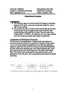
Figure 1.2.: Illustration of the events/landmarks related to the stop consonants considered in this thesis. The sub-phonetic events occurring during the production of a typical stop consonant are marked.

signal using an extended concept of the PI, called the dynamic plosion index. We demonstrate the efficacy of the proposed algorithm on several large corpora comprising simultaneous recordings of speech and electroglottographic signals under clean and noisy conditions. We compare our algorithm with the state-of-the-art algorithms and demonstrate its advantages over them. Epoch extraction serves as a necessary first step in all the algorithms proposed in the subsequent chapters on stop analysis and thus it is described first in the thesis. In Chapter 3, we address the problem of automatically locating the burst-onset landmarks of stops from continuous speech. This helps in ascertaining the interval around which the speech signal is to be analyzed to extract the phonetic features related to stops. We apply the same temporal measure PI defined in Chapter 2 on the pre-processed speech signal to locate the instants of abrupt change in energy. We use a pitch-synchronously derived cross-correlation based measure to reduce the false insertions. We devise a nonlinear classification algorithm to detect the burst onsets of stops using the aforementioned measures. We validate the proposed algorithm on several databases of read, continuous and telephone-quality speech using receiver operating characteristics curves. We also test the noise tolerance and scalability of the algorithm using noisy speech and databases of Dravidian languages, respectively. We also show that our algorithm compares well with the 14

1.6 Objectives and organization of the thesis state-of-the-art methods despite its simplicity. In first part of Chapter 4, we use the information of locations burst onsets to estimate the voice onset time of stops. We propose an algorithm devoid of requirement of a priori transcription and statistical training. We use pitch-synchronous innerproduct and zero-crossing patterns of stops and associated phones to devise an algorithm to estimate the voice-onset time. We validate our algorithm using multiple hand-labeled databases and demonstrate its effectiveness compared to the existing algorithms. We also show the utility of VOT in discriminating voiced from unvoiced stops and also in differentiating stops from affricates. In the second part of this chapter, we propose a method based on the dynamic plosion index to estimate the closure duration of the stops and validate the same. Chapter 5 deals with the classification of stops based on their place-of-articulation. We propose new features motivated from the differences in the temporal structures of the stops with different place of articulation. We show through experiments on large databases that temporal features can be as effective as spectral features whereas the combination of temporal and spectral features can increase the classification accuracy, confirming the presence of complementary information. The final Chapter concludes the thesis with a summary of the contributions and possible directions for future research. In the appendix, we explore the inter-domain applicability of the features and algorithms proposed in this thesis. Specifically, we apply the concept of dynamic plosion index to solve the problem of detection of QRS complexes from the electrocardiogram (ECG) signals. The proposed algorithm does not make use of any threshold. We show that it is computationally simpler than the existing algorithms through several experiments on the standard datasets.

15

2. Epoch Extraction using Plosion Index This chapter deals with the problem of detection of instants of significant excitation to the vocal tract called the epochs. Epoch extraction is a necessary first step in many speech analysis techniques, including those described in the later parts of this thesis. A temporal measure named the plosion index (PI) is proposed to locate transients in a time series. An algorithm is proposed to extract epochs from continuous speech using an extension of the PI called the dynamic plosion index. The proposed algorithm is validated using several databases comprising simultaneous recordings of speech and electroglottographic signal and it is shown to be comparable to the state-of-the-art techniques in terms of identification rate, accuracy and noise robustness.

2.1. Introduction The production of voiced speech is accompanied with a periodic source excitation signal arising due to the air-flow through the glottis which closes and opens periodically. The interval between successive glottal closures is termed as the pitch period. Flanagan defined epoch as the instant of significant excitation within a pitch period; He remarked, “presumably if such an epoch could be determined, the pulse excitation of a synthesizer could duplicate it and preserve natural irregularities in the pitch period” [37]. Miller proposed inverse filtering technique and used it to deduce that epoch lies close to the instants of periodic glottal closures which 17

Chapter 2

Epoch Extraction using Plosion Index

occur during the production of voiced sounds [22]. The significance of epochs in speech analysis has motivated a large number of researchers to address the problem of automatic identification of epochs or glottal closure instants (GCIs) from speech signals. In the rest of this chapter, we prefer to use the term epoch since it is signal-based in contrast to GCI which is a physiological term. In pitch-synchronous analysis of the voiced speech signal, epochs are used to define the analysis frames. That is, every analysis speech frame constitutes the samples within the interval between a pair of successive epochs. Epochs are also utilized in various speech processing applications including: (i) pitch tracking - the interval between successive epochs gives an estimate of the instantaneous pitch period, (ii) voice source estimation using closed-phase glottal analysis - here epochs are used to identify the interval over which the residual error is to be minimized to estimate the vocal-tract transfer function [38], (iii) speech synthesis [39] - in concatenation-based speech synthesis epochs are used to defined the units which are to be concatenated. This avoids perceptual glitches which arise if arbitrarily segmented units are concatenated. They are also used in prosody modification [40], (iv) speaker identification [41, 42] - Here epochs are used to accurately model the voice source whose characteristics are then used in a speaker recognition system, (v) speech enhancement - this is based on the observation that the segmental signal to noise ration (SNR) of the speech signal around epochs is higher compared to other locations [43], (vi) epochs have been shown to be useful in estimating the time delay between the speech collected from different microphones separated spatially [44]. Further, in this thesis, it will be shown that epoch-based processing can be used in voiced-unvoiced classification, manner class identification and VOT estimation. More information on significance of epoch based speech analysis may be found in [45, 46]. A primary requirement for such analysis based on epochs is the knowledge of the precise locations of the epochs or GCIs. Hence, the automatic detection of the epochs or GCIs from the voiced speech signal is considered to be an important problem in speech research and has been addressed by several 18

2.1 Introduction researchers [47, 48, 49, 50, 51, 52, 53, 54, 55, 56, 57, 58]. In the next section, a brief and critical review of five popular state-of-the-art methods viz., Hilbert Envelope (HE) based detection, the Dynamic Programming Phase Slope Algorithm (DYPSA), the Zero Frequency Resonator-based method (ZFR), the Speech Event Detection using the Residual Excitation And a Mean-based Signal (SEDREAMS) and the Yet Another GCI Algorithm (YAGA), proposed for epoch extraction is presented.

2.1.1. Epoch extraction - A review Broadly, there are two major steps in most of the epoch extraction algorithms: (a) Pre-processing of the speech signal to obtain a representation where epochs are significantly manifested, (b) selection of appropriate candidates corresponding to the epochs from the pre-processed signal. Since epoch is a characteristic of the excitation source signal, many works starting from [48, 47] consider the linear prediction residual (LPR) and its variants as a choice for pre-processing. It is hypothesized that epochs are manifested as local peaks in LPR and its varients such as Hilbert envelope (HE) of LPR. Motivated by such observations, some methods use center of gravity [49] and Gabor filtering [55] of the HE of the LPR for pre-processing. Subsequently, negative zero-crossings of the pre-processed signal are taken to be the epoch locations. However, a recent study [2] has shown that these approaches give the lowest scores in terms of five different performance measures considered. Smiths and Yegnanarayana [51] proposed the use of a signal arrived at by computing the mean group delay (GD) of a frame of the LPR samples centered at every sample, as an alternative to the HE of LPR. Here the candidates for epochs happen to be positive-going zero-crossings. However, this method is said to suffer from insertions [54]. Hence Naylor et al proposed DYPSA [54] algorithm where Dynamic Programming (DP) technique, with several suitably defined cost functions, was applied on the candidates derived from GD function to select the most appropriate candidates and reduce the number of insertions. 19

Chapter 2

Epoch Extraction using Plosion Index

The cost function is derived to exploit the characteristics of the voiced speech as such quasi-periodicity, waveform similarity, normalized energy etc. A similar method, YAGA [58] selects zero-crossing candidates of the GD function computed on the multiscale product of voice source signal instead of the LPR. Subsequently, DP technique is applied as in DYPSA to select the most appropriate candidate and reduce insertions. The accuracy of YAGA outperforms those of other techniques. Both these techniques, DYPSA and YAGA, are experimentally found to offer lower performance in the presence of noise. The poorer performance in the presence of noise may arise due to the pre-processing. Further, techniques using DP employ parameters optimized for clean speech, which might be inappropriate for noisy speech. To alleviate these problems, ZFR [56] and SEDREAMS [57] have been proposed which operate directly on the speech signal instead of LPR. ZFR is based on the fact that the effect of discontinuity in excitation is present over all frequencies. This comes from the assumption that the excitation signal for voiced speech can be approximated by a quasi-periodic impulse train which has equal components over all frequencies. Hence, in principle, analysis over any frequency band should possess epochal information. In ZFR based epoch extraction, a twostage double integrator (which acts as as a Zero Frequency Filter) has been used on the pre-emphasized speech signal for pre-processing. However, this introduces a dominant low frequency trend which is removed by a mean subtraction process repeated thrice. Positive-going zero-crossings are declared as the selected candidates. This method has tremendous noise robustness. However, ZFR method has a relatively lower accuracy (percentage of detected epochs within ±0.25 ms of the ground truth). SEDREAMS, a method motivated by ZFR, simplifies the preprocessing by using a mean based signal where the mean is computed by applying a Blackman-Tukey window over an appropriately selected interval. The GCI is assumed to lie within a fuzzy interval of the pre-processed signal around the zerocrossings and the exact location is postulated to be the major discontinuity in the LPR within that interval. This method retains the advantages of noise robustness 20

2.1 Introduction of ZFR and an improved accuracy which arises due to the use of the LPR for refinement. Although HE based methods also use the LPR, it is surprising that their reported accuracy [2] is lowest. A recent study has shown that the frequency response of ZFR resembles that of a lowpass filter [59]. The mean based signal computed in SEDREAMS using a symmetric Blackman-Tukey window is equivalent to convolving the speech signal with the FIR filter whose frequency response is that of a low pass filter. The pre-processing of ZFR and SEDREAMS can thus be interpreted as equivalent to lowpass filtering. We believe that it is the lowpass filtering which is providing the noise robustness in these methods. For speech signals with a relatively attenuated fundamental (or stronger second harmonic) as in the case of telephone quality or high pass filtered speech, these methods result in increased number of insertions. In ZFR and SEDREAMS, the global average pitch period has to be known a priori. This average pitch period determines the window length for trend removal in ZFR and running average computation in SEDREAMS. This parameter is shown to be critical [57] in the sense that an inappropriate value degrades the performance. For a given database, with both male and female speakers and also for a database where the mean pitch period may vary over a wide range, the average pitch period has to be estimated and specified for each speaker. Further, for emotional speech and singing voices where there are significant changes in the pitch period, estimated value of the average pitch period may be insignificant. If the average pitch period is known a priori then identification of epochs becomes simpler. An approach such as assuming the current epoch to be known and choosing the immediate next epoch as the maximum value in the speech signal within ±40 % of the assumed average pitch period, with random initialization can be adopted. When such an approach is experimented on a male speaker database (CMU Arctic BDL), it gave an identification rate of about 95 % at 0 dB SNR (with additive white noise) with an accuracy of about 57 %. On clean speech, it yielded about 97.5 % identification rate with about 70 % accuracy. 21

Chapter 2

Epoch Extraction using Plosion Index

2.1.2. Objectives of the current work From the above discussion on the existing techniques one can ascertain that rather than just identifying epochs, a bigger challenge lies in detecting epochs when the average pitch period is unknown and in achieving a higher accuracy. Motivated by aforementioned facts, in this chapter, we propose a non-linear signal processing algorithm for the identification of epochs with the following key features. 1. It operates on the half wave rectified integrated LP residual. 2. It selects the epochal candidates using a new non-linear temporal measure named the Plosion Index. 3. It does not assume the signal to be periodic and is independent of the energy contour. 4. It does not require a priori information of the average pitch period. 5. It does not depend on thresholds and cost functions. The proposed method is validated using the entire CMU ARCTIC [60] and APLAWD [61] databases, which provide simultaneous recordings of speech and electroglottograph (EGG) signals. Illustrations of the performance of the algorithm on some special cases are also provided. It has been tested in the presence of additive white as well as babble noise. The results are compared with five state-of-the-art algorithms in terms of all the performance measures recently reviewed in [2]. Further, it has also been tested on simulated telephone quality speech and the performance is compared with ZFR, SEDREAMS and DYPSA.

2.2. Proposed method The three major steps of the algorithm which are presented in this section are 1. Obtaining the half-wave rectified and negated ILPR as the pre-processed signal. 22

2.2 Proposed method 2. Dealing with the effect of the phase on ILPR. 3. Using plosion index to determine the immediate next epoch, assuming the current epoch is known.

2.2.1. Pre-processing A two level pre-processing technique is proposed which is explained in this section.

2.2.1.1. Integrated linear prediction residual Voiced speech is often modeled as the output of the vocal tract filter excited by a quasi periodic sequence of the derivative of glottal pulses. Epochal information is inherent in the derivative of glottal pulses, referred to as the voice source. Often, source signal and the vocal tract transfer function are estimated using the popular Linear Prediction (LP) techniques [62], [63] applied on the pre-emphasized speech signal. In LP analysis, the goal is to estimate every speech sample as a linear combination of a finite number of past speech samples. Mathematically, if s[n] represents the speech signal,

s[n] =

p X

ak s[n − k] + e[n]

(2.1)

k=1

where p is the number of previous samples used for estimation (referred to as the prediction order), e[n] is the error in the estimation, also called the LP residual. In the Z-domain, equation 2.1 can be written as

S(z) = S(z)

p X k=1

E(z)

ak z −k + E(z) =⇒ S(z) = 1−

p P

(2.2)

ak z −k

k=1

Since the vocal tract configuration changes continuously with time, the vocal tract filter is time-varying. However, to facilitate the analysis, the speech signal is assumed to be quasi stationary, i.e, stationary for a short interval of time, of the 23

Chapter 2

Epoch Extraction using Plosion Index

order of a few milliseconds, within the analysis interval. Now from the source-filter model of the speech production, speech signal s[n] is represented as the output of the convolution product of the glottal flow derivative signal ug [n] 1 and the impulse response of the vocal-tract filter h[n]. Mathematically,

s[n] = ug [n] ∗ h[n]

(2.3)

S(z) = Ug (z)H(z)

(2.4)

Equivalently in Z-domain,

1

If the vocal-tract filter is modeled as an all-pole filter, i.e, if H(z) = 1−

p P

,

ak z −k

k=1

then from equation 2.4 and equation 2.2 we have Ug (z) = E(z) =⇒ ug (n) = e(n). In LP-based inverse-filtering, the usual practice is to estimate the coefficients ak (called the LP coefficients) by minimizing the l2 − norm of the ‘error signal’. Mathematically,

ak ∗ = argmax k e(n) k2

(2.5)

ak

. This optimization problem is solved using one of the two approaches viz., the autocorrelation method or the covariance method, whose details can be found in [64]. The intuition behind minimizing the norm of the source signal is the assumption that the source-signal resembles an impulse-train which is sparse. However, it is known that the excitation source is not impulsive but has a quasi-periodic pulselike (as shown in Fig. 2.1) structure with a harmonic spectrum. Hence, in practice, 1

Strictly speaking, the excitation signal is the volume velocity waveform ( as shown in top trace of Fig. 2.1) but not its derivative. However, in practice, the effect of the lip-radiation, modeled as a differentiator, is combined with the volume velocity waveform and it is assumed that the derivative of the volume velocity drives the vocal-tract filter.

24

2.2 Proposed method

Glottal flow

1.5

Return Phase

Opening Phase

1

Closed Phase

0.5

Glottal−flow derivative

0

10

20

30

40

50

60

70

80

90

100

110

120

10

20

30

40

50 60 70 Sample number

80

90

GCI 100 110

120

1 0 −1 −2

Figure 2.1.: Illustration of one cycle of a typical glottal flow wave and its derivative. the speech signal is pre-emphasized prior to inverse filtering. Pre-emphasis is a filter with a transform function P (z) = 1 − αz −1 where α is close to unity. This filter compensates for the spectral tilt introduced by the source-signal and flattens the spectrum, validating the impulse-train assumption of the source signal. Pre-emphasis also facilitates the reduction of spectral dynamic range and thereby emphasizing the high-frequency regions. The pre-emphasized speech signal filtered with the inverse of vocal-tract filter (inverse filtered) yields the LP residual (LPR) which looks like an impulse train. Instead, if the inverse filtering is done directly on the speech signal, the resulting signal is referred to as integrated LP residual (ILPR) which closely approximates the voice source signal [65]. Fig. 2.2 illustrates the procedure in estimating the LPR and ILPR from speech signal. It is noteworthy that, pre-emphasis is a necessary first step in estimation of the LP coefficients. In case pre-emphasis is not applied before computing the LP coefficients, the inverse filtered signal tends to be noisy due to the improper cancellation of the high frequency components. Fig. 2.3 illustrates the effect of pre-emphasis on estimation of ILPR. Figure Fig. 2.3 (a) is the ILPR and Fig. 2.3 (b) is the signal obtained without using pre-emphasis in both the stages, on a segment of voiced speech. It can be noted that if pre-emphasis is not used while estimating the LPCs, the inverse filtered signal looks noisy whereas the use of pre-emphasis ensures that the estimated signal closely resembles the voice-source signal. 25

Chapter 2

Epoch Extraction using Plosion Index

Figure 2.2.: Illustration of the LP-based inverse filtering technique to obtain the LPR and ILPR. Strictly speaking, the term voice source signal refers to the inverse filter output when the filter is tuned accurately to the formant data estimated over the closed-glottis interval. In the present work, ILPR is obtained by inverse filtering the speech signal, with LP coefficients calculated on the pre-emphasized Hanning windowed speech samples using the autocorrelation method by setting the number of predictor coefficients to the sampling frequency in kHz plus four. For the current problem, the analysis is carried out using short-time windows of duration 18 milli-seconds (as described in the latter sections) and thus the LP-coefficients are computed once for each window. Since the inverse filter is not tuned accurately to the formant data, we prefer to use the term ILPR instead of voice source in this work. The locations of maximum negative peaks in ILPR are the representatives of the epochs. The epochal information is reflected as local peaks both in LPR and ILPR. However, in LPR, it has been noted that there are multiple bipolar peaks around the epoch [48], which makes unambiguous epoch extraction difficult [56]. This is because, pre-emphasis, a differencing operation, enhances high-frequency components. However, in ILPR, since there is no pre-emphasis, the peaks corresponding to epochs are less ambiguous. A 5-point symmetric moving averaging applied on 26

2.2 Proposed method −3

10

x 10

5 (a)

0 −5 50

100

150

200

250

300

350

400

−3

x 10 10 5

(b)

0 50

100

150

200 250 Sample number

300

350

400

Figure 2.3.: Illustration of effect of pre-emphasis on estimation of ILPR. Figure (a) is the ILPR and (b) is the signal obtained without using pre-emphasis in both the stages, on a segment of voiced speech. It can be noted that if preemphasis is not used while estimating the LPCs, the inverse filtered signal looks noisy whereas the use of pre-emphasis ensures that the estimated signal closely resembles the voice-source signal. ILPR further reduces the ambiguity. Henceforth, we refer to this smoothed version of ILPR simply as ILPR. As an illustration, Fig. 2.4 compares ILPR, Fig. 2.4(d and e), for a voiced speech segment shown in Fig. 2.4 (a) with LPR, Fig. 2.4 (b) and HE of LPR, Fig. 2.4 (c). There are local peaks around the epochs in LPR along with undesired components. Although HE of LPR is relatively a better representation, methods based on HE [49, 55] are shown to have poorer performance. It may be observed that the negative peaks in ILPR near epochs are relatively unambiguous compared to peaks in LPR and peaks in HE of LPR.

2.2.1.2. Half wave rectification It is known that volume-velocity air flow or glottal pulse reaches a peak and then decreases during the closing phase and thus has a negative slope. It has three phases the open phase during which the glottis is open allowing the air to freely flow through it. This is followed by a short return phase during which the vocal folds are snapping shut and there is a closed phase during which the glottis is shut (Fig. 2.1). At or near closure, the pulse has a maximum discontinuity with 27

Chapter 2

Epoch Extraction using Plosion Index

1 0 −1

(a) 100

0.2 0 −0.2

200

300

400

500

600

700

(b) 100

200

300

400

500

600

700

0.25 0.2 0.15 0.1 0.05

800

(c) 100

200

300

400

500

600

700

0.2 0 −0.2

800

(d) 100

200

300

400

500

600

700

0.1 0 −0.1 −0.2 −0.3

800

(e) 100

200

300

400 Sample number

500

600

700

800

Figure 2.4.: Illustration of manifestation of the epochs in various pre-processed signals. (a) A voiced speech segment, (b) LPR, (c) Hilbert envelope of LPR, (d) ILPR, (e) smoothed ILPR.

a negative slope [8]. Thus in general, the excitation to the vocal tract primarily manifests as a large negative peak in the glottal flow derivative. Since ILPR is an approximate estimate of the glottal flow derivative, the positive going part in the ILPR contains no information about the instant of the glottal closure as observed in the bottom trace of Fig. 2.1. Since the goal of this study is to estimate the glottal closure instant, ILPR is half-wave rectified by retaining only the negative part. Further, the rectified signal is negated. Here, we have assumed that the speech signal to be processed is of appropriate polarity; that is the ILPR resembles the natural voice source, wherein the closure interval is relatively shorter than the opening interval resulting in a larger negative peak than the positive peak. However, if the entire speech signal is reversed in polarity due to recording conditions, then the speech signal has to be negated before epoch extraction. It has been shown that methods like ZFR and SEDREAMS too have to address this issue [66] ; That is, the type of zero-crossing (positive/negative) associated with the epochs are reversed if the polarity of the speech signal is reversed. Hence, one may use automatic methods for polarity detection such as the one proposed in [66]. In the corpora considered in this 28

2.2 Proposed method study, there is no case of polarity reversal and hence we stick to clipping-off the positive-going part of ILPR in this work. Fig. 2.5 illustrates LPR, ILPR, and negated half-wave rectified ILPR (HWILPR) for a segment of voiced speech with additive babble noise at 0 dB segmental SNR. This segment is taken from Noizeus database [67] wherein the noisy signal is generated by adding noise to the speech signal filtered with a simulated telephone channel filter. The active speech level of the filtered signal is first calculated and then the noise samples are scaled and added to achieve the desired segmental SNR. This is to make the SNR independent of the silence segments which may be present in a given utterance. Such a noisy speech segment is shown in Fig. 2.5 (a). It is clearly seen that the HWILPR has the least ambiguity in spite of the presence of noise. 0.1 (a)

0 −0.1 5

10

15

20

25

30

35

40

45

0.02 0 −0.02

(b) 5

10

15

20

25

30

35

40

45

0.02 0 −0.02 −0.04 0.05

50

50 (c)

5

10

15

20

25

30

35

40

45

50 (d)

0

5

10

15

20

25 Time in ms

30

35

40

45

50

Figure 2.5.: Illustration of the reduction of ambiguity associated with ’peaks’ in ILPR corresponding to epochs through half wave rectification. (a) Voiced speech segment with additive babble noise at 0 dB segmental SNR, (b) LPR, (c) ILPR, (d) ILPR after half-wave rectification and negation (HWILPR).

2.2.1.3. Effect of the phase on ILPR Inverse filtering of voiced speech using LP technique does not always compensate the phase response of the vocal tract filter exactly. It has been observed that the effect of phase angles of different formants influence the wave-shape of LPR in a 29

Chapter 2

Epoch Extraction using Plosion Index

complex way [48]. Hence the phase of the vocal tract filter affects the shape of the estimated ILPR as well. ILPR resembles the natural voice source signal for some speakers whereas for others the phase (π/2 radians) shifted version of ILPR, i.e, the Hilbert transform of ILPR (HTILPR) agrees well with the natural voice source signal. Fig. 2.6 illustrates both ILPR and HTILPR for speakers belonging to these two categories. In Fig. 2.6 (a), ILPR resembles the natural voice source signal but, HTILPR appears almost as a rectangular wave; this signal reaches the base-line after a prolonged closing phase and possesses an abrupt bipolar swing preceding (or following) the negative peak. These characteristics deviate from the expected natural voice source pulse shape based on the physiological considerations. Similar observations may be noted with respect to ILPR for the speaker corresponding to Fig. 2.6 (b), whereas HTILPR agrees well with the expected shape of the natural voice source. From this, it appears that either the ILPR or the HTILPR has to be used as pre-processed signal depending on the speaker. Although the choice of ILPR or HTILPR does not affect the identification rate of epochs, it is useful for an accurate location of epochs 2 . This speaker-specific variation in the shape of the ILPR needs a deeper investigation and is beyond the scope of the present study since the interest of this study is to accurately extract the epochs. Henceforth we refer to half-wave rectified version of the appropriate signal (ILPR or HTILPR) as HWILPR for simplicity of notation.

Further, it is seen that when the ILPR is the appropriate choice, the maximum amplitude at the negative peak in ILPR is greater than that in HTILPR and vice-versa when the choice is HTILPR for a given cycle. Based on this, the choice of appropriate signal to be used for detecting the epochs for a given utterance is determined automatically using an algorithm described below.

2

Phase shift causes the negative peak in ILPR to get shifted only by a few samples, typically of the order of 1 ms and hence does not affect the identification rate.

30

2.2 Proposed method ILPR

−3

5

x 10

HTILPR

0

(a)

−5 2

4

6

8

10

12

14

16

18

20

22

−3

4 2 0 −2 −4

x 10

(b)

2

4

6

8

10 12 Time in ms

14

16

18

20

22

Figure 2.6.: Illustration of the effect of phase-shift on ILPR for two different speakers. (a) ILPR and HTILPR for a speaker. (b) ILPR and HTILPR for another speaker. For the case shown in (a), ILPR resembles the natural voice source signal and for that shown in (b), HTILPR resembles the natural voice source signal.

2.2.1.4. Algorithm for ascertaining the choice of appropriate signal for analysis

1. A given utterance is divided into non-overlapping frames of 40 ms for LP analysis.

2. Only those frames which have at least 10% of the highest energy, voiced frame within the utterance are considered. This ensures that frames which constitute low-energy unvoiced regions are discarded.

3. ILPR and its Hilbert transform (HTILPR) are estimated for each frame.

4. The ratio of the absolute value of the maximum negative peak in ILPR to that in HTILPR is calculated for each cycle.

5. The median of such ratios is calculated.

6. If the median is greater than one then ILPR is taken to be the appropriate signal else HTILPR is used. 31

Chapter 2

Epoch Extraction using Plosion Index

2.3. Temporal features 2.3.1. Plosion Index The goal now is to identify the instants corresponding to epochs, in the preprocessed signal, HWILPR. For this, we adopt a time domain measure which detects the transients in a signal. Transients may be defined as impulse-like events occurring in a signal. Stop bursts are typical examples of such transients occurring in speech signal. It is important to detect such discontinuities in continuous speech for performing burst detection, voice onset detection, landmark detection etc. We propose a sample measure named plosion index (PI) for detecting such transients. Intuitively, for a signal with a transient (characterized by a significant change in local energy), the ratio of the peak amplitude in the transient to the average of absolute values over an interval of interest excluding the instant of the peak, may be expected to be very high. In order to capture the intrinsic nature of a transient-like signal, we define the temporal measure PI at an instant of interest n0 for any signal s[n] as

P I(n0 , m1 , m2 ) =

|s(n0 )| savg (n0 , m1 , m2 )

i=n0X −m1 −1

where

savg (n0 , m1 , m2 ) =

(2.6)

|s(i)|

i=n0 −(m1 +m2 )

m2

(2.7)

when m1 and m2 are the number of samples corresponding to appropriately chosen intervals preceding n0 and

i=n0 +m X1 +m2

savg (n0 , m1 , m2 ) = 32

i=n0 +m1 +1

m2

|s(i)| (2.8)

2.3 Temporal features when m1 and m2 are the number of samples corresponding to appropriately chosen intervals following n0 . The values to be chosen for m1 and m2 depend on the specific application. PI is a dimensionless measure since it is a ratio and is independent of the recording level. The definition of PI is general in the sense that the values of m1 and m2 need not be on one side of the point of interest. One can define m1 and m2 symmetrically or asymmetrically around the point of interest, depending upon the specific application. To illustrate the usefulness of PI for the purpose of detecting the transients (stop bursts), we consider a segment of speech signal consisting of a fricative followed by a stop followed by a vowel. Fig. 2.7 illustrates the PI computed (using Eq. 2.8 for savg ) at every sample, n0 with m1 and m2 corresponding to intervals of 6 and 16 ms respectively. PI is relatively high (above 500) around the stop burst (160 ms) and low elsewhere. Hence, an appropriately chosen threshold on PI can detect a transient. The concept of PI has been applied and validated for the detection of bursts associated with stops and affricates which will be described in next chapter.

Amplitude

1 0.5 (a) 0 −0.5

20

40

60

80

100

120

140

160

180

200

220

Plosion index

600 400 (b) 200 0

20

40

60

80

100 120 Time in ms

140

160

180

200

220

Figure 2.7.: Illustration of the use of plosion index (PI) to capture transients. (a) A segment of speech signal with a fricative followed by a stop followed by a vowel, (b) plot of corresponding values of the PI. 33

Chapter 2

Epoch Extraction using Plosion Index

The definition of plosion index may remind a reader of the measure crest factor or peak-to-average ratio existing in the literature [68]. However, crest factor is defined as an index for an entire signal, where both the peak and the average values are derived from the complete signal. In contrast, PI is an instant measure. Also, PI is a function of two parameters (m1 ,m2 ) at any given instant. Further, since PI is designed to capture the ’departure’ of the amplitude at a given sample from the local trend, the computation of the average excludes the instant at which PI is being calculated. This makes PI to be a non-linear measure unlike crest-factor measure which is linear.

2.3.2. Dynamic plosion index In order to measure inter-epoch interval, we define an extended temporal feature named the dynamic plosion index (DPI). DPI is PI computed as a function of varying m2 for a given n0 and m1 using Eq. 2.9 for savg . Assuming that the lowest pitch to be extracted is 65 Hz which corresponds to a pitch period of approximately 15 ms, m2 is varied over a range corresponding to an interval of 0 to 15 ms. DPI is a vector of dimension 1 × N where N is the extent of variation of m2 . In the present context, m2 is to the right of current epoch n0 which is assumed to be known and the variable m1 is chosen to be -2. The problem is to identify the immediate next epoch. We shall see later how to initialize the process for the current epoch.

3

DPI computed for HWILPR (Fig. 2.8 (a)) of a voiced segment is depicted in Fig. 2.8 (b) (solid blue line). There are four pitch peaks in HWILPR. As m2 increases past the reference instant, marked as n0 in Fig. 2.8 (a), DPI gradually increases, reaches a peak and then decreases when m2 begins to include the signal corresponding to next cycle. It attains a local minimum around the peak in HWILPR which is close to the next epoch. Similar behavior is repeated for the subsequent cycles as 3

In principle, PI itself can be applied for determining the next epoch. However, in such a case, there would be a need to determine a threshold which should be applied on PI. To avoid such a requirement, we have defined DPI to capture the next epoch.

34

2.4 Epoch Extraction illustrated by the dotted red line in Fig. 2.8 (b), corresponding to DPI computed 0

at the dominant peak in the next cycle marked as n0 . .

HWILPR

0.03 0.02 (a) 0.01 0 0

n0

n0’ 100

50

150

200

250

DPI at n0 and n0’

Time in number of samples

600

DPI at n0 DPI at n0’

400

(b) 200 0

50

100

150

200

250

Value of m2 in number of samples (offset by n0 and n0’)

Figure 2.8.: Illustration of determination of next epoch given the current epoch using DPI. (a) HWILPR of a voiced segment, (b) DPI ( with m1 = −2) com0 puted with reference to n0 and n0 on the signal in Fig. 2.8 (a) are shown in solid blue line and dotted red line, respectively.

2.4. Epoch Extraction 2.4.0.1. Initialization As mentioned earlier, the problem is posed as that of determining the next epoch given the current epoch. This requires a knowledge of the current epoch. It has been found that the proposed method is insensitive to the initialization for the very first cycle which may be done arbitrarily. Subsequently, the estimated epoch location is used for initialization for the next cycle.

2.4.0.2. Determination of successive epochs Having known the current epoch, the next epoch is detected as follows. 1. DPI of HWILPR is computed with the current epoch as n0 . 35

Chapter 2

Epoch Extraction using Plosion Index

2. The peaks and valleys in the DPI are computed by detecting the positive and negative zero-crossings in its derivative, respectively.

3. As noted previously, each peak-valley pair in HWILPR corresponds to a cycle. The absolute difference in the values of DPI at each peak-valley pair is computed.

4. It is evident from Fig. 2.8 (a) and Fig. 2.8 (b), that the peak-valley pair with the largest difference corresponds to the immediate next cycle. The time instant corresponding to such a valley is noted.

5. Thus, the instant of peak in HWILPR within ±2 ms of the valley determined in the previous step, is hypothesized as the estimate of the immediate next epoch.

6. The above procedure is repeated over the entire speech signal irrespective of voiced/unvoiced regions.

The proposed algorithm is henceforth referred to as DPI algorithm. Fig. 2.9 illustrates the flowchart for the entire algorithm. Fig. 2.10 shows a segment of voiced speech along with the corresponding DEGG signal (whose negative peaks are considered the ground truth) and the epoch locations estimated using the DPI algorithm. It may be seen that the epochs are correctly determined irrespective of the signal energy and also their locations nearly coincide with the negative peaks in DEGG signal. 36

2.4 Epoch Extraction

Figure 2.9.: Flowchart for the DPI algorithm for epoch extraction.

1 0.5 (a) 0 −0.5 400

450

500

550

600

650

700

750

800

850

0.05 (b)

0 −0.05 −0.1 400

450

500

550

600

650 Time in ms

700

750

800

850

Figure 2.10.: Illustration of the epochs estimated by the proposed algorithm. (a) A segment of voiced speech, (b) Estimated epoch locations (top trace), DEGG signal (bottom trace). 37

Chapter 2

Epoch Extraction using Plosion Index

2.5. Evaluation 2.5.1. Databases considered and the performance measures 2.5.1.1. Comparison with DEGG signal It has been shown that negative peaks in DEGG signal are very close to the instants of glottal closure [69, 70]. Epoch extraction techniques are often validated by considering negative peaks in DEGG signal as the ground truth. The DPI algorithm is validated only on the voiced segments of any given utterance since epochs are meaningful only for voiced segments. Voiced-Unvoiced decision is made by applying a negative threshold on DEGG signal. A previous study [71] has used 1/6 times the peak-to-peak value of DEGG as the threshold for V-UV decision. However, we use a worse case choice of (1/9) times the maximum negative value of the DEGG signal for a given utterance so that even low energy voiced segments are captured. The compensation for the delay between the EGG signal and the acoustic signal captured by the microphone is done manually for each speaker and is assumed to be constant for all the utterances of the speaker in the database.

2.5.1.2. Databases Six large databases containing speech and simultaneous EGG recordings are used for validation. The first five are from CMU ARCTIC databases. The first three contain 1132 phonetically balanced sentences. Each of these are single speaker databases corresponding to BDL-US male, JMK-Canadian male and SLT-US female. The fourth database contains non-sense words containing all phone-tophone transitions in English uttered by a male speaker (RAB-UK male). The fifth database contains 452 sentences used in TIMIT databases uttered by a male speaker (KED-US male). These are available in public domain in Festvox webpage [60]. APLAWD [61] is the sixth database consisting of five English sentences repeated five times by five male and five female speakers. It has been mentioned 38

2.5 Evaluation in [2], that the all pass equalization filter used in this database for correcting low frequency phase distortion has no effect on GCI detection. This database has been obtained from the author of [57]. Table 2.1 lists the number of true epoch candidates (obtained from the DEGG signal) in each of these databases. Table 2.1.: Summary of databases used for validation. Name of the Database

BDL (1-Male) SLT (1-Female) JMK (1-Male) KED (1-Male) RAB (1-Male) APLAWD (5-Males, 5-Females) Total number of true epochs

No. of epochs (duration in min) 218802 (54) 338875 (55) 152510 (54) 64072 (20) 67176 (29) 114430 (20) 955865 (232)

2.5.1.3. Performance measures We employ the same performance measures as those described in many of the recent studies [2, 56, 54] which are illustrated in Fig. 2.11. A glottal cycle is defined as the interval from (ei − ei−1 )/2 to (ei + ei+1 )/2 , where ei is the ith reference epoch derived from DEGG signal. The following are the definitions of the performance measures used. 1. Identification rate (IDR) : Ratio of number of glottal cycles with only one epoch detected per cycle to the total number of glottal cycles. 2. Miss rate (MR) : Ratio of number of glottal cycles with no epoch detected within that cycle to the total number of glottal cycles. 3. False alarm rate (FAR) : Ratio of number of glottal cycles with more than one epoch detected per cycle to the total number of glottal cycles. 4. Standard deviation of error (SDE) : The standard deviation of distribution of δ over an entire database where δ is the timing error between the true 39

Chapter 2

Epoch Extraction using Plosion Index

and the detected epoch locations in ms. This is sometimes referred to as the identification accuracy (IDA) in the literature [2]. 5. Accuracy to ±0.25 ms : The proportion of detected epoch candidates with δ less than 0.25 ms relative to the total number of identified epochs is yet another performance measure which is of interest. The first three of the above are collectively called the reliability measure and the

Detected epochs

Reference epochs

others are called the accuracy measures. 1

0.5

0 0

0.1

0.2

0.3

0.4

0.5

0.6

0.7

1

0.9

1

0.9

1

δ False insertion

0.5 Miss 0 0

0.8

0.1

0.2

0.3

0.4

0.5 Time

0.6

Identification

0.7

0.8

Figure 2.11.: Illustration of the performance measures used in the current study.

2.5.2. Results on Clean Speech The results of the DPI algorithm validated on clean speech using the above performance measures, are given in Table 2.2. Also given are the results of algorithms with maximum and minimum performances amongst those compared (HE based, DYPSA, YAGA, ZFR, SEDREAMS) in a recent review paper [2]. In Table 2.2, algorithms SEDREAMS, DYPSA and YAGA have been abbreviated as SED, DYP and YAG, respectively. The fifth performance measure is considerably low for HE based method on all databases. Hence, while comparing that measure, we present the maximum and minimum amongst the remaining four algorithms along with the results of DPI algorithm. 40

2.5 Evaluation Table 2.2.: Summary of performance of the proposed algorithm on clean speech on six databases and comparison with other methods. Database

BDL

SLT

JMK

KED

RAB

APLAWD

IDR %

MR %

FAR %

SDE in ms

DPI - 99.11 YAG- 98.43 HE - 97.04 DPI - 99.47 ZFR - 99.26 HE - 96.16 DPI - 99.45 SED - 99.29 HE - 93.01 DPI - 99.64 SED - 98.65 ZFR - 87.36 DPI - 98.96 SED - 98.87 DYP - 82.33 ZFR - 98.89 DPI - 97.17 HE - 91.74

DPI - 0.15 YAG - 0.39 DYP - 2.12 SED - 0.12 DPI - 0.22 HE - 2.38 DPI - 0.16 SED - 0.25 HE - 3.94 DPI - 0.08 YAG - 0.63 ZFR - 7.90 DPI - 0.01 SED - 0.63 ZFR - 6.31 YAG - 0.52 DPI - 1.99 HE - 5.64

DPI - 0.75 ZFR - 0.98 DYP - 2.34 DPI - 0.31 ZFR - 0.59 DYP - 1.41 DPI - 0.39 ZFR - 0.40 HE - 3.05 DPI - 0.02 SED - 0.68 ZFR - 4.74 DPI - 1.03 SED - 0.50 DYP - 15.80 SED - 0.51 DPI - 0.84 HE - 2.62

DPI - 0.21 YAG - 0.29 HE - 0.58 DPI - 0.19 ZFR - 0.22 HE - 0.56 DPI - 0.24 YAG - 0.40 HE - 0.90 DPI - 0.17 SED - 0.33 HE - 0.56 DPI - 0.27 SED - 0.37 HE - 0.78 DPI - 0.34 SED - 0.45 HE - 0.73

Accuracy to±0.25ms % DPI - 92.17 YAG - 90.31 ZFR - 80.93 DPI - 89.29 YAG - 86.16 SED - 81.35 DPI - 88.53 SED - 81.05 ZFR - 41.62 DPI - 98.59 YAG - 95.14 ZFR - 46.82 DPI - 94.01 SED - 91.26 ZFR - 55.87 DPI - 89.13 YAG - 85.51 ZFR - 57.87

The reliability measure, IDR, of DPI algorithm is the highest for all CMU ARCTIC databases. For the APLAWD database, it it is slightly less than the best, but well above the lowest reported. Irrespective of the database, DPI algorithm’s IDR is more than 97%. As far as the standard deviation of timing error (SDE) and accuracy to ±0.25 ms are concerned, it is observed that DPI algorithm outperforms all other algorithms for all databases. For the speakers JMK, KED and RAB, the choice for the pre-processed signal happens to be HTILPR and for others the choice is ILPR. In case we use ILPR for JMK, the accuracy to 0.25 ms would fall down significantly to about 75% from 88%. Table 2.3 summarizes the IDR and accuracy performance measures for all the algorithms averaged over all the databases. For DPI algorithm, IDR averaged over all six databases is 99.13% which is the highest amongst all the algorithms compared.

Fig. 2.12 is a normalized histogram of the timing error of the DPI

algorithm averaged over all the six databases. Identified epochs which lie within 41

Chapter 2

Epoch Extraction using Plosion Index

±0.25 ms of the ground truth is 90.77% which is the highest. SDE is 0.23 ms for DPI algorithm which is the least amongst all the algorithms. These results may be due to the fact that DPI algorithm uses an appropriate choice of ILPR or HTILPR for pre-processed signal and rectification. The performance measures of YAGA algorithm is close to that of DPI algorithm, which may be explained by the fact that YAGA also uses the estimated voice source signal. The methods which use LPR or voice source for refinement give a better accuracy. This shows that epochs can be more precisely detected in these representations. In summary, the performance of the DPI algorithm is comparable to the best amongst the state-of-the-art algorithms, without the need for average pitch information and dynamic programming. 0.35 SDE = 0.236 ms 0.3

Accuracy to 0.25 ms = 90.77%

Probability

0.25 0.2 0.15 0.1 0.05 0 −1

−0.8

−0.6

−0.4

−0.2 0 0.2 Epoch timing error in ms

0.4

0.6

0.8

1

Figure 2.12.: Normalized histogram of epoch timing error made by the DPI algorithm over all databases.

2.5.3. Demonstration of the efficacy on some special cases In this section, we illustrate the efficacy of the DPI algorithm on typical examples of some special cases.

2.5.3.1. Voice-bar and nasal murmur To demonstrate the fact that the DPI algorithm is independent of the energy contour, we consider a segment of speech taken from the utterance “will Robin 42

2.5 Evaluation wear a yellow lilly” from KED database. This segment shown in Fig. 2.13 consists of a strong vowel followed by a weak-voice bar of a voiced-stop consonant followed by a vowel and a nasal. It also depicts the detected epochs and the DEGG signal. It is clear from Fig. 2.13 that the DPI algorithm detects epochs irrespective of the energy contour and even during the low-level voiced segments.

/aa/

/w/

Nasal /n/

/ax/

Voice bar of /b/

0.5 (a) 0 −0.5 600

620

640

660

680

700

720

740

760

780

800

0

−0.05

(b)

−0.1 600

620

640

660

680

700 Time in ms

720

740

760

780

800

Figure 2.13.: Demonstration of the independence of the DPI algorithm on the energy contour of the signal. (a) A segment of voiced speech comprising a strong vowel followed by a voiced stop consonant followed by a vowel and a nasal, (b) epochs determined from DPI algorithm (top trace), corresponding DEGG signal (bottom trace). DEGG has been shifted for illustrative purpose.

2.5.3.2. Creaky voice segment Since the DPI algorithm does not make quasi-periodicity assumption, it has been applied on an arbitrarily chosen segment of creaky voiced speech taken from Voqual03 database [72] (BrianCreak3.wav). Two important distinctions of creaky voiced speech from normal speech are (i) irregular periodicities with long pitch periods (ii) presence of secondary and tertiary excitations which may arise due to ventricular incursion [73]. Fig. 2.14 shows a segment of speech of creaky voice, along with the corresponding DEGG signal and the determined epochs. Locations of primary excitations are shown by solid lines and those of secondary excitations are shown by dashed lines. It may be seen from DEGG that there are irregular periodicities throughout the entire segment. DPI algorithm detects the primary 43

Chapter 2

Epoch Extraction using Plosion Index −3

x 10 5

(a)

0 −5 320

340

360

380

400

420

440

460

480

500

520

0

(b)

−0.5

−1 320

340

360

380

400

420 440 Time in ms

460

480

500

520

Figure 2.14.: Demonstration of DPI algorithm on creaky voiced segment. (a) A creaky voiced segment, (b) epochs determined by DPI algorithm (top trace), DEGG signal (bottom trace). DEGG has been shifted for illustrative purpose. Locations of primary excitations are shown by red solid lines and those of secondary excitations are shown by blue dashed lines. epochs for this difficult case. Although there is a missed detection around 360 ms, secondary excitations around 390, 410, 430 and 460 ms have been detected. A large scale study on the performance of epoch extraction on different voice qualities (breathy, creaky, loud etc.) as reported in [74] is a problem by itself which is beyond the scope of this study.

2.5.3.3. Singing voice Since the DPI algorithm does not require a priori pitch information, it is expected to perform reasonably well on singing voice where the pitch spans a very large range. To ascertain this, we validate the DPI algorithm on singing voice utterances taken from Voqual03 database [72], which consists of simultaneous EGG recordings. It consists of three singers - one male and two female. The number of true epochs is 3338. We also compare the results with ZFR and SEDREAMS which require a-priori average pitch information for epoch detection4 . Table 2.4 compares the reliability performance measures for the three algorithms on singing voice. It may be seen that the large variation of pitch does not degrade the perfor4

Average picth period was estimated from the DEGG signals and provided for ZFR and SEDREAMS.

44

2.6 Robustness aspects mance of the DPI algorithm whereas the performance of ZFR and SEDREAMS are relatively more affected.

2.6. Robustness aspects Some applications demand epoch extraction algorithms to be robust against various types of degradation in speech signal. In this section, we study the performance of the algorithms under two types of speech degradation namely addition of noise (white and babble) and bandwidth reduction as in telephone quality speech.

2.6.1. Noisy conditions 100

IDR (%)

1

10

1

80 10

70

70

0.9

1

60

0.8 0.7

60

50

0.6

0

50

10

0.5

40

0

40 0

80

1.1

90

Accu. to 0.25 ms (%)

SDE (ms)

FAR (%)

MR (%)

10 10

20

0

10

20

0.4 0

10

20

0

10

20

30 0

10

20

SNR in dB DPI

DYPSA

YAGA

SEDREAMS

HE based

ZFR

Figure 2.15.: Performance of six different algorithms over all databases at different SNRs (0 to 25 dB) with additive white noise. The values of performance measures for algorithms other than DPI method have been taken from [2]. Two types of noise are considered in the present study, a stationary white noise and a non-stationary babble noise or cocktail party noise. White noise generated from sampling a zero mean normal distribution is added to every utterance. The variance is set in accordance with the desired global SNR. Samples corresponding to babble noise are taken from Noisex-92 database [75], scaled and added to speech signal to achieve desired global SNRs. Fig. 2.15 and Fig. 2.16 depict the 45

Chapter 2

Epoch Extraction using Plosion Index FAR (%)

MR (%)

IDR (%) 2

2

10

100

10

90 90 1

1

10

80

SDE (ms) 1.6

10

Accu. to 0.25 ms (%) 90

1.4

80

1.2

70 70

1

60

0.8

50

0.6

40

0.4

30

70 0

0

10

10

60 50 40 0

−1

−1

10

20

10

0

10

20

10

0

10

20

0.2 0

10

20

20 0

10

20

SNR in dB

DPI

DYPSA

YAGA

SEDREAMS

HE based

ZFR

Figure 2.16.: Performance of six different algorithms over all databases at different SNRs (0 to 25 dB) with additive babble noise. The values of performance measures for algorithms other than DPI method have been taken from [2]. performance of six algorithms averaged over all databases under various SNRs for the two noise cases, respectively. Performance measures of the algorithms other than DPI are taken from the recent review paper [2]. In the case of white noise, it may be seen that the IDR of the DPI algorithm is almost unchanged and comparable to ZFR and SEDREAMS and is 96% at 0 dB SNR. The superiority of the accuracy performance of the DPI algorithm is retained even at 0 dB SNR. It has the lowest SDE at all SNRs and better accuracy below 15 dB SNR. Even at 0 dB SNR, almost 72% of the determined epochs are within 0.25 ms of the ground truth. In the case of babble noise, IDR of the DPI algorithm degrades gradually below 10 dB SNR from about 97% and reaches 87% at 0 dB SNR. This lowering of performance below 10 dB may be due to the model dependence. However, it is better than other model based techniques such as DYPSA, YAGA and HE. SDE of the DPI algorithm is lowest above 10 dB SNR, and becomes slightly higher than ZFR and SEDREAMS, below 10 dB. Accuracy to 0.25 ms of DPI algorithm remains highest at all SNRs. In summary, DPI algorithm is highly robust against white noise in terms of every 46

2.6 Robustness aspects performance measure considered and offers the highest accuracy at all SNRs. For babble noise, the performance is comparable to the best in the literature till 10 dB SNR below which it slightly degrades. However, the accuracy performance is superior for all SNRs. Table 2.3.: Performance measures averaged over all databases for various algorithms. Method DPI YAGA SEDREAMS ZFR DYPSA HE BASED

IDR in % 99.13 98.38 98.81 96.37 95.11 94.60

SDE in ms 0.23 0.34 0.34 0.42 0.44 0.67

Accuracy to 0.25 ms (%) 90.77 83.40 80.80 57.90 71.90 39.70

Table 2.4.: Performance of three algorithms on singing voice. Algorithm DPI ZFR SEDREAMS

IDR (%) 94.1 88.2 83.3

MR (%) 5.04 0.01 3.03

FA (%) 0.5 11.8 13.63

2.6.2. Telephone quality speech To examine the robustness of epoch extraction algorithms against bandwidth degradation as in telephone quality speech, we validate the performance of four algorithms viz., DPI, DYPSA, ZFR and SEDREAMS

5

on simulated telephone

quality speech, using the same performance measures as defined in the earlier section. Since a large database consisting of actual telephone channel speech with simultaneous EGG recordings is not available, we use simulated data. Telephone channel can be approximated by a bandpass filter (BPF) between 300 and 3400 Hz. We designed a BPF and used it to simulate the telephone quality speech. The magnitude response of the filter is defined in the frequency domain 5

DYPSA is implemented using the software Voicebox [76]. ZFR and SEDREAMS are implemented using corresponding authors’ codes.

47

Chapter 2

Epoch Extraction using Plosion Index

using a raised cosine function between 0 and 300 Hz, unity between 300 and 3400 Hz and again a raised cosine function from the folding frequency up to 3400 Hz. The speech signal is down-sampled to 8 kHz and the frequency domain implementation of BPF gives simulated telephone quality speech which is then used as input for the epoch extraction algorithms. The magnitude response of the simulated filter is shown in Fig. 2.17. 0 −5

Magnitude in dB

−10 −15 −20 −25 −30 −35 500

1000

1500

2000 2500 Frequency in Hz

3000

3500

4000

Figure 2.17.: Magnitude response of the filter used for simulating telephone quality speech.

The algorithms are evaluated on three databases namely BDL, KED and SLT, which cover male speakers of two different accents and one female speaker, respectively. The results are presented in Table 2.5. Table 2.5.: Results of various algorithms on simulated telephone quality speech. Database

BDL (male F0 ≈ 130 Hz)

KED (male F0 ≈ 105 Hz)

SLT (Female F0 ≈ 200 Hz) 48

Method

IDR (%)

MR (%)

FAR (%)

SDE (ms)

DPI ZFR SED DYP DPI ZFR SED DYP DPI ZFR SED DYP

97.69 42.05 83.72 95.07 93.44 30.19 78.70 98.12 98.66 99.28 99.18 96.15

0.04 0.01 0.02 0.05 0.04 0.07 0.01 0.04 1.01 0 0 0.09

1.87 57.95 16.26 4.37 6.14 69.75 21.29 0.14 0.03 0.07 0.08 2.92

0.20 0.28 0.31 0.35 0.26 0.97 0.36 0.28 0.28 0.19 0.33 0.41

Accuracy to 0.25 ms (%) 93.09 35.21 72.80 85.82 93.88 6.12 79.55 86.24 87.60 78.94 78.56 72.56

2.6 Robustness aspects The performance of ZFR and SEDREAMS degrade severely for male speakers since the resulting zero-frequency resonator output and mean-based signal, are not sinusoidal. As every zero-crossing is deemed as an epoch candidate, false alarms significantly increase. The degradation in the performance of SEDREAMS is less than that of ZFR. This is due to the fact that effective lowpass filter of ZFR is steeper than that used in SEDREAMS (frequency response of Blackman-Tukey window). Further, the performance is much worse in the case of the speaker KED. This is because, the relative spectral level of fundamental is lower for this speaker than that of the others even in clean conditions. This explains the lowest score of ZFR method for this speaker (87% IDR) under clean conditions whereas it is consistently more than 98% for all others. However, DPI method and DYPSA suffer very little degradation in the performance on telephone quality speech. This may be due to the absence of lowpass filtering. DPI method is not only reliable but also accurate. The scenario is completely different for the female speaker SLT. There is no degradation in the performance in any of the algorithms since the telephone channel does not degrade the fundamental. There is a slight lowering of accuracy in the case of SEDREAMS and ZFR.

2.6.3. Analysis of sensitivity to choice of pre-processed signal As mentioned in the earlier sections, some of the epoch extraction algorithms, such as SEDREAMS, ZFR and DPI are sensitive to the choice of polarity of the speech. In addition, DPI algorithm needs to ascertain the correct pre-processed signal (ILPR or HTILPR) for ensuring better accuracies. Albeit automatic algorithms are presented in the previous sections for knowing these choices, for the sake of completeness, in this section, we analyze the sensitivity of the DPI algorithm for these choices. In particular, we carry out two experiments where (i) utterances from BDL database are inverted in polarity and given as inputs to 49

Chapter 2

Epoch Extraction using Plosion Index

the DPI algorithm, (ii) incorrect choice of pre-processed signal (opposite to that said by the choice-detection algorithm) is fed as input. Table 2.6 summarizes the outcomes of the aforementioned experiments. Table 2.6.: Illustration of the sensitivity of the DPI algorithm on the choice of pre-processed signal. Measures Incorrect polarity Incorrect signal choice

IDR 98.1 99.1

MR 3.5 0.2

FAR 1.4 0.7

SDE 0.48 0.25

Accu. 0.25 ms 4.9 89.1

In the case of polarity reversal, it is seen that there is not much degradation in the IDR value (98.1 % from 99.1 %). However, the accuracy to 0.25 ms reduces drastically from 90 % to 5 %. This is understandable since the clipping of negative part of ILPR makes the GCI information to vanish albeit the glottal opening instants will be detected making the IDR intact. For the second experiment, there is only a slight reduction (3%) in the accuracy to 0.25 ms measure as claimed in previous sections.

2.7. Conclusion In this chapter, we have proposed an algorithm, named the DPI algorithm, for epoch extraction. Half wave rectified and negated integrated linear prediction residual is used as the pre-processed signal which appears to be relatively less ambiguous to identify epochs than other signal representations. The effect of phase of formants on ILPR has been dealt with appropriately. A new temporal measure, Plosion Index proposed to detect ’transients’ in speech signals has been used. An extension of PI, called the Dynamic Plosion Index (DPI) is applied on the preprocessed signal to detect the epochal candidates. The method has been validated against EGG recordings using six large databases comprising 15 speakers. It is tested for its robustness in the presence of additive white and babble noise. Also, robustness is studied on simulated telephone quality speech. The performance of DPI algorithm is compared with several state-of-the-art algorithms. It has been 50

2.7 Conclusion found that the performance of DPI algorithm is comparable to the best in the literature, for all the cases studied. DPI algorithm is effective even for low-level voiced segments. It does not require a priori pitch information which suggests that it may be applied to speech with large range of pitch as in the case of emotional speech or music.

51

3. Burst-onset landmark detection for stops and affricates In this chapter, the problem of automatic detection of instants of closure-burst transitions or the burst-onsets of stops and affricates is dealt with. Burst-onset is a primary landmark associated with the stop consonants around which most of the analysis are carried out for stops. A knowledge-based algorithm is proposed using the temporal measures plosion index and maximum normalized cross-correlation. The proposed algorithm is validated using several databases of read, conversational and telephone speech and its performance is found to be comparable to the state-of-the-art techniques despite its simplicity.

3.1. Background During the production of stops [77], acoustic pressure is built up behind a closure at a place within the vocal tract, resulting in a silent interval or a low level acoustic signal, with or without voicing. When the pressure is released suddenly, it introduces a relatively high energy burst or transient in the acoustic signal, spanning a short interval. The production of an affricate consonant (/ch/ and /jh/ in English) is also similar to that of a stop consonant [77]. They share the properties of both the stops and fricatives. The instant in the acoustic signal corresponding to the sudden release is referred to as the ‘burst-onset’ [15] or the closure-burst boundary or the closure-burst transition (henceforth abbreviated as the CBT). The problem 53

Chapter 3

Burst-onset landmark detection for stops and affricates

of automatic detection of the CBTs of stops and affricates from a continuous speech signal is recognized as important in several studies [15, 3, 4, 78, 79]. Although we consider detecting CBTs of both stops and affricates here, in the next chapter, we demonstrate a method for discriminating stops from affricates. In the remaining part of this section, we briefly discuss the problem as relevant to (i) automatic speech recognition (ASR) and (ii) acoustic-phonetics studies. Subsequently, we review the methods proposed in the literature for detection of the CBTs. As described in the introduction chapter, approaches to ASR may be classified broadly into two classes. The ones based on statistical models primarily employ hidden Markov models (HMMs) and a generic acoustic feature such as Melfrequency-cepstral-coefficients (MFCCs) common to all the phones [80, 7]. Alternative approaches are based on initially deriving the phonetic-feature-specific information from the speech signal, followed by the identification of phones [23, 18, 17, 81]. A landmark-based ASR system is an example of the latter approach where ‘events’ in the speech signal with rapid temporal and spectral changes, called the landmarks, are extracted in the initial stage. The subsequent step is to analyze the speech signal only around the landmarks to derive acoustic information for the purpose of classification of phones [18]. Automatic detection of the CBTs is of relevance to both the types of ASRs; it has been shown that the performance of an HMM-based ASR system can be enhanced by incorporating the information of the CBTs along with the MFCCs [4]. The detection of the CBTs plays a role in identifying the burst-onset landmark, a manner class called ‘stops’ or the distinctive feature called ‘interrupted’ in other ASR systems [23, 82, 83, 15]. In acoustic-phonetics studies, detection of the CBTs has been shown to help in the identification of the appropriate analysis interval for determining the place of articulation of stops [84]. Further, voice onset time (VOT) is noted to be a significant attribute useful for the discrimination of voiced from unvoiced stops [85]. VOT also aids in accent identification, clinical applications, etc [86]. State-ofthe-art methods proposed for automatic measurement of VOT require an a-priori 54

3.1 Background knowledge of the CBTs [87]. Thus, automatic detection of the CBTs caters to this need. Further, CBTs are needed to estimate the closure intervals of stops which are shown to aid manner and place classification of stops [88].

3.1.1. Burst-detection - A survey In the literature, the methods proposed to detect burst-onset landmarks, stopbursts, manner class ‘stop’ and stop consonants rely on the temporal and/or spectral characteristics of the speech signal around the CBTs for feature extraction and on the labeled CBTs as the ground truth for validation [3, 4, 79, 82, 89, 15, 78]. We briefly review all these methods by noting the acoustic feature and the classification strategy used. For detecting the stop-bursts, Bitar [89] used the degree of abruptness in energy difference between two appropriately located frames as an acoustic measure, which was originally proposed by Espy-Wilson [90], in a ‘fuzzy’ rule-based classifier. Liu [15] used the rate-of-rise of energy (RoR) across appropriately located frames in six specific frequency bands and a threshold-based logic to detect stop-burst landmarks. King and Taylor [82] have used short-time energy and MFCCs along with their derivatives (39 parameters) as the feature vector and trained neural networks to identify all the sound-pattern-English (SPE) features proposed by Chomsky and Halle [21]. Hou et al. [83] utilized a range of temporal and spectral acoustic features (energy ratios, zero-crossings, linear prediction coefficients etc.) as inputs to classifiers such as multi-layer perceptron and Bayesian classifier to extract all the SPE features. These features were subsequently used to detect stop consonants. Lin and Wang [4] have used a two-dimensional cepstrum as the feature vector (56 dimensional) and a random forest (RF) classifier for detecting burst-onset landmarks. Niyogi et al. [78] used three energy measures (log of total energy, log of energy above 3 kHz and Wiener entropy) as a feature vector in a support vector machine (SVM) classifier to detect stop consonants. Niyogi and Sondhi [3] used the same feature vector with an optimal adaptive filter consisting of 33 parameters to detect stop consonants. Salomon et al. [19] have used 55

Chapter 3

Burst-onset landmark detection for stops and affricates

four temporal features to detect acoustic landmarks and used them in a HMM classifier to identify several manner classes including ‘stop’. Jayan and Pandey [79] used a Gaussian mixture model (GMM) of smoothed log magnitude spectrum (256 coefficients) and the rate of change of the components of the (GMM) to detect stop consonants. Generally, these methods are validated against a labeled database, with marked closure-burst boundaries, such as the TIMIT database. A common criterion is that if the detection is within a certain temporal tolerance (20-40 ms) of the labeled closure-burst boundary of a stop/affricate, then the method is deemed to have detected the burst-onset landmark or a stop/affricate consonant or the manner class ‘stop’. The performance is characterized in terms of false acceptance and rejection rates (and the associated receiver operating characteristic-ROC curve) by some methods and in terms of deletion and insertion rates by others. Also, the statistics of the temporal deviation of the detected CBTs from the labeled boundary are considered for characterizing the accuracy of detection.

3.1.2. Objectives of this work In this work, we propose two new temporal features and a rule-based classifier for the detection of the CBTs and find out if it can result in a performance comparable to the best reported in the literature for similar experimental conditions. Also, we study the robustness and scalability of the proposed method. Formally, the objectives of this work are: (a) To propose and use a one-dimensional temporal measure to detect events with abrupt increase in energy such as the CBTs of stops. (b) To design a rule-based algorithm (without the need for statistical training), to select a subset of these events belonging to stops and affricates using a second temporal feature. (c) To validate the algorithm on the entire TIMIT training and test databases with criteria similar to those used in the previous studies [4, 3] and to characterize the performance by the ROC curves. (d) To test the robustness 56

3.2 Temporal measures of the algorithm in the presence of two types of additive noise, viz., stationary white noise (global and local SNRs) and non-stationary babble noise and also on telephone quality speech (using the NTIMIT database). (e) To test the scalability of the algorithm on the Buckeye corpus comprising conversational speech and a database of two Indian languages.

3.2. Temporal measures Research into finding new temporal measures and their application in speech processing is recognized as an important area [19]. It has been suggested that temporal measures are relatively robust and that human perception also makes use of temporal cues [91]. In this section, we describe the use of the temporal measure named the plosion index (PI) proposed in Chapter 2 to detect events with abrupt change in energy. Sometimes such a change in energy (as seen around the CBTs) is also observed in events like strong voiced onsets preceded by a low-level signal. In sec. 3.2.3, one more temporal measure, namely the maximum normalized cross-correlation (MNCC), is proposed to discriminate a CBT from a voiced onset.

3.2.1. Manifestation of stop bursts in continuous speech The acoustic signature of an ideal or a typical stop production is a sudden release of energy preceded by a closure. During the production of stops and affricates, bursts are supposed to manifest as abrupt transients in the speech signal. However, in continuous speech, stop bursts manifest in a variety of styles making the problem of burst detection challenging. Since the proposed method is based on temporal analysis, we illustrate in Fig. 3.1 examples of stops manifesting widely varying temporal characteristics. Most of the unvoiced and voiced stops possess impulselike structures with a strong burst preceded by a well-defined closure without and 57

Chapter 3

Burst-onset landmark detection for stops and affricates

with voicing (Fig. 3.1 a) during the closure interval. There may be multiple bursts even for a single stop, especially for /k/ (Fig. 3.1 b). For some of the voiced stops, the burst manifests as a small amplitude high frequency ‘kink’ in one of the voiced cycles, mostly occurring during the last cycle (Fig. 3.1 c). Some bursts corresponding to unvoiced stops may show a gradual build-up and decay instead of a sudden change in amplitude (Fig. 3.1 d). Occasionally, a burst may be weak or even unreleased.

Figure 3.1.: Different manifestations of stop bursts. (a) An impulse-like voiced stop burst, (b) multiple bursts of /k/, (c) a weak burst with a high-frequency ’kink’ over-riding on the pre-voicing in a voiced stop, (d) an unvoiced stop burst with a gradual build up and decay of amplitude.

3.2.2. The Plosion index (PI) In order to capture the intrinsic nature of a transient-like signal preceded by a low-level signal, as in a CBT of a stop, we reinforce the concept of PI defined in Chapter 2. The PI at an instant of interest n0 for a signal s[n] is defined as follows

P I(n0 , m1 , m2 ) = 58

|s(n0 )| savg (m1 , m2 )

(3.1)

3.2 Temporal measures

i=n0 −(m1 +1)

X

where savg (m1 , m2 ) =

|s(i)|

i=n0 −(m1 +m2 )

m2

(3.2)

is the average of the absolute amplitudes of m2 samples, offset from n0 , by m1 samples . In the context of the detection of the CBTs of stops/affricates from a continuous speech signal, an appropriate choice needs to be made for m1 and m2 . Since certain low-level noise-like signal components, called the pre-frication, are usually present preceding the instant of maximum amplitude within an unvoiced stop-burst [3], we choose m1 as the number of samples corresponding to 6 ms (see Sec.V.A for a justification for this choice). This excludes the samples of pre-frication (which are of amplitude higher than those in the stop-closure region) while computing savg . Based on the statistics of the minimum closure duration for stops [92], m2 is chosen as the number of samples corresponding to 16 ms. Throughout this work, m1 and m2 are kept fixed corresponding to these chosen values. Fig. 3.2 illustrates the role of m1 in enhancing the value of the PI, through an example of a stop (/k/), shown in Fig. 3.2 (a), occurring at a consonant cluster (/s/-/k/). Fig. 3.2 (b) and (c) show the corresponding PI values computed (at the peaks between every successive zero-crossings) without and with the use of the offset m1 while computing the savg , respectively. The presence of a strong pre-frication may be observed resulting in lower values of the PI in Fig. 3.2 (b). However, the PI values almost increase two-fold (Fig. 3.2 (c)) when the offset m1 is used.

3.2.2.1. Pre-processing for the computation of the PI The change in energy around the CBT is low for a voiced stop with a weak release preceded by a relatively strong pre-voicing component. Fig. 3.3 (a) shows 59

Chapter 3

Burst-onset landmark detection for stops and affricates −3

x 10 2 1 0 −1

/s/

/k/

/kcl/

/m/ (a)

200

400

600

800

PI

10 (b)

5 0

200

400

600

800

PI

10 (c)

5 0

200

400 600 Sample index

800

Figure 3.2.: Illustration of the need for offset m1 in reducing the effect of prefrication on the PI. (a) A segment of speech with a fricative followed by a stop, (b) the corresponding PI values computed without the offset m1 , (c) the corresponding PI values with the offset m1 .

an example of such a case. At the instant of release n0 , the PI computed on this signal is about 4. In order to attenuate the pre-voicing component preceding such a CBT and thereby enhance the amplitude contrast, the speech signal is high-pass filtered with a cut-off frequency of 400 Hz [15]. However, this does not significantly influence the abrupt change in the amplitude around the CBTs of unvoiced stops and affricates (as may be seen in Fig. 3.2). Fig. 3.3 (b) shows the high-pass filtered signal corresponding to the same segment shown in Fig. 3.3 (a). Now, at the instant of release n0 , despite a decrease in the peak value, the PI increases to about 16. The intervals corresponding to m1 and m2 are also marked in Fig. 3.3 (b). It has been noted that the excitation strength of an impulse-like signal is better 60

3.2 Temporal measures 0.08 0.06 0.04 0.02 0 −0.02 −0.04

PI = 4

100

200

300

400

500

0.08 0.06

600

PI = 16

0.04 0.02 0

m1

m2

−0.02 −0.04 100

200

300 Sample index

400

n0 500

600

Figure 3.3.: Illustration of the utility of the high-pass filtering for reliable detection of the CBTs of voiced stops. (a) A segment of a voiced stop with a weak release, (b) the corresponding segment after high-pass filtering. It may be seen that there is an increase in the value of the PI by a factor of 4, after high-pass filtering. represented by the peak in its Hilbert envelope (HE) [93]. This is due to the following observation: In the case of an ideal impulse, the strength of excitation is represented by the peak amplitude. However, if there is a shift in the phase of the impulse, for example as in the case of Hilbert transform of an impulse, the strength of excitation is represented by the peak to peak amplitude of the signal or the peak amplitude of its HE as illustrated in Fig. 3.4. Since stop-bursts are impulse-like signals, the PI is computed on the Hilbert Envelope (HE) of the high-pass filtered speech signal, for the current application. Hilbert transform is computed in the time domain by convolving the speech signal with a 32-point finite impulse response of the Hilbert transformer. Fig. 3.5 illustrates the PI values computed at every sample for a segment of a speech signal consisting of a fricative followed by a stop followed by a vowel. The PI is high (>600) around the CBT (126 ms) and low elsewhere. It may be observed from Fig. 3.5 that there is an interval (marked by dashed vertical lines) around the CBT within which the PI is high. However, since the CBT is an instant, it is desirable to have only one candidate representing a transient interval. To reduce the interval measure to an instantaneous measure, we propose a merger rule, which 61

Chapter 3

Burst-onset landmark detection for stops and affricates 1

Hilbert transform (HT) of an impulse Hilbert envelope of the HT

Amplitude

0.5

0

−0.5

−1 0

5

10

15 20 Sample number

25

30

35

Figure 3.4.: Illustration of use of Hilbert envelope in enhancing the peak amplitude. It is seen that the peak amplitude of the HE is almost twice that of the signal. is explained as a part of the detection algorithm in sec. 3.3.

3.2.2.2. Discriminability of the PI In order to test the discriminability of the PI for detecting the CBTs against other events, the normalized histograms of representative PIs for (a) stops/affricates and (b) other phones (vowels, semi-vowels, glides, nasals and fricatives) from the entire labeled TIMIT database are computed and shown in Fig. 3.6. The maximum value of the PI within a labeled segment is taken to be the representative PI for that phone. A total of 19866 tokens of stops and affricates and 89552 tokens of other phones are considered. Although a large separation of the two classes is seen, there is a considerable overlap. For example, if one chooses a threshold of 8 for the PI to separate the classes, 93% of the CBTs of stops and affricates would be detected correctly. However, 33% of other phones would be incorrectly classified as the CBTs. This is because the PI detects abrupt onset corresponding to any sound preceded by a low-level signal. It is observed that most of these arise from the strong onsets of voiced sounds which are to be discriminated from the CBTs of stops and affricates. For this purpose, we define yet another temporal measure, called the maximum normalized cross-correlation. 62

3.2 Temporal measures 0.5

(a)

0

−0.5 20

40

60

80

100

120

140

160

0.6 0.4

(b)

0.2 0

20

40

60

80

100

120

140

160

600 400

(c)

200 0

20

40

60

80 100 Time in ms

120

140

160

Figure 3.5.: Illustration of the ability of the PI to capture events with abrupt increase in energy. (a) A segment of a speech signal with a fricative followed by an unvoiced stop followed by a vowel, (b) the Hilbert envelope of the high-pass filtered speech, (c) the PI corresponding to the signal shown in (b), computed with m1 and m2 corresponding to the time intervals of 6 and 16 ms, respectively.

3.2.3. The maximum normalized cross-correlation It is well known that normalized cross-correlation (NCC) quantifies the degree of similarity as a function of the lag between two finite energy signals, irrespective of their energies [94, 95]. In this work, the maximum value of the NCC (MNCC) is used as the second temporal feature. By definition, the MNCC is a scalar and lies between 0 and 1. In the literature, NCC is generally computed between the segments of a speech signal, of about 20-40 ms in duration, for the purpose of pitch estimation and voiced-unvoiced decision [94]. However, in the present work, we compute NCC between the segments of speech over two successive inter-epoch intervals. This assumes that the epochal information is available. Epochs are extracted using the DPI algorithm proposed in the previous chapter of this thesis. The value of the MNCC, computed between two successive inter-epoch intervals, is assigned to all the samples over the first inter-epoch interval. Thus, the MNCC plotted for a speech signal appears as a staircase-like function. 63

Chapter 3

Burst-onset landmark detection for stops and affricates 0.16

PI for stops and affricates PI for other phones

0.14

Probability

0.12 0.1 0.08 0.06 0.04 0.02 0 0 10

1

2

10

3

10

10

PI in logarithmic scale

Figure 3.6.: Normalized histograms of the PI for stops/affricates (solid line) and other phones (dashed line) of the entire TIMIT database. The x-axis is shown in logarithmic scale for clarity. The overlap between the two groups in higher values of the PI is largely due to strong voiced onsets. For a speech signal corresponding to a voiced sound, the vocal tract impulse responses for successive pitch periods are highly correlated, resulting in a high value for the MNCC. There is no such high-correlation between two successive segments in the case of unvoiced sounds due to the random excitation, which results in a lower MNCC. Fig. 3.7 shows a speech segment (a stop followed by a vowel, a fricative and another vowel) with the corresponding values of the PI and the MNCC. The MNCC is low (typically less than 0.6) for the unvoiced regions and high (typically greater than 0.6) for the voiced regions. 0.4 0.2 0 −0.2 −0.4

(a)

50

100

150

200

250

300

350

PI

720

(b)

0

10

50

100

150

200

250

300

350

MNCC

1 (c)

0.5 0

50

100

150 Time in ms 200

250

300

350

Figure 3.7.: Illustration of the use of the maximum normalized cross correlation (MNCC) to separate the CBTs from the voiced onsets. (a) A speech segment, (b) the corresponding PI values, (c) the corresponding MNCC values, showing MNCC values greater than 0.6 for the voiced segments.

In order to test the discriminability of the MNCC for voiced-unvoiced classification, 64

3.2 Temporal measures we compute the normalized histograms (Fig. 3.8) of the average MNCC within the labeled regions for the two classes of phones from the TIMIT database; class-A consists of a total of 29150 tokens of unvoiced stops, affricates and fricatives; classB consists of a total of 73016 tokens of vowels, semi-vowels, glides and nasals. The histograms show a clear separation of the two classes with a negligible overlap area of less than 5% for both the classes at a threshold of 0.6. Thus, in this work, MNCC for unvoiced phones MNCC for voiced phones

0.3

Probability

0.25 0.2 0.15 0.1 0.05 0 0

0.2

0.4

0.6 MNCC

0.8

1

1.2

Figure 3.8.: Normalized histograms of the MNCC values of voiced (dashed line) and unvoiced sounds (solid line) from the entire TIMIT database. The overlap area is about 5% in either case at a threshold of 0.6. a threshold of 0.6 is used on the average MNCC computed over three successive inter-epoch intervals to exclude strong voiced onsets being detected as the CBTs. For example, in Fig. 3.7, though the value of the PI is high at the vowel onsets, they may be identified as not belonging to the CBTs since the average MNCC around those onsets is above 0.6. Around the CBT of a voiced stop, the MNCC will have a high value due to the presence of quasi-periodicity. Hence, there is a risk of these CBTs being discarded as voiced onsets. However, a singular feature of the voiced stops is a disruption of the periodicity over one or two cycles coinciding with the release, which results in a significant ‘high-low-high’ structure in the MNCC around the CBT. Fig. 3.9 (a) shows one such instance. Thus, the ‘high-low-high’ structure in the MNCC can be used to detect the CBTs of such voiced stops. Further, the MNCC may be high even in the case of multiple bursts of a single unvoiced stop, thus may be discarded as a voiced onset. This is because the signals corresponding to the individual bursts may be correlated with one another. Fig. 3.9 (b) shows an example of an unvoiced 65

Chapter 3

Burst-onset landmark detection for stops and affricates

stop with multiple bursts, along with the plot of the corresponding MNCC. This case of multiple bursts is dealt with using the ‘number of potential candidates’, defined in the next section. 1 0.5

(a)

0 −0.5 65

70

75

80

85

90

95

0.6 0.4

(b)

0.2 0 −0.2 1295

1300

1305

1310

1315

1320

Time in ms

Figure 3.9.: (a) Illustration of the ‘high-low-high’ structure of the MNCC for a voiced stop with a weak burst; (b) An unvoiced stop with multiple bursts resulting in MNCC > 0.6.

3.3. The CBT detection algorithm We formulate certain rules to select the CBTs based on the knowledge derived by studying a number of typical cases. In other words, we ‘learn the rules through examples’. The following are the steps in the algorithm illustrated by the flowchart in Fig. 3.10. 1. The PI is computed only at the locations of the maxima of HE between every set of successive zero-crossings of the high-pass filtered signal. 2. The instants at which the PI is greater than a threshold (T 1 ) are called the potential candidates. 3. Based on the assumption that no two genuine stop (affricate) releases occur within 20 ms of each other [4], any two successive potential candidates that are within 20 ms of each other are postulated to belong to one and the same event. In this algorithm, only the very first potential candidate within such 66

3.3 The CBT detection algorithm

Speech signal

Epoch extraction

Highpass filtering

Feature extraction

Zero-crossings (ZCs) MNCC between inter-epoch intervals

Hilbert envelope (HE)

PI of HE at max. between ZCs

RBC and Nc

............................................................................................................................................................................................................................................

No

PI > T1?

Potential candidates

Yes

Yes

No

MNCC around RBC has a high-low-high structure ?

Yes Instant is not a CBT

RBC is not a CBT

No

MNCC post RBC > T2?

Nc > T3?

No

Decision rules

Yes

RBC is a CBT

RBC is a CBT

RBC is a CBT

Weak voiced burst

Multiple bursts

Strong burst

Figure 3.10.: Flowchart of the proposed APR algorithm for detection of the CBTs. an event is retained and is called representative burst candidate (RBC). The number of potential candidates (Nc ) within that event is noted. This step is to ensure that there is only one RBC per CBT. This is referred to as the merger rule. 4. When the average MNCC over three successive inter-epoch intervals immediately following the RBC exceeds a threshold T 2 , three possibilities arise. a) RBC is a CBT of unvoiced stop with multiple bursts: This is confirmed when Nc exceeds a threshold (T 3 ). This is based on the observation that 67

Chapter 3

Burst-onset landmark detection for stops and affricates the number of potential candidates is significantly higher for multiple bursts than for onsets of voiced sounds.

b) RBC is a CBT of a voiced stop: This is ascertained by a local high-lowhigh structure in the MNCC around RBC. c) RBC is not a CBT (e.g., strong voiced onset): If neither of the above cases is satisfied, then RBC is removed from further consideration. 5. When the average MNCC over three successive inter-epoch intervals immediately following RBC is less than the threshold T 2 , RBC is declared to be a CBT of a stop/affricate. The choice for the values of the thresholds is discussed later. The output of the proposed algorithm, called the detector output, is a vector with unit impulse at the detected CBTs and zero elsewhere. The proposed algorithm, hereafter called the APR algorithm, not only detects the CBTs, but also the type of burst such as voiced with a weak release, multiple bursts, unvoiced or voiced bursts with a relatively strong release. This is ascertained by the path traversed in the algorithm to arrive at the detector output. The maximum value of the PI within an event may be used as a measure of the strength of release. We illustrate in Fig. 3.11, a segment of a speech signal (of the utterance ‘put the butcher block table in the garage’) along with the detector output obtained using the optimal thresholds. There are correct detections of the CBTs for the stops /p/, /b/, /b/, /t/, /b/, /g/ and the affricate /ch/. There is a detection for the dental fricative /dh/ around 900 ms since dental fricatives occasionally tend to be ‘stop-like’ [96]. However, around 2200 ms, there is a case of /dh/ without a release, and hence there is no detection. In the region labeled as a closure, /kcl/, around 1600 ms, there is a detection which may be interpreted as incorrect [4]. However, we interpret this detection as belonging to a genuine CBT of an unlabeled /k/ in the consonant cluster (/k/ - /t/) occurring at a word boundary. It is recognized that the release may or may not be present for the former stop consonant in a 68

3.4 Evaluation procedure and experimental details cluster [97]. The labeling could have been /kcl/-/k/-/tcl/-/t/. Incidentally, there is a consonant cluster /t/-/dh/ around 900 ms. However, the burst of /t/ is unreleased in this case and there is no detection 1 .

0.04

Amplitude

0.02 0 −0.02 −0.04 600

/p/

/tcl/ /dh/

800

/b/

1000

/ch/

1200

/b/

1400

/b/

/kcl/ /t/

1600

1800

2000

/dh/

2200

/g/

2400

2600

Time in ms

Figure 3.11.: Illustration of the detected CBTs for a segment of a speech signal of the utterance ’put the butcher block table in the garage’ taken from the TIMIT test set. The detected instants are shown by vertical lines along with the corresponding TIMIT transcriptions at those locations.

3.4. Evaluation procedure and experimental details Since the goal of the APR algorithm is to detect the CBTs of the stops and affricates, these phones are said to belong to the target class. However, phones such as glottal-stops [98], flaps [99] and dental fricatives [96] also may manifest the CBTs. Since the manifestation of the CBT is not consistent for these phones, detector outputs, if any, occurring during these labeled segments are excluded while calculating the performance measures. Previous studies [4] have also followed a similar criterion for these phones. All other phones are included in the rejection class. 1

Another example of a consonant cluster with two distinct releases occurs in the word ‘expectation’ in test-dr1-faks0-si943 of the TIMIT test database, between 2.85 and 2.99 s. A burst corresponding to /k/ can be seen in that utterance around 2.918 s as confirmed by temporal and spectral characteristics.

69

Chapter 3

Burst-onset landmark detection for stops and affricates

3.4.1. Performance measures A labeled database is an absolute necessity for the validation of the CBT detection algorithm. We have adopted the standard performance measures described in the literature [3, 4] that are defined below. 1. Correct detection: A detection is considered to be correct if it lies within ±20 ms of the labeled closure-burst boundary. The tolerance of 20 ms is to account for any possible inaccurate boundary markings present in the databases [3]. 2. Missed detection: This occurs when there is no detection within ±20 ms of the labeled CBT of a phone from the target class. 3. False detection: A detection is considered false, if it occurs within the labeled region of a phone from the rejection class. 4. False acceptance rate (FAR): The number of false detections divided by the total number of phones from the rejection class. 5. False rejection rate (FRR): The number of missed detections divided by the total number of phones from the target class. 6. Temporal deviation of detection: The statistics of the deviations of the locations of the detected CBTs from the labeled boundaries, computed only for the correct detections [4].

3.4.2. Choice of thresholds and the ROC curves As one varies the thresholds for detection, there is a trade-off between FAR and FRR. Based on the risk factors and the application, one may like to make different choices for FAR and FRR and accordingly select the thresholds. Hence a knowledge of the nature of the trade-off between FAR and FRR is required. This is provided by the Receiver Operating Characteristic (ROC) for any detection problem, where FAR is plotted against FRR. When there is no specific preference 70

3.4 Evaluation procedure and experimental details for either FAR or FRR, then the performance is specified by the equal error rate (EER), which corresponds to that point in the ROC curve, where FAR=FRR. Hence we characterize the performance of the algorithm by means of the ROC curves and derive the EER from the same. The ROC may be obtained by varying the thresholds for the PI and the MNCC. Since the distributions of the MNCC values for voiced and unvoiced classes show a clear separation (an overlap area of less than 5% for either classes at a threshold of 0.6), we fix T2 at 0.6 and vary only the threshold T1 meant for the PI, to generate the ROC curves. T3 is fixed at 7, based on our empirical observations.

3.4.3. Databases and experimental setup We validate the proposed algorithm on three different labeled databases, which differ significantly in terms of speakers, dialects, recording conditions, speaking styles (read vs. conversational) and languages. These diverse conditions contribute to a wide variability in the acoustic characteristics of the speech signal. Also, we consider different types of degradations on one of the databases (TIMIT). This section describes all the experiments conducted.

3.4.3.1. The TIMIT database - clean speech

To validate the APR algorithm on read speech, we use the TIMIT [100] database which is labeled at the phone level. It consists of a total of 6300 utterances spoken by 630 speakers belonging to several dialects of North America. The database is divided into the training and test sets of eight dialects each, comprising 4620 and 1680 utterances, respectively. The APR algorithm has been validated on the entire TIMIT training and test databases independently. In TIMIT, the closure-burst boundaries are marked explicitly for all stops and affricates, which are taken as the ground truth for validation. 71

Chapter 3

Burst-onset landmark detection for stops and affricates

3.4.3.2. The TIMIT database with white and babble noise - global SNR

To study the noise robustness of the APR algorithm, we test it on the entire TIMIT test set with two types of additive noise, stationary white noise and realistic, non-stationary babble noise. White noise is generated using a zero mean Gaussian distribution whose variance is set in accordance with the desired global SNR. Samples of babble noise are taken from the Noisex-92 database [75] and appropriately scaled to obtain the desired global SNR. Though TIMIT utterances used in the test set have a mean SNR of 39.5 dB [3], in our calculations, we have assumed the speech to be clean. Thus the actual SNRs are slightly lower than the SNRs of 30, 20 and 10 dB reported in this study.

3.4.3.3. The TIMIT database with Schroeder noise - local SNR

The global SNR is predominantly determined by the strong voiced segments. Therefore, the local SNR around the CBTs would be much lower and not directly predictable. In order to study the performance of the APR algorithm at specific local SNRs around the CBTs, we have adopted the Schroeder noise model and the procedure given by Niyogi and Sondhi [3] for generating the noisy speech of a desired local SNR. According to this model, the noisy speech signal y(n) is generated at every sample n, using the formula y(n) = s(n)[1 + η(n)], where s(n) is the clean speech signal. η(n) is a binary valued (-1 and 1) random variable which takes on values -1 and 1 with equal probability at each n. Further it is ensured that η(n1 ) is independent of η(n2 ) for all n1 and n2 so that the noise thus generated has a flat power spectrum making it white.  is the design parameter which is determined by the specified local SNR. Three cases of local SNRs, namely 20,10 and 0 dB are used in this study. Only the TIMIT test set is considered in order to compare the results of the APR algorithm with the published results. 72

3.4 Evaluation procedure and experimental details 3.4.3.4. The NTIMIT database - telephone quality speech

To study the performance against channel degradation, we employ the NTIMIT test database [101], which is the telephone quality version of the TIMIT database. The utterances in NTIMIT differ from those in TIMIT in two important respects, namely, a reduction of bandwidth from 0-8000 Hz to 300-3400 Hz and a degradation in SNR from 39.5 to 26.8 dB [3].

3.4.3.5. The Buckeye corpus - conversational speech

To test the scalability of the algorithm on conversational speech, we consider the Buckeye corpus [102] consisting of several hours of recordings of spontaneous American English speech of 40 speakers from central Ohio, USA. Informal conversations were elicited by an interviewer in a seminar room with the speaker allowed to move freely. The corpus is phonetically labeled using a two stage labeling process involving forced alignment and manual correction. The corpus is available in the public domain [103]. In this corpus, the entire interval from the closure to the onset of the next sound (e.g., vowel onset), including the burst, has been assigned the label of the stop/affricate consonant. Hence, we modify the definition of the correct detection: a detection is defined to be correct if it lies anywhere within the entire region labeled as stop/affricate. Since there are no separate labels for closure and burst intervals, temporal deviations of detection cannot be measured. A randomly selected subset of the speech data from all the 40 speakers has been considered. Since the duration of each speech file is very long (of the order of ten minutes) and consists of several utterances with intermittent long pauses, any detection following a labeled long silence is ignored. The number of stops and affricates in the selected subset is 1972 and the number of phones from the rejection class is 11307. 73

Chapter 3

Burst-onset landmark detection for stops and affricates

3.4.3.6. The MILE database - Dravidian languages To further test the scalability of the algorithm, we consider the MILE database comprising about 2000 utterances of phonetically rich sentences of two Dravidian languages, Kannada and Tamil, spoken by male speakers (one for each language) annotated manually at the phone level. These were recorded in a studio environment for the purpose of the development of a text-to-speech synthesis system [104] in the MILE lab, Indian Institute of Science. Here, the CBTs are not explicitly labeled. Hence the performance evaluation is the same as that used for the Buckeye corpus. The target class includes all the stops and affricates of the corresponding languages. The number of tokens in the target and rejection classes is 2352 and 11700 for Kannada and 2359 and 13635 for Tamil databases, respectively.

3.5. Experimental results In this section, we present the results of the experiments in the same order as described in sec. 3.4.3. The results are compared with some state-of-the-art algorithms and summarized in Table 3.1. An analysis of errors is also presented with reference to the TIMIT database.

3.5.1. The TIMIT database - clean speech The ROC curves and EERs Fig. 3.12 depicts the ROC curves for the TIMIT training and test databases. It is noteworthy that there is very little difference in the ROC for the test and the training databases with equal error rates (EER-APR) of about 7.7% for the test and 7.9% for the training databases, respectively. Incidentally, EER is achieved around a threshold for the PI of 8 which corresponds to about 9 dB. In the literature, an energy difference of 9 dB has been used for the detection of stop 74

3.5 Experimental results bursts [105, 15]. In our study, it has been noted that if the PI alone is used for the CBT detection without the MNCC and the associated rules, EER increases to 12. 0.4 APR−TIMIT test APR−TIMIT train N&S EER−APR test EER−PI only EER−RF EER−N&S EER−SVM EER−GMM

0.35 0.3

FAR

0.25 0.2 0.15 0.1 0.05 0.02

FAR=FRR

0.04

0.06

0.08

0.1

0.12

0.14

0.16

0.18

0.2

FRR

Figure 3.12.: The ROC curves of the APR algorithm (solid line : TIMIT test database, dashed line : TIMIT training database) with the EERs compared with some state-of-the-art methods. FAR: false acceptance rate; FRR: false rejection rate. The ROC curve (dotted line - for a subset of the TIMIT test database) and EER for the N&S algorithm are taken from Niyogi and Sondhi’s paper [3]. EERs for RF, SVM and GMM are taken from Lin and Wang’s work [4].

In general, the CBTs of unvoiced stops are detected better than those of voiced stops. This may be because the burst release is weaker in the case of voiced stops. Specifically, the detection accuracy is the highest for /p/ (around 96%) and the lowest for /g/ (around 86%). For affricates, it is about 87%.

Temporal deviation To quantify the accuracy of the detected locations of the CBTs with reference to the labeled boundaries, we use the temporal deviation of detection. The deviation δi associated with each correct detection is defined as δi = ti − t∗i , where ti is the detected location and t∗i is the labeled closure-burst boundary in TIMIT. Fig. 3.13 shows the probability density function (normalized histogram) of δ and the cumulative distribution function of the absolute value of δ for the entire TIMIT test and training databases (combined together). The percentage of the detected CBTs are 64%, 84%, 97% and 100% for deviations of 5, 10, 15 and 20 ms, respectively. 75

Chapter 3

Burst-onset landmark detection for stops and affricates

probability

0.2 0.15

(a)

0.1 0.05 0 −30

−20

−10

0 δ in ms

10

20

30

probability

1 0.8 (b)

0.6 0.4 0.2 0

5

10

15

20

25

30

35

|δ| in ms

Figure 3.13.: Histograms of the temporal deviation δ for the TIMIT test and training databases combined. (a) PDF and (b) CDF. The mean deviation is 1.8 ms for unvoiced stops and 3.3 ms for the voiced stops. The standard deviation is 6 ms for unvoiced stops and 5.1 ms for voiced stops. The distribution of δ is skewed to the right because the hand-labeled boundary in TIMIT often precedes the actual location of the release as also noted by Lin and Wang[4]. A transcriptor may mark the closure-burst boundary at the beginning of the pre-frication interval. This may explain the skewness observed and justify the choice of m1 corresponding to an interval of 6 ms.

Comparison with the previous work

We compare the results of the APR algorithm with those of three state-of-the-art algorithms: RoR-based (denoted by ‘Liu’) [15], adaptive filtering approach (denoted by ‘N&S’) [3] and random-forest based (denoted by ‘L&W’) [4]. Strictly speaking, the results are not comparable because of the different sizes of the datasets considered and different criteria for the temporal tolerance for detection and differences in the target sets considered. The number of tokens considered for testing in our study is the highest amongst all the studies reported in the literature. Fig. 3.12 also shows the ROC curve of the N&S algorithm (manually read from their study [3] and re-plotted here) and the EERs achieved by the different algo76

3.5 Experimental results rithms. The trade-off between FAR and FRR is less severe in the case of the APR algorithm than the N&S algorithm. As an example, to achieve an FRR of 5%, the APR algorithm results in an FAR of 13% as against 32% of the N&S algorithm. The EER of the N&S algorithm is 16%, with affricates included in the rejection class. Lin and Wang report an EER of 7.3% using a RF classifier, 7.7% using an SVM classifier and 8.8% using a 16-component GMM on the TIMIT test set. These EERs are also indicated in Fig. 3.12. The EER of the APR algorithm for the TIMIT test set (7.7%) equals that of SVM and is marginally (0.4%) less than that of RF. However, in L&W’s study, a temporal tolerance of more than 30 ms is used for defining a correct detection. If the temporal tolerance is increased to 40 ms from 20 ms in the APR algorithm, the EER decreases to 7.2% from 7.7% on the TIMIT test set, which is better than that with both the RF and SVM classifiers used in L&W [4]. Lin and Wang have noted that the computational load of SVM makes it impossible to be used as an efficient burst detector. On the other hand, our proposed algorithm uses only two temporal measures and a simple rule based classifier. Liu has not reported the EER but reports 19% deletion (FRR) for stop-bursts with a temporal tolerance criterion for detection being 30 ms. Another study by Niyogi et al. reports an EER of about 13% using SVM classifier on a single dialect of the TIMIT test database [78]. The EER for this case is not shown in Fig. 3.12. In the L&W algorithm, the percentage of detections are 64%, 86%, 99.2% and 99.6% for temporal deviations of 5, 10, 20 and 30 ms, respectively. The corresponding results for the APR algorithm are 64%, 84%, 100% and 100% respectively. The mean and standard deviation of δ are 4.7 and 5.7 ms for the L&W algorithm compared to 2.7 and 5.8 ms for the APR algorithm on the test database. Given the aforementioned facts, the performance of the proposed algorithm appears significant, with the results being comparable to the best in the literature. The features (temporal and spectral) used in these studies being different, their merits could possibly be advantageously combined. 77

Chapter 3

Burst-onset landmark detection for stops and affricates

3.5.2. The TIMIT database with white and babble noise global SNR To the best of our knowledge, there are very few studies in the literature reporting on CBT detection performance in the presence of noise. The ROC curves of the APR and N&S algorithms on noisy speech are shown in Fig. 3.14 for three different SNRs. The APR algorithm achieves EERs of 9.5, 15 and 28.5% at 30, 20 and 10 dB global SNRs, respectively for white noise as compared to 20, 46 and 67% reported by Niyogi and Sondhi [3]. It is observed that the EER (15%) of the APR algorithm at 20 dB global SNR is about the same as that achieved by the N&S algorithm on clean speech. Further, the degradation with decreasing SNR is rapid in the case of the N&S algorithm. Although Liu has reported the results for landmark detection in the presence of noise, those results are not on the TIMIT database and the performance for the detection of the CBTs has not been explicitly mentioned. Fig. 3.14 also illustrates the ROC curves of the APR algorithm for babble noise for the same SNR values. To the best of our knowledge, there is no previous study on the CBT detection with babble noise. It is interesting to note that the performance in the presence of speech-like babble noise is about the same as that with white noise. The degradation in the presence of noise may be caused by the presence of noise components during the closure interval and the smudging of the transient nature of the burst, which reduces the PI.

3.5.3. The TIMIT database with Schroeder noise - local SNR Fig. 3.15 shows the ROC curves obtained for this experiment along with those of the N&S algorithm. EERs of around 7.8, 8.1 and 10.8% are obtained at 20, 10 and 0 dB SNRs with the APR algorithm as compared to about 21-22% for the N&S algorithm for all the three SNRs. For 0 dB SNR, EER obtained with the APR algorithm is almost one half of that obtained by the N&S algorithm. 78

3.5 Experimental results 1

APR white APR babble N&S white

20 dB

0.8

30 dB

FAR

0.6

10 dB

0.4

FAR=FRR

0.2 10 dB 0 0

30 dB 0.1

20 dB 0.2

0.3

0.4

0.5

0.6

0.7

0.8

0.9

FRR

Figure 3.14.: The ROC curves of the APR algorithm for the TIMIT test database with additive white (solid line) and babble noise (dashed line) under various global SNRs. Also shown are the ROC curves of the N&S algorithm [3] (dotted line) for white noise for the same SNRs.

For the APR algorithm, the performance at 20 dB local SNR is almost the same as that on clean speech. This advantage arises because the amplitude of local noise samples during stop closures is relatively small and hence the PI is not degraded significantly. This shows that the APR algorithm effectively captures the transient nature of the CBTs and the robustness depends on how well the transient nature is preserved.

APR N&S

20 dB

0 dB 10 dB

0.25

FAR

0.2 0.15 FAR=FRR 0.1 10 dB

0 dB

0.05 20 dB 0 0

0.05

0.1

0.15 FRR

0.2

0.25

0.3

Figure 3.15.: The ROC curves for the TIMIT test database with the additive Schroeder noise for various local SNRs for the APR (solid line) and the N&S algorithms [3](dashed line).

79

Chapter 3

Burst-onset landmark detection for stops and affricates 0.7 APR N&S

0.6

FAR

0.5 0.4 0.3 FAR=FRR 0.2 0.1 0 0.1

0.2

0.3

0.4

0.5

0.6

0.7

0.8

FRR

Figure 3.16.: The ROC curves of the APR (solid line) and N&S algorithms [3](dashed line) for the NTIMIT test database.

3.5.4. The NTIMIT database - telephone quality speech The ROC curve for the complete NTIMIT test database of the APR algorithm is shown in Fig. 3.16. An EER of 18.2% has been achieved. The degradation of performance, compared to the TIMIT database (EER 7.7%), arises because of the limited channel bandwidth and lower SNR. However, the EER value (18.2%) is comparable to (15%) that on TIMIT for 20 dB global SNR with additive noise. The ROC curve for the N&S algorithm is also shown in Fig. 3.16, where the NTIMIT test set was used both for training and testing (with 1346 tokens from the target class), for which an EER of about 31% has been reported. However the performance was poorer (35% EER) when the adaptive filter was trained using the TIMIT training set [3]. Liu [17] also reports the results for a subset of NTIMIT (251 tokens from the target class). A deletion rate of 22%, insertion rate of 5% with 12% substitution and 17% neutral landmarks has been reported. The better performance of the APR algorithm may be due to an appropriate choice of the knowledge-based temporal measures used.

3.5.5. The Buckeye corpus - conversational speech Fig. 3.17 shows the ROC curve of the APR algorithm for the experiment on the Buckeye corpus. An EER of 19% has been achieved which is about 12% more 80

3.5 Experimental results 0.4 MILE − Kannada MILE − Tamil The Buckeye corpus

0.35

FAR

0.3 0.25 0.2 FAR=FRR

0.15 0.1 0.05 0

0.05

0.1

0.15

0.2

0.25

0.3

0.35

FRR

Figure 3.17.: The ROC curves generated by the APR algorithm for the Buckeye corpus (dotted line) and the MILE databases (dashed line - Kannada database, solid line - Tamil database). than that obtained for read speech of the TIMIT database. It is interesting to note that the threshold for the PI for this EER is about the same as that for the TIMIT database. The FRR for unvoiced stops is less (13%) than that for voiced stops (27%). The results are generally observed to be better for female speakers. There have been very few studies on stop detection in conversational speech. A previous study has considered the detection of stop releases in conversational speech for the Switchboard corpus [106]. However, the results of that study cannot be compared with the present work because (i) a hierarchical scheme is used for landmark detection, where stops form a subclass under the class [-sonorant]; i.e., detection accuracy for stop-bursts is given assuming that the class [-sonorant] is known and (ii) frame-wise accuracy is given in that study. It has been observed in another study [82] that despite high frame-wise accuracy (˜ 90%) for phonological features, the overall phone accuracy can be very low (˜60 %). Thus, more detailed studies are warranted on the CBTs of conversational speech.

3.5.6. The MILE database - Dravidian languages The ROC curves for the two MILE databases are also shown in Fig. 3.17. An EER of about 16% is achieved for Kannada, while an EER of 12% is achieved for Tamil at a threshold for the PI, which is about the same as that arrived at for the TIMIT 81

Chapter 3

Burst-onset landmark detection for stops and affricates

and the Buckeye databases. The detection accuracy for voiced stops is lower than that for unvoiced stops. Especially, it is least for /g/ (as in the case of TIMIT) at around 50% for both these languages. If one excludes /g/ while calculating the performance measures, an EER of 11% is achieved for both the languages. This is a small scale-study to test the validity of the algorithm on other languages. However, a large-scale study is warranted. Nevertheless, the results obtained are better than those reported in a recent study across six languages where the average detection rate for stops is around 74% for language-specific classifiers and 64% for cross-lingual and multilingual classifiers [107]. Table 3.1 summarizes all the experiments, their results and the comparison with the previous work. It may be seen that, independent of statistical training and with only two temporal measures, the APR algorithm (i) is as effective as the best in the literature for the entire TIMIT database, (ii) is better than the state-ofthe-art techniques for all other experiments considered namely, global white and babble noise, local noise and telephone speech, (iii) is scalable to conversational speech and two languages other than English. This suggests that with properly derived acoustic-phonetic features, one can attempt to detect and classify the phonemes with accuracies comparable to or better than the conventional features and classifiers.

3.5.7. Analysis of errors In this section, we analyze the causes for errors obtained in the experiments conducted on TIMIT since it is the only database with closure-burst boundary labeling. The CBTs are missed by the APR algorithm in the following cases: (i) Occasionally, some stops are produced without a prominent release, resulting in a value for the PI less than the threshold 2 . An extreme case of this is when there is no release at all 3 . (ii) Some unvoiced stop consonants (often /t/) manifest tem2 3

For example, the /t/ beginning at 3.76 s in the TIMIT test sentence dr2-mdbb0-si1825. Examples for this case may be seen in the TIMIT test sentence test-dr1-mjsw0-si1010 for the phone /b/ starting at 1.13 s and test-dr2-mmdb1-sx95 for the phone /g/ starting at 0.25 and

82

Table 3.1.: Summary of all the experiments. APR algorithm is compared with three state-of-the-art algorithms on the TIMIT database without and with various kinds of additive noise. Dataset Details Liu(deletion%) N&S(EER) L&W(EER) APR(EER) TIMIT test ˜7k stops, ˜50k others; 160 speakers 19 15 (subset used) 7.3 7.7 TIMIT training ˜21k stops, 130k others; 470 speakers 7.9 TIMIT noise White; global SNR = 30,20,10 dB 20,46,67 9.5,15,28.5 TIMIT noise Babble; global SNR = 30,20,10 dB 9,13.5,26.5 TIMIT noise White Schroeder; local SNR = 20,10,0 dB 21-22 7.8,8.1,10.8 NTIMIT Telephone quality 22 35 18.5 Buckeye corpus Conversational speech; 40 speakers 19 MILE corpus Kannada and Tamil ;2 speakers 16,12

3.5 Experimental results

83

Chapter 3

Burst-onset landmark detection for stops and affricates

porally like a strong fricative without a well-defined closure-burst signal structure. These cases result in a low PI. (iii) Affricates sometimes manifest signal properties more likely to be similar to those of the fricatives than the stops. Falsely detected CBTs occur in the following cases. (i) Onset of vowels and glides with irregular periodicity, vocal fry, etc. (ii) Nasal-vowel transition with a sudden release resulting in a high-frequency component resembling a voiced-burst release [77][3]. (iii) Stop-fricative boundaries that have been labeled in the TIMIT as /αcl/ - /β/, where α is a stop and β is a fricative. A genuine weak burst of the stop may indeed be present at the boundary, in which case the algorithm has actually detected it 4 . However, this issue needs further investigation. (iv) A transient-like signal structure occurring within a fricative segment, especially during /f/ 5 . (v) Impulse-like noise within the silence segments marked as ‘h#’, ‘pau’, ‘epi’ and stop closures, which are not related to stop-bursts [3].

3.5.8. Analysis of effect of m1 and m2 In this section, we analyze the effect of variation in the values of m1 and m2 on the CBT detection accuracies. We consider the TIMIT test database and calculate the CBT detection accuracies with m1 = 3, 6, 12, 20 ms and m2 = 5, 15, , 30, 60 ms. The outcome of the experiments are shown in Table 3.2. Table 3.2.: Results of experiments to illustrate the effect of variations in m1 and m2 on CBT detection accuracies on TIMIT test database. m1 Accuracy in % m2 Accuracy in %

3 ms 93 5 ms 94

6 ms 96 15 ms 95

12 ms 95 30 ms 93

20 ms 90 60 ms 81

It is seen that in both the cases, the accuracy is highest for the values of m1 and m2 used in all the experiments described in the previous section. Also, the 1.06 s. For example, /tcl/, /s/ at 3.43 s in test-dr1-faks0-si943. 5 For example, /f/ in test-dr1-faks0-si943, at 1.505 s. 4

84

3.6 Conclusion detection accuracy decreases on both the sides of the optimum values (m1 = 6 ms and m2 = 16 ms). This is justified since the optimum choice for m1 and m2 have been made based on the experimental study on a large number of stops across multiple databases. It is also observed that the accuracy drops significantly (from 95 % to 81 %) when m2 = 60 ms. This is because the mode for the distribution of the closure durations for stops in TIMIT is around 30 ms, and setting an m2 way beyond this value decreses the PI for many stops which are missed from detection.

3.6. Conclusion The problem of detecting closure-burst transition instants from a continuous speech signal is addressed in this chapter using two simple temporal measures, without the need for statistical training and complex classification machines. The proposed plosion index appears to be an appropriate acoustic correlate for the detection of the transient nature of the bursts. The usefulness of the maximum normalized cross correlation is demonstrated for reducing the spurious candidates at voiced onsets and for detecting weak bursts of voiced stops. Since the algorithm makes use of two scalar temporal measures and a simple rule-based classifier, it is expected to be computationally efficient. The algorithm has been extensively validated on databases recorded under diverse recording conditions, operating environments, dialects, languages and styles of speech (read and conversational). The robustness of the algorithm has been studied on stationary and non-stationary noise as well as on speech with channel degradation. The results are found to be comparable or better than the state-of-the-art methods for similar experimental conditions. Based on the present work, we infer that by an appropriate choice of acoustic correlates specific for a phonetic feature and a simple set of rules (a knowledge-based approach), an algorithm can perform as well as sophisticated statistical classifiers using high-dimensional feature vectors.

85

4. Estimation of voice-onset time and closure interval This chapter deals with the problem of automatically estimating the voice-onset time (VOT) and closure interval of stop consonants, assuming the availability of the location of burst-onset. A method for the estimation of VOT is proposed using features derived based on the acoustic analysis of the stops and associated phones. The performance of the proposed algorithm is shown to be comparable to the existing high-performance algorithms, despite the fact that it does not need any a priori transcription and statistical training. The information of VOT is put into use in discriminating the voiced from the unvoiced stops and also the stops from the affricates. In the second part of this chapter, an algorithm based on the dynamic plosion index is proposed for estimating the closure interval of stops and is validated.

4.1. Introduction 4.1.1. Motivation The production of a stop consonant comprises multiple sub-phonetic events namely the closure interval, the burst-onset, the aspiration interval and the voice-onset time (VOT) [1]. Among these, VOT has been extensively studied due to its wide utility. It is defined as the interval between the onset of the stop-burst and the onset of the laryngeal vibrations either preceding or succeeding the burst 87

Chapter 4

Estimation of voice-onset time and closure interval

[85]. It is an important temporal attribute to discriminate between ‘voiced’ and ‘unvoiced’ stops [85], especially when the stops are in word-initial position. It also has applications in phonetic studies [108] and accent identification [109]. It has been shown in previous studies that the inclusion of VOT as an additional feature can improve the phone recognition rate of an automatic speech recognition system [110, 111]. VOT is routinely measured in the context of clinical research in studies related to aphasia, apraxia, etc [112]. The interval between the onset of the closure made in order to produce the constriction and the burst-onset or the closure-burst transition (called the closure interval) is considered an attribute useful for distinguishing between the stops based on their place of articulation [88]. Further, geminate stops in many languages are known to possess longer closure duration than their non-geminated counterparts [113]. Some studies also show that the closure interval plays a role in discriminating between intervocalic voiced and unvoiced stops [114]. Motivated by the aforementioned observations, in this first part of this chapter, we propose an automatic method for estimating the VOT of stops. Subsequently, we propose an algorithm for the etimation of the closure interval. Automatic methods for the measurement of VOT and closure intervals are required in order to reduce the human labor involved in measurements and for applications such as automatic speech recognition and accent identification.

4.1.2. Estimation of VOT - A survey Several automatic methods have been proposed for the measurement of VOT and they broadly fall into two categories: (a) those which explicitly identify the locations of the burst and voice onsets through a set of customized acoustic-phonetic rules (knowledge-based) [109, 111], (b) those which train a learning machine (such as random forest or support vector machine) to estimate the VOT using some acoustic features corresponding to the stop-to-voiced-phone transition event 88

4.1 Introduction [87, 115]. Ramesh and Niyogi [111] propose a two pass procedure to estimate the VOT in an alphabet recognition task from a database comprising spelled letters of names of towns in New Jersey, spoken by hundred speakers. In the first pass, a HMM based segmentation system, using cepstral features, is employed to find the regions where stops are postulated. Subsequently, a detailed second analysis step is performed to locate the instants of the burst-onset and the voicing onset of the following vowel. The latter is found using a cross-correlation based pitch tracker as proposed by Talkin [94]. Three algorithms are proposed to locate the burst using the total energy, energy above 3 KHz and Wiener entropy as features. In the first two algorithms, the goal is to find a linear filter operating on the speech signal such that it outputs a high value at the burst-onsets and low value elsewhere. The coefficients of the filter are estimated using a least mean-square (LMS) algorithm. The third algorithm employs a state-dependent energy based detector, wherein burst-onset locations are found out by thresholding the energy features and using two state-dependent binary variables. They show that the confusion between the voiced and the unvoiced stops reduces by employing the VOT as a feature, when compared to the baseline HMM based phone classifier. Veronique Stouten and Hugo Van hamme [110] proposed a method for VOT estimation based on spectral reassignment and validated the same on a subset of the TIMIT database. They assert that the reassigned time-frequency representation (RTFR), computed by shifting the spectral density away from the point in the time-frequency plane where it was computed, can offer better localization of the signal components than the conventional short-time Fourier transform. They design a three step algorithm to estimate the VOT from continuous speech. The first step consists of finding plosive segments in the speech signal using a HMM-based speech recognizer. In the second step, within such a hypothesized plosive segment, the power in RTFR in the frequency band from 3.2 to 8 KHz is summed to obtain the ‘burst-power’. Then the first sufficiently strong local maxima is taken to be the burst-onset. In the final step, the voicing onset is located using the maxima in the 89

Chapter 4

Estimation of voice-onset time and closure interval

auto-correlation (of the low-frequency signal, computed using the RTFR), along with some heuristics. They report that 76.1% of the times, the deviation of the estimated VOT values from the ground truth is less than 10 ms. Lin and Wang [115] propose a method to estimate the VOT of word-initial stops using a random forest classifier. As in the case of previous methods, they use a HMM-based forced alignment technique to identify the locations of stop consonants. They employ two-dimensional cepstral coefficients (TDCC, a spectro-temporal feature) in an attempt to capture the transitional nature of burst and voicing onsets. TDCC are obtained by applying the Fourier transform on the log-magnitude LPC-spectra computed over successive grouped frames. A random-forest classifier is applied using these features on the segments obtained by force alignment to locate the burst and voicing onsets. Their experiments demonstrate that 83.4% of the estimated values are within 10 ms and 96.5% of them are within 20 ms from the ground truth. In a recent study, Morgan Sonderegger and Joseph Keshet [87] propose a large-margin classifier based algorithm for estimating the VOTs of word-initial voiceless stops, operating on the acoustic features designed from the spectral and temporal properties of the burst and the following voiced phones. They consider 63 feature maps derived from seven acoustic features including log-energy, energy in the low frequency band, Wiener entropy, the maximum in the power spectrum computed around the frame center and RAPT-based pitch tracker. The feature maps derived from these features include differences in the feature values considered over non-linear time frames, histogram-level statistics and maximumminimum values of the the aformentioned features. These feature maps are then used to learn a weight vector in a higher-dimensional space. They evaluate their method on four different corpora of read, conversational and telephone speech. They employ several validation criteria viz., deviation from the manually annotated values, model-based comparison and comparison with interrater reliability. They show that their method compares well with the state-of-the-art techniques.

90

4.1 Introduction

4.1.3. Objectives of this work Many of the methods, which report high performance, require a priori phonetic transcription. Some of them use the transcription to identify the segment of the speech signal containing the stop consonant through forced-alignment [115, 109]; others use this information to focus the analysis on segments of the signal containing only one stop consonant [87]. Such methods are difficult to employ in a scenario where there is no transcription available. Methods based on statistical classifiers employ training with high-dimensional feature vectors. Further some methods consider only word-initials stops because the role of VOT in discriminating between voiced and unvoiced stops is more prominent in such occurrences. In this work, we propose an automatic rule-based algorithm for estimating the VOT of both voiced and unvoiced stops occurring at initial and medial positions. This method does not require any a priori transcription. This method uses temporal features derived from the examination of the acoustic-phonetic characteristics of the stops and voiced phones. It is validated on the TIMIT database and is compared with three state-of-the-art algorithms.

4.1.4. Problem description The problem of automatic estimation of VOT from a given speech signal may be looked upon as a two-stage process: (i) Automatic detection of the instants of the burst onsets corresponding to the stop consonants; (ii) given a burst onset, detection of the onset of the voicing in the following voiced phone (hereafter referred to as the voice onsets). For the former problem of detecting the burst onsets of stops we adopt the solution proposed in our earlier work [116]. In this work, we address the latter problem of detection of the voice onsets. By the term ‘voice onset’ we mean the instant at which the laryngeal vibrations begin in the voiced phone (vowels, liquids, semi-vowels, nasals etc.) following the stop under examination (Fig. 4.1 a). However for some voiced stops (mostly oc91

Chapter 4

Estimation of voice-onset time and closure interval

curring at the word-medial positions) there is a pre-voicing component throughout or for a partial interval of the closure duration (Fig. 4.1 b). In the literature such stops are said to possess a negative VOT. Initially, we consider only the problem of measuring the interval between the burst onset of a stop consonant and the onset of laryngeal vibrations following it, i. e., estimation of positive VOT. The problem of estimating the negative VOT or the closure interval will be dealt with later in this chapter.

0.04

Voice onset time

0.02 (a)

0 −0.02 −0.04

Burst onset 500

1000

0.02

Voicing onset 1500

2000

Voicing during closure

0.01 (b) 0 −0.01 200

400

600 800 Sample number

1000

1200

1400

Figure 4.1.: Illustration of examples of stops with (a) positive and (b) negative VOTs.

4.2. Proposed method In this study the features proposed are based on the temporal cues of the phones under examination. It has been mentioned in an earlier work that the VOT can be more reliably estimated using temporal analysis [36].

4.2.1. Maximum Weighted Inner-Product (MWIP) Inner product is a well known measure used to quantify the similarity between any two vectors. If a segment of the speech signal corresponding to a voiced phone taken between two successive epochs is considered a vector then two such successive vectors possess a high degree of similarity since the response of the 92

4.2 Proposed method vocal tract transfer function corresponding to these segments are highly correlated. Thus the inner product between such segments corresponding to a voiced phone is expected to be higher than that for other phones. Throughout this study, by the term ‘epoch’ we mean the instant (point in time) of significant excitation of the vocal tract within a pitch period [37]. Further for voiced phones there is a significant amount of energy in the frequency band around the fundamental frequency (F0 ) due to the excitation of the supralaryngeal chambers by the voice-source pulse. Equivalently the ratio of the energy within a narrow band of frequencies around F0 to the total energy is usually higher for a voiced phone than for other phones. The aforementioned characteristics of a voiced phone are quantified using a temporal measure named the weighted innerproduct defined between two segments of a speech signal as follows. 0

Let s1 [n] and s2 [n] be two equal-length segments of a speech signal and s1 [n] and 0

s2 [n] be their band-pass-filtered versions. Let ρs0 /si as the ratio of the l2 norms i

of the signals si0 and si , respectively. Let wi [n] = ρs0 /si . si [n] where i = {1, 2}. i

Now, the weighted inner-product, ws1, s2 between s1 [n] and s2 [n] is defined as ws1, s2 = hw1 [n], w2 [n]i, where hx, yi denotes the Euclidean inner-product between the vectors x and y. The band-pass filter used here for the computation of WIP is an IIR Butterworth filter of the 4th order with lower and upper 3-dB frequencies at (0.5).Fmod and 2.Fmod respectively, where Fmod is the frequency corresponding to the mode of the distribution of all the inter-epoch intervals computed over voiced regions of an entire utterance. MWIP may remind the reader of MNCC described in the earlier chapter. Though both of them quantify similar phenomenon, the following subtle differences exist. 1. MNCC is computed on energy-normalized segments to make sure that that the differences in the energies of the individual segments do not degrade the desired similarity between the segments. Whereas computation of MWIP does not involve energy normalization. 93

Chapter 4

Estimation of voice-onset time and closure interval

2. MWIP weights the individual segments with the ratio of energy in a certain frequency band to the total energy which is not the case in the case of MNCC. 3. In the case of MNCC, the maximum of NCC values are calculated within the entire inter-epoch interval whereas for MWIP, the maximum is calculated around 0.25 milli seconds of the given epoch. 4. In principle, MNCC quantifies just the similarity between a pair of speech segments at all lags irrespective of their energy distribution whereas MWIP quantifies the similarity as well as the distribution of the energy in a specified frequency band between a given pair of segments. In this work, WIP is computed for the speech signals between every pair of successive inter-epoch intervals (IEI), where an IEI is the interval between two successive epochs. This ensures that the beginnings of the segments on which the WIP is being computed coincides with the epochs of the corresponding laryngeal cycles. The computation of WIP needs the segments under consideration to be of equal length. Thus the segments of speech are zero-padded to ensure equal length. The DPI algorithm used here for epoch extraction is shown to place the epochs accurately at instants of significant excitation for voiced phones and at random locations for unvoiced phones [117]. The DPI algorithm has been shown to be temporally very accurate up to 0.25 ms of the true epochs [117]. However since the value of the WIP depends largely on the temporal alignment of the vectors the error made by the epoch extraction algorithm may affect the value of WIP even when the vectors are ‘similar’. Hence for a given pair of signals we compute WIP at all lags up to 0.25 ms (±4 samples at 16 kHz) and use the maximum of those values of WIPs (abbreviated as the MWIP) as one of the temporal measures. The value of MWIP computed between a successive pair of inter-epoch intervals is assigned to the entire former inter-epoch interval. This makes MWIP for an entire utterance a staircase function with a jump discontinuity at every epoch. The MWIP values computed for an entire 94

4.2 Proposed method utterance are normalized by its maximum value for that utterance to ensure that MWIP lies between 0 and 1. MWIP is utilized for voice onset detection by using a threshold as described in later sections.

4.2.2. Zero-crossing difference (ZCD) It is observed that the MWIP is occasionally high during aspiration intervals of some stops (especially unvoiced velar stops) due to the presence of significant low frequency components and random noise-like structure of the aspiration interval. In order to differentiate such segments from the voice onsets, one more temporal measure termed the zero-crossing difference (ZCD) is proposed. For a voiced sonorant phone, since the frequency contents of the signal over successive pitch periods do not differ significantly, the difference between the number of zero-crossings in two successive inter-epoch intervals is considerably low. This is not the scenario in the case of aspiration interval because the epochs for unvoiced phones such as stops are placed at random locations and zero-crossing patterns over unequal intervals (between such successive random epochs) are likely to be dissimilar due to the noise-like nature of the aspiration interval. Thus the absolute difference between the number of zero-crossings in two successive inter-epoch intervals called the ZCD, serves as a cue to distinguish between aspiration intervals and voice onsets. As in the case of MWIP, ZCD computed for two inter-epoch intervals is assigned to the entire first inter-epoch interval. To demonstrate the utility of the MWIP and ZCD we illustrate in Fig. 4.2 a stopsonorant segment which comprises a velar stop with a long aspiration interval. It is seen that while MWIP is high over both the aspiration interval and the sonorant, the ZCD (whose value is scaled down by a factor of 20 for ease of visual comparison) is high only over the aspiration interval and low for the sonorant. Thus MWIP and ZCD are jointly used as temporal measures to detect the voice onsets. 95

Chapter 4

Estimation of voice-onset time and closure interval 1.2

MWIP ZCD/20

1

Relative amplitudes

0.8 0.6 0.4 0.2 0 −0.2 −0.4

Burst interval

Aspiration interval

−0.6 0.02

0.03

0.04

0.05

0.06 0.07 Time in ms

0.08

0.09

0.1

0.11

Figure 4.2.: Illustration of the utility of MWIP (solid line) and ZCD (dotted line) as features for voice onset detection from a segment of speech from the TIMIT database (a velar stop followed by a voiced sonorant). While MWIP is high over both the aspiration interval and the sonorant, the ZCD (value plotted is scaled down) is high over the aspiration interval and low for the sonorant.

4.2.3. The voice onset detection algorithm Burst onsets of the stop consonants are detected using the algorithm proposed in Chapter 2 [116] (The parameters and thresholds of the algorithm used are those which offer the equal error rate). For every detected stop-burst, the subsequent voice onset is detected as follows: 1. Let the epoch closest to the detected burst onset be denoted by ei . 2. Determine whether MWIP over both of the two successive inter-epoch intervals starting from ei is greater than a threshold T1 (criterion 1). 3. If criterion 1 is met, determine whether the ZCD over both of the two successive inter-epoch intervals starting from ei is less than another threshold T2 (criterion 2). 4. If both the criteria are, met call the ei th epoch the voice onset and terminate. 5. If either of the criteria is not met, then update ei to ei+1 and repeat steps 1-3 till the voice onset is detected. (The search interval is up to 120 ms, which is assumed to be the longest possible VOT based on the observations of Lisker and Abramson in their study [85] across 18 languages.) 96

4.2 Proposed method The thresholds T1 and T2 are chosen as the modes of the histograms of minimum MWIP and maximum ZCD, respectively, for voiced phones from an arbitrarily chosen small development set (50 samples) taken from the TIMIT training database. The minimum and the maximum required for the histograms are computed over the entire labeled segment of a given phone. The values of T1 and T2 thus obtained are 0.06 and 6, respectively. The algorithm is summerized in the flowchart shown in Fig. 4.3.

Figure 4.3.: Flowchart for the proposed VOT estimation algorithm. WIP and ZCD stand for weighted inner product and zero-crossing difference, respectively.

4.2.4. Reference instants for the measurement of VOT Based on the burst onset detected using the algorithm reported in Chapter 2, and voice-onset locations detected using the one mentioned in the above section the reference instants are identified as follows for accurate estimate of VOT. 97

Chapter 4

Estimation of voice-onset time and closure interval

1. Reference location within the burst interval - It may be recalled that in the work described in Chapter 2, proposed to detect the closure-burst transition (CBT) boundary of a stop, the very first instant within a stop burst where the feature plosion index (PI) exceeds a threshold was taken to be the representative CBT for that stop. This may correspond to the beginning of the pre-frication interval. However for measuring VOT, the location at which the value of the plosion index (PI) measure [116] is maximal within an interval between the CBT and the detected voice onset is taken to be the reference instant for burst onset. The rationale for this approach is that the values of the PI within the burst-interval of a stop (interval between the CBT and the initial estimate of the voice onset) represent the strengths of the release and the instant with the maximum value serves as a ‘better’ choice for the burst onset. Often the transcribers also tend to mark this point as the burst onset. Fig. 4.4 illustrates an example from the TIMIT database where the initial estimate of the burst-onset is at the pre-frication interval whereas the transcribers marking is closer to the refined estimate. 0.5 Transcribed burst location

0.4 0.3

Initial burst estimate

0.2 0.1 0 −0.1 −0.2 Refined burst estimate −0.3 0 200 400

600

800 1000 Sample number

1200

1400

1600

1800

Figure 4.4.: Illustration of the refinement of the burst-onset location. The initial estimate of the burst-onset falls in the pre-frication interval, which is shifted to the actual burst-onset after refinement.

2. Reference location for the voice-onset instant - The voice onset should correspond to the very first epoch occurring at the onset of the voiced phone. However at the very first epoch, the weighting factor ρ (in the definition of 98

4.2 Proposed method MWIP) may be very low such that MWIP does not exceed the desired threshold. Hence the initial estimates of the voice onsets must be refined. Epochs manifest as prominent negative peaks in the voice-source signal [117]. Thus the integrated linear prediction residual (ILPR) [65], which is an approximation to the voice-source, is computed for a segment of speech of duration two modal-pitch periods 1 on either side of the initial estimate. The negative extrema of the ILPR are determined and the first extremum which is at least 0.5 times the maximum negative peak in the ILPR is taken to be the final estimate for the voice onset. This procedure is illustrated in Fig. 4.5 where a typical example of very first epoch being missed is shown. However, the refinement procedure just described correctly identifies the very first epoch or the voice onset occurring after the stop burst. Initial estimate Refined estimate of VO of VO

0.2

(a)

0 −0.2 Selected window

100

300

400

500

600

(b)

420 ILPR of (b)

200

0.4 0.2 0 −0.2

0.5 0 −0.5 −1 400

440

460

480

500

520

540

560

580

604

Final estimate of VO

420

440

460

480

(c)

500 520 Sample number

540

560

580

604

Figure 4.5.: Illustration of the procedure to refine the voice-onset. (a) Speech signal with a stop and a voice onset. (b) Speech signal within two modal pitch periods of the initial estimate (region showed within dotted box in (a)), (c) ILPR corresponding to the signal shown in (b). The initial estimate of the voice onset has missed the first glottal cycle which is captured by the refinement process.

Fig. 4.6 depicts a typical case of an unvoiced stop followed by a vowel (taken from the CMU Arctic database) with the initial and refined estimates of the corresponding burst and voice onsets. The corresponding differentiated EGG (dEGG) signal is also shown. It is well known that the negative peaks in the dEGG signal 1

Modal pitch period of a given utterance is the mode in the histogram of all the inter-epoch intervals in that utterance.

99

Chapter 4

Estimation of voice-onset time and closure interval

correspond to the epochs [70]. Solid and dot-dash arrows represent the initial and refined estimates of the burst onsets, respectively. Solid and dot-dash downward arrows represent the initial and refined estimates of the voice onset, which coincide in this case. It is seen that the voice onset is detected with a reasonable accuracy as it almost coincides with the very-first negative peak in the dEGG signal following the stop which corresponds to the first glottal closure instant.

0.2

Speech signal DEGG signal

0.1 0 −0.1 −0.2 −0.3 −0.4

100

200

300

400

500 600 Sample number

700

800

900

1000

Figure 4.6.: Illustration of the burst and voice onsets detected by the algorithm on a segment of speech from the CMU Arctic database (KED). The acoustic waveform is shown by the solid line and the dEGG signal by the dotted line. Upward and downward arrows denote the estimates of the burst and voice onsets, respectively. In both cases, solid and dot-dash arrows represent the initial and final estimates, respectively. The initial and refined estimates of the voice onset coincide in this case. It is seen that the detected voice onset coincides with the first negative peak in the dEGG.

4.3. Experiments and results 4.3.1. Databases and performance measures used The TIMIT database [100] contains 6,300 utterances hand-labelled at the phone level as spoken by 630 speakers of several dialects of North American English. The algorithm proposed herein for automatically identifying VOT is tested against the hand-placed labels. Further the speech data of two speakers, KED (male) and SLT (female) from the CMU-Arctic database [60] is considered for validating only 100

4.3 Experiments and results the detection of voice-onset instants. The CMU Arctic database was created for the purpose of development of TTS systems. This database contain simultaneous EGG recordings along with the acoustic waveform. The measure used to quantify the performance of the algorithm is the percentage of times the estimated VOT (or the voice-onset instant in the case of CMU Arctic) is within certain temporal tolerances (5 to 25 ms) of the ground truth. The ground truth is taken to be the hand-labeled boundaries of the burst and voice onsets for the TIMIT database. For the CMU Arctic database, the ground truth for voice onsets is computed automatically using the dEGG signal since phonelevel transcriptions are unavailable. It is known that a negative threshold on dEGG signal separates voiced from unvoiced speech [70]. Hence the boundaries between the obstruent and voicing for the following voiced phone are obtained by applying a negative threshold to dEGG, where obstruents can be stops, affricates or fricatives. Within such segments, the voice onset detection algorithm is applied and the temporal deviation of the detected voice onset from the very first peak in the dEGG signal is taken as the performance measure. While validating with the CMU database, the relative delay between the EGG signal and the acoustic signal is compensated for manually for each speaker. Note that this validates only the detection of the voice onset following any unvoiced phone, of which the problem considered here is a subset. The usage of the CMU Arctic database serves two purposes: (i) objective validation of the algorithm for detection of voice onsets using the EGG signal; and (ii) verification of the scalability of the features and thresholds learned using the TIMIT database.

4.3.2. Results and discussion Table 4.1 compares the results of the proposed algorithm (abbreviated as PA) with those of three recent algorithms viz., the method based on re-assignment spectra by Stouten and Van hamme (RS) [110], the random-forest-based method by Lin 101

Chapter 4

Estimation of voice-onset time and closure interval

and Wang (RF) [115] and structured-prediction-based method by Sonderegger and Keshet (SP) [87]. All of these studies report results on validation against the TIMIT database using the same validation criterion as described here. However only the present work and RS consider all the stops in TIMIT, while RF examines the word-initial voiced as well as unvoiced stops and SP validates only on wordinitial unvoiced stops. Our results are evaluated separately for each category of stops for a fair comparison. The performance of the proposed method exceeds that of the RS by 4 to12% for different tolerances. For each tolerance, the second entry in the first row indicates the results of PA, when the burst onset for each stop is assumed to be known (taken to be the hand-labeled boundary) and only voice-onset detection is validated. It is seen that, on an average, there is an improvement of 2% for lower tolerances when the burst onsets are assumed to be known. The second row of Table I compares PA and RF on word-initial stops in the TIMIT database. It is observed that PA performs better than the RF for all tolerances. The results of SP are compared with those of PA in the third row of Table I. SP reports accuracies of 67 and 98% at 5 and 20 ms, respectively, while PA offers 64 and 97.6%. However the performance of PA exceeds that of SP for 10 and 15 ms tolerances. If the feature ZCD is omitted from the algorithm, the percentage of times the estimated values are within 5 ms of the ground truth on all TIMIT stops reduces from 61 to 54. On the CMU Arctic databases, the performance of the PA algorithm appears significant in that about 76% and 80% of the time, the detected voice onset lies within 2 and 5 ms of the ground truth, respectively. This suggests that the features, thresholds and thus proposed algorithm are scalable. Also the lower performance of the PA (and also of other algorithms) on the TIMIT database may be due to the use of human transcription for validation which may not be as accurate as the ground truth generated automatically from the EGG signal. From the above comparison, the advantages of the proposed method over the state-of-the-art can be listed as follows: (i) The proposed algorithm requires no a102

4.3 Experiments and results priori transcription unlike the other algorithms; (ii) It employs only two temporal measures derived out of acoustic phonetic observations with a simple rule based classification, compared to high-dimensional feature vectors (e.g., 56 dimensions in RF, 63 feature maps in SP) and trained classifiers (e.g., random forest in RF, discriminative large margin classifier in SP). In spite of this, the performance of the proposed algorithm compares well with the state-of-the-art; (iii) The thresholds are determined using only 50 voiced-phone tokens here, whereas RF uses all the utterances in the TIMIT training database for training forced alignment HMMs and 40 utterances to train the RF classifier (SP uses 250 examples for training); and (iv) The number of tokens used for validation in this study is the highest (18,885 from TIMIT).

4.3.3. Discrimination of voiced/unvoiced stops using VOT As discussed in the introduction section, one of the primary utilities of VOT is in discriminating between voiced and unvoiced stops having the same place of articulation. It is known that, amongst the stops with the same place of articulation, VOT of voiced stops are lesser than those of unvoiced stops [85]. In this section, we verify such claims by (a) analyzing the VOTs of stops in the TIMIT database and (b) designing a classification experiment using a support vector machine (SVM) [118]. Fig. 4.7 illustrates the normalized histograms of the VOTs of voiced and unvoiced stops (taken from the TIMIT database) having three different places of articulation viz., bilabials (/p/ and /b/), alveolars (/t/ and /d/) and velars (/k/ and /g/). In each subplot, a threshold placed to classify voiced from unvoiced stops is also indicated by a dotted, vertical line. The percentage of the times the VOTs are within the indicated threshold is also shown within each histogram. It is generally seen that the VOTs of voiced stops are lesser than those of unvoiced stops, confirming the observations previously made in the literature. The overlap in the VOTs of voiced and unvoiced stops is more in the case of velar stops than others. To quantify the discriminability of VOTs, several two-class classification 103

Chapter 4

Estimation of voice-onset time and closure interval

Probability of occurrence

0.2 0 0 0.2 0 0

Voiced stops Unvoiced stops

83 %

Bilabials (/p/ vs /b/) 84 % 20

40

60

80

100

Alveolars (/t/ vs /d/)

80 % 83 % 20 25

40

60

80

100

0.2

120 Velars (/k/ vs /g/)

84 % 0 0

120

74 % 20

40

60 VOT values in ms

80

100

120

Figure 4.7.: Normalized histograms of VOTs of stops from TIMIT database with different places of articulation. The vertical dotted line in each subplot is a threshold placed to classify voiced from unvoiced stops. The percentage of the times the VOTs are within/above the indicated threshold is also shown within each histogram.

experiments are carried out on the stops from TIMIT database, using a support vector machine [118] with an RBF-kernel. Voiced and unvoiced stops having the same place of articulation are considered as two separate classes and 3-fold cross validation experiments are carried out by performing a grid-search on the parameters of the SVM to obtain the optimal accuracies. The first row of Table 4.2 gives the percentage cross validation accuracies for the classification experiments considered. The accuracy is the highest for bilabials and the lowest for velars, which is evident from the distributions of their VOT shown in Fig. 4.7. In the aforementioned experiments, only the positive VOTs are considered. However, it is known that the presence of a pre-voicing component during the closure interval is an asserted cue for voiced stops. Thus, in the second set of experiments, we incorporate the information about the presence of pre-voicing and repeat the same classification experiments. It may be recalled from Chapter 3 that the measure of maximum normalized cross-correlation (MNCC) computed between successive epochal pairs possesses a higher value for voiced speech than for unvoiced speech. Fig. 4.8 illustrates of the use of MNCC to discriminate between stop closures with and without pre-voicing. It is seen that MNCC (whose values are scaled down by 5) over the closure interval is high for a voiced stop with pre-voicing (top trace) 104

4.3 Experiments and results and low for an unvoiced stop without pre-voicing. In the second set of experiments, the mean and the range (difference between the maximum and minimum values) of MNCC values computed over the closure interval The results of the clas-

Voiced stop

0.2 0.1 0

Unvoiced stop

−0.1

200

400

600

800

1000

1200

1400

0.1 0 −0.1 200

Speech signal MNCC/5 400 600 800

1000 1200 1400 Sample number

1600

1800

2000

2200

Figure 4.8.: Illustration of the use of MNCC to discriminate between stop closures with and without pre-voicing. It is seen that MNCC (scaled down) over the closure interval is high for a voiced stop with pre-voicing (top trace) and low for an unvoiced stop without pre-voicing.

sification experiments when MNCC is included in the feature set is given in the second row of Table 4.2. It is seen that the classification accuracies increase with the inclusion of MNCC as a feature. This is because, the presence of a pre-voicing component during the closure is a definite cue for the voicing of a stop consonant, which is captured through MNCC. In the final experiment, the use of VOT in discriminating stops from affricates is demonstrated. It is observed that VOTs of affricates are generally longer than those of stops. Fig. 4.9 depicts the normalized histograms of the VOTs for stops and affricates from the TIMIT database. It is seen that the mode for the stops is lower than that for the affricates. Further, due to the fricative-like nature of the affricates, the concentration of the energy between the burst and the voicing onset for affricates is more compared to that of stops. Based on these observations, 3-fold cross-validation experiments using an SVM with VOT and of the speech signal (normalized with the its duration) between the burst and voicing onsets as features, are carried out on the stops and affricates from the TIMIT database. 105

Chapter 4

Estimation of voice-onset time and closure interval 0.16 Affricates Stops

Probablity of occurance

0.14 0.12 0.1 0.08 0.06 0.04 0.02 0 0

20

40

60

80 100 VOT in ms

120

140

160

180

Figure 4.9.: Normalized histograms of the VOTs for stops and affricates from the TIMIT database. It is seen that the mode for the stops is lower than that for the affricates. Classification accuracies of 81 %, 73 % and 68 % were obtained with VOT+energy, VOT alone and energy density alone as features, respectively. This shows that VOT offers a better discrimination between stops and affricates compared to energy density, whereas combination of VOT and energy offers an improved accuracy compared to VOT alone.

4.4. Estimation of closure interval using DPI Closure interval of a stop consonant is the interval between the starting instant of the constriction (closure) made before the burst and the onset of the burst. This interval manifests as a very low energy (most often as silence) region for unvoiced stops and as a pre-voicing interval for some voiced stops. In this section, we propose and validate an algorithm based on DPI to automatically estimate the closure interval of stops, given the burst onset. It may be recalled that the DPI can be used to detect the abrupt change in the instantaneous amplitude of a time series. Since the amplitude of the speech signal changes abruptly at the beginning of a stop closure, we use DPI to detect the instant of closure. The steps involved in estimating the closure interval of a stop are described below. 1. Define the analysis window to be the 200 ms of speech signal immediately 106

4.4 Estimation of closure interval using DPI preceding the burst-onset. 2. Time-reverse the analysis window to facilitate the computation of DPI, since it is defined to the right of the instant of interest. 3. Compute the DPI on the analysis window starting from the burst onset (n0 ). 4. Take the first derivative of the thus computed DPI and hypothesize the location of the minimum in the derivative of the DPI (DDPI) as the beginning of the closure. Fig. 4.10 and Fig. 4.11, respectively, illustrate the above procedure for the estimation of the clsoure interval for the case of a voiced stop (preceded by a vowel) with a pre-voicing component during the closure and for the case of an unvoiced stop (preceded by a fricative) without any pre-voicing. It is observed that the DPI gradually increases post the burst onset and suddenly decreases at the beginning of the closure, thus introducing a sharp dip in its derivative. Thus, the location of the minimum of the DPI serves as the estimate of the beginning point of the

Speech signal

closure. −3

x 10 10 5 0 −5

200

400

600

800

1000

1200

1400

1600

200

400

600

800

1000

1200

1400

1600

200

400

600

800 1000 Sample number

1200

1400

1600

DDPI

DPI

4000 2000 0 0 10 5 0 −5

1800

Figure 4.10.: Illustration of the use of DPI in estimating the closure interval for a voiced stop (preceded by a vowel) with pre-voicing during closure. Top trace: time-reversed speech signal, backwards from the burst. The dotted line marks the estimated point of the beginning of closure.

The proposed algorithm is validated using the closures of the stops from the TIMIT database. The performance measure considered is the percentage of the times 107

Chapter 4

Estimation of voice-onset time and closure interval Speech signal

−3

x 10 5 0 −5

4

x 10

500

1000

1500

2000

500

1000

1500

2000

500

1000 1500 Sample number

2000

DPI

5

DDPI

0 0 1000 0

−1000 0

Figure 4.11.: Illustration of the use of DPI in estimating the closure interval for an unvoiced stop (preceded by a fricative) without pre-voicing during closure. Top trace: time-reversed speech signal, backwards from the burst. The dotted line marks the estimated point of the beginning of closure.

the estimated closure is within a given tolerance of the ground truth, taken to be the hand-labeled boundaries of the TIMIT. Table 4.3 gives the results of the validation experiments for two cases: (a) both closure and burst-onset are detected automatically using the algorithm proposed here and in Chapter 3, respectively; (b) only the closure is estimated automatically but the burst-onset is taken from the ground truth. It is seen that in both the cases, 93% of the times, the estimated closure is within 20 ms of the ground truth. The performance for case (a) is lesser than that of case (b) for lower tolerances of less than 10 ms.

To conclude this section, we illustrate in Fig. 4.12 the normalized histograms of the closure intervals of stops from TIMIT with different places of articulation. It is seen that the mode for the bilabials is the highest whereas that for the alveolars is the least. This corroborates the observation made in the study by Repp [88] that stops with shorter closure intervals favor /t/ and those with longer closures favor /p/. 108

4.5 Conclusion

Normalized count

Bilabials Alveolars Velars 0.1

0.05

0 0

50

100

150

Time in ms

Figure 4.12.: Normalized histograms of the closure intervals of stops with different places of articulation, taken from the TIMIT database..

4.5. Conclusion In this chapter, we have presented a simple acoustic-phonetic method for estimating the VOT of stop consonants from speech with no transcription. This method makes use of two temporal measures based on the acoustic-phonetic characteristics of stops and voiced phones, along with the epochal information. Experiments on two large corpora demonstrate that the algorithm is accurate and its performance is comparable to the state-of-the-art. We have also demonstrated the use of VOT in classifying the voiced from the unvoiced stops and discriminating stops from affricates. In the last part of this chapter, we have proposed a method, based on DPI, for estimating the closure intervals of stops and applied the same on the TIMIT database. This method is based on the observation that the derivative of the DPI has a sharp peak at the closure-burst boundaries of the stops. The method was validated using the closures of stops from the TIMIT database and it was found that the results of the proposed algorithm is comparable to the ground truth. Further, an analysis of the closures of stops in discrimination of stops is also provided.

109

Temporal tolerance TIMIT (all stops) TIMIT (word-initials) TIMIT (word-initial UV) CMU Arctic

110 < 10 ms

< 15 ms

< 20 ms

PA - 61.6, 63.3 PA - 85.0 , 88.9 PA - 93.9, 95.3 PA - 96.9, 97.2 RS - 50.3 RS -76.1 RS - 88.7 RS - 91.4 PA - 62.5 PA - 85.9 PA - 94.6 PA -97.3 RF - 57.2 RF- 83.4 RF - 93.4 RF - 96.5 PA - 64.4 PA - 87.4 PA - 95.1 PA - 97.6 SP - 67.2 SP - 85.0 SP - 94.7 SP - 98.1 Results for the detection of voice-onsets only PA - 80.1 PA - 91.0 PA - 93.4 PA - 95.1

< 5 ms

PA - 96.14

PA 98.0, 98.0 RS -93.9 PA- 98.4 RF - NA PA - 98.3 SP - 99.0

< 25 ms

Chapter 4 Estimation of voice-onset time and closure interval

Table 4.1.: Performance comparison (% within the given temporal tolerance of the ground truth) of the proposed algorithm (PA) with the state-of-the-art algorithms. Two values for PA (TIMIT) correspond to: (i) detection of both the burst and voice onsets; and (ii) detection of only voice onset (burst onset taken from the ground truth).

4.5 Conclusion

Table 4.2.: Percentage cross validation accuracies for the classification of voiced/unvoiced stops from the TIMIT database. Feature VOT VOT + MNCC

bilabials 82.5 86.5

Velars 70.4 83.2

Alveolars 77.6 83.5

All stops 75.6 82.7

Table 4.3.: Validation of the DPI algorithm, for estimation of the closure duration of the stops, on the TIMIT database. All the values are the percentage of the times the estimated value is less than the mentioned tolerance of the ground truth. The first row corresponds to the case where both closure (C) and burst-onset (B) are detected automatically. The second row corresponds to the case where only the closure is estimated automatically and the burst onset is taken from the ground truth. Tolerance Both C&B automatically Only C automatically

< 5 ms 81 84

< 10 ms 87 89

< 15 ms 91 91

< 20 ms 93 93

111

5. Identification of place of articulation of stops In this chapter, the problem of classification of stops based on their place of articulation is considered, by using the information of the several sub-phonetic events detected using the algorithms presented in the previous chapters. Features derived out of the differences between the temporal structures of stops with different place of articulation are proposed and used in a support vector machine classifier. While the temporal features are shown to be as effective as the spectral features, their combination is observed to improve the classification accuracy confirming the presence of complementary information.

5.1. Introduction 5.1.1. Background Stop consonants are produced by a complete closure of the vocal tract, followed by a rapid air-flow through a constriction resulting in a sudden rise in the energy, which is termed the burst [1]. Depending upon the place at which the constriction occurs, stops in English are divided into three categories viz., bilabials (/p/ and /b/ - closure formed by the lips), alveolars (/t/ and /d/ - closure formed by the tongue blade and alveolar ridge) and velars (/k/ and /g/- closure formed by the tongue body and soft palate). Automatic identification of place of articulation 113

Chapter 5

Identification of place of articulation of stops

(PoA) of stops from acoustic waveforms is a classical problem in speech analysis. It serves many a purpose such as automatic speech recognition (ASR), speech pathology and phonetic studies. ASR systems can be broadly classified into two categories - statistical modeling based systems and distinctive-feature based systems [15]. It is shown that detection of PoA of stops plays an important role in both the kinds of systems: while the accuracy of a statistical ASR can be improved by incorporating the PoA information [4], detection of PoA is an integral part of a distinctive-feature based speech recognizer [119]. Automatic identification of PoA aid computer-based speech therapies and also phonetic and perceptual studies.

5.1.2. Previous work The problem of identification of the PoA of stops has a long history in speech science. Divergent views on acoustic invariance arose amongst the speech scientists because of studies on the PoA. Some studies argue that context-independent acoustic cues exist [84, 120] for the PoA of stops, while some contend this view [27, 24]. Broadly, the acoustic cues proposed for the classification of stops fall into two categories: (i) features based on the spectral characteristics of stop-burst (ii) features based on the formant transition from the stop to the adjacent vowel. Winitz et. al. [121] showed that the burst can be used as a feature for the classification of unvoiced stops. Following their work, a series of studies by Blumstien and Stevens [26, 122] suggested that the gross shape of the burst spectrum considered over the first few milliseconds (10-20 ms) from the burst release serves as a sufficient cue for the discrimination of PoA. They argue that velars have a ‘compact’ spectral shape whereas bilabials and alveolars possess ‘diffuse-falling’ and ‘diffuse-rising’ spectral shapes, respectively. However, Kewley-port [27] claimed that a static snapshot of the burst spectrum did not provide the complete information regarding the PoA; rather, the time-varying properties of the stops such as the tilt of the burst spectrum, existence of a sustained peak in the mid-frequency region and a delayed F1 onset characterized the PoA. On the other hand, the 114

5.1 Introduction studies by Repp and Lin [123] showed that the analysis of the properties of the initial part of the burst was not worse than analyzing the entire burst for the identification of the PoA . Studies by Delattre et. al. [124] initiated the use of formant transitions for the identification of PoA. In their study, it was mentioned that the F2 pattern possessed a particular locus for each PoA. Alwan [125] showed the importance of F2 transitions in the perception of the PoA in noise, by carrying out PoA identification tasks in simulated CV contexts. Foote et. al. [126] proposed the DESA-1 algorithm for rapid tracking of formants and emphasized the use of F2 transitions for classification of stops. Some studies make use of both the burst and the formant cues for the identification of the PoA. Hasegawa-Johnson [127] showed that the classification accuracies are better with the combination of both burst and formant-based features than with either burst or formant-based features alone. Ali’s work makes use of auditory-front-end based features along with the spectral cues such as spectral center of gravity [128] for classification of stops. Although it was observed that the burst-frequency is the most important cue, F2 of the following vowel and the formant transitions before and after the burst release can improve the accuracies. Based on differences in the structures of the orientations of the spectro-temporal envelopes of the unvoiced stops, a recent study by Karjigi and Rao [129] proposes joint spectro-temporal features such as 2D-DCT and polynomial surface coefficients, applied on the log-mel spectrogram of the VC and CV unvoiced stops for the identification of the PoA.

5.1.3. Objectives of this work It is believed that cues derived from both the burst and the formant transitions contribute for discrimination of PoA of stops. However there are evidences to show that features derived from the signal spanning the burst interval are sufficient for PoA classification [123, 130] albeit formant trajectories aid the classfication. Burst features are preferred to formant trajectories since these facilitate classification in all contexts i.e., even when stops do no proceed or precede vowels. Further despite 115

Chapter 5

Identification of place of articulation of stops

the wealth of literature on PoA identification, there have not been many attempts to extract features from the temporal structures of the stops around the burst for PoA. The role of a very few temporal cues such as VOT, closure duration are examined in stop classification [120]. However, on visual examination of several stop segments, one can clearly perceive the differences in the temporal structure of the stops. The temporal analysis is preferred over the spectral analysis in the case of stops for two reasons (i) it is known that spectral estimation of short-term stop segments using techniques such as linear prediction is not as efficient as that for vocalic segments (ii) there might be complementary information between the temporal and spectral features which may further enhance the classification results. Motivated by the above facts, in this chapter, we propose temporal features for identification of PoA of stops. The features are used in a support vector machine (SVM) classifier to classify the stops from two large speech corpora viz., the TIMIT database [100] and the the Buckeye corpus [102] comprising read and conversational speech, respectively. We compare our results with those obtained using spectral feature Mel Frequency Cepstral Co-efficient (MFCC) and also examine the complementary nature of the temporal and spectral features.

5.2. Proposed method 5.2.1. Distinct temporal structures of stops Fig. 5.1 depicts a typical waveform each for every class of stop, taken from the TIMIT database. On examination of the acoustic waveforms corresponding to several such stops having different PoA, the following empirical observations may be made on their temporal structures. Alveolar stops are very ‘dense’ in that the number of zero-crossings per unit time is higher than those of other stops. Velar stops are sparser than alveolars in terms of zero-crossings with a spread burst. Also, it is observed that the pattern of the 116

5.2 Proposed method

Labial

1 0.5 0

Alveolar

1

50

100

150

200

250

300

350

400

450

500

0

Velar

−1 1 0.5 0 −0.5

100

200

300

100

200

300

400

500

600

700

800

400 500 Sample number

600

700

800

Figure 5.1.: Differences between the temporal structures of three classes of stops. The bilabial stop /p/ (top trace) resembles an ideal impulse; the alveolar stop /t/ (middle trace) is ‘dense’ in terms of zero-crossings and the velar stop /k/ (bottom trace) is lesser ‘dense’ in terms of zero-crossings. Also it may be seen that pattern of the distribution of energy around the burst-onset is different for different stops. concentration of energy around the burst-onset contain discriminative information. For a bilabial, most of the energy is concentrated around the burst which makes it tend to be like an impulse whereas the energy is spread throughout the burstinterval for alveolars. Thus intuitively, we believe that the zero-crossing patterns and the pattern of the concentration of energy around the burst-onset can identify the PoA of stops.

5.2.2. Sub-band crossings for signal discrimination Average zero-crossing rate (ZCR) of a zero-mean stationary random process is known to correspond to its weighted spectral centroid. However the complete spectral profile of a given signal is not obtained from the ZCR alone. For instance, the ZCRs for a sinusoid and a square wave of same fundamental frequency are the same while they have different frequency distributions. Hence ZCR cannot yield the required discriminability amongst stops with different PoA. However as stated in the Kedem’s article [131], the sequence of expected higher-order crossings can uniquely determine the normalized spectral distribution function for a Gaussian process. Here, the term higher-order crossings refer to the ZCR in the linear117

Chapter 5

Identification of place of articulation of stops

filtered versions of a given time series. To illustrate this concept, we use a similar example as used in Kedem’s study. Consider a signal, s1 [n] made of superposition two sinusoids of different frequencies f1 = 100 Hz and f2 = 2000 Hz with nonequal amplitudes. That is, let s1 [n] = 10sin(2πf1 n)+sin(2πf2 n) n = 0, 1, ..., 1000. as depicted in Fig. 5.2 (a). Suppose that we are interested in estimating the highest frequency component in the signal which is 1000 Hz in this case, using the ZCR. The average number of zero-crossings in s1 is 24 which results from low-frequency dominance as seen in the Fig. 5.2 (a). However the number of extremum points in the signal or equivalently the average zero-crossings in the firstdifference of the signal is 250 which will give the estimate of the highest frequency component with proper normalization as follows: (250 × fs )/(2 × 1000) = 2000, where fs = 16000 Hz is the sampling frequency in this example. Now consider another sinusoid depicted in Fig. 5.2 (b) with same frequency contents as s1 but with different amplitudes. That is, let s2 [n] = sin(2πf1 n) + 10sin(2πf2 n) with the amplitude of the sinusoid of the higher frequency exceeding that of the lower frequency by ten times. It is clearly seen that the ZCR in this signal (249) directly estimates the highest frequency component whereas lower of the frequencies (f1 ) can be estimated using the ZCR in the integrated (low-pass filtered) version of the s2 . Thus from the above discussion it may be ascertained that the frequency profile of a given signal can be estimated by ZCRs in the different frequency bands. Also it is seen that the ordered pair of ZCRs in different sub-bands can discriminate signals with different frequency profiles (in this case s1 [n] and s2 [n]). Motivated by the above facts, for the current problem, we consider the set of ZCRs in several sub-bands of speech signal as one of the feature sets. Specifically, ZCRs in the speech signal filtered using a Mel-filter bank is used in this work which we term the sub-band zero-crossing rate (SZCR). Mel-filter banks are chosen to account for the auditory processing involved the human perceptual system. According to the dominant-frequency principle [131], the ZCR of a given signal admit values in a neighbourhood of a frequency which is significantly dominant 118

5.2 Proposed method 10 5 0 −5 −10 100

200

300

400

500

600

700

800

900

1000

100

200

300

400

500

600

700

800

900

1000

10 5 0 −5 −10

Sample number

Figure 5.2.: Illustration of use of higher-order crossings for frequency estimation. Top trace and bottom trace respectively depitcs s1 and s2 where the lower and higher frequencies are dominant which may be estimated by the ZCR in the signals. However the higher and lower frequency components in s1 and s2 can be estimated by ZCR of high-pass and low-pass filtered versions of s1 and s2 , respectively. in the spectral distribution of the signal. Therefore the SZCR in each sub-band corresponds to the spectral centroid of the speech signal within that sub-band. Since the center frequencies of the filters in the Mel-bank progressively increase, the SZCR coefficients will be ordered and monotonically increasing. Further it has been shown that for a discrete-time signal, the higher order crossings approach a degenerate state as the number of coefficients increase [131]. Thus we hypothesize that these temporal features provide useful information about the PoA of stops with lesser length of feature vector than conventional spectral features.

5.2.3. Burst structure and source features From Fig. 5.1, we see differences in the distribution of the energy around the burst, which can possibly distinguish one kind of stop from another. In this section, we define features for quantifying the distribution of the energy around the burst of a stop consonant. 1. Kurtosis and skewness measures: As discussed earlier, the bursts of bilabial stops are more ‘peaky’ in nature than those of the other stops. The peakedness of a distribution can be quantified by the fourth standardized moment 119

Chapter 5

Identification of place of articulation of stops

or the kurtosis measure. Further, the asymmetry of the signal around the burst can be quantified using the third standardized moment or the coefficient of skewness. Thus we include the kurtosis and skewness measures of the normalized Hilbert envelope (HE) of the burst in the feature set. Normalized HE of the burst is used because it ensures that it mimics a probability mass function in that it has all positive values and sums to unity. Fig. 5.3 illustrates the use of kurtosis and skewness measures in discriminating the burst envelopes of different stops. The top, middle and bottom traces, respectively, depict the normalized HE of a bilabial (/b/), velar (/k/) and an alveolar (/t/) stop. It can be seen that the kurtosis for the bilabial stop is higher than that for the alveloar stop indicating that the bilabial stop is more ‘peaky’ in nature. Also the bilabial burst has higher abosolute skewness than alveolar stop, indicating that the bilabial burst is more asymmetric in nature (the energy is more concentrated around the burst) compared to the alveloar burst. Further, the skewness of the velar stop is positive indicating

Labial

that the envelope is more tilted to right.

Velar

Kurtosis

0.01 0 0

50

100

150

200 250 300 Sample number

0.2

350

400

= 5.35

450

Kurtosis 100

200

300

400

500

500

Skewness = 1.16

0.1 0 0 0.02

Alveolar

Skewness = −0.90

0.02

600

700

= 3.87

800

900

Skewness = −0.45 0.01

Kurtosis 100

200

300

400 500 Sample number

600

700

= 2.96 800

Figure 5.3.: Illustration of the use of kurtosis and skewness measures in discriminating the burst envelopes of different stops. The top, middle and bottom traces, respectively, depict the normalized HE of a bilabial (/b/), velar (/k/) and an alveolar (/t/) stop. It can be seen that the kurtosis for the bilabial stop is higher than that for the alveloar stop indicating that the bilabial stop is more ‘peaky’ in nature. Also the bilabial burst has higher absolute skewness than alveolar stop, indicating that the bilabial burst is more asymmetric in nature compared to the alveloar burst. The skewness of the velar stop is positive indicating that the envelope is more tilted to right. 120

5.2 Proposed method 2. Source feature: To quantify the differences in the source signal, the ratio of the l2 −norms of the integrated linear prediction residual (ILPR, an estimate of the derivative of the volume velocity signal [117]) and the speech signal corresponding to the burst interval is considered in the feature set.

5.2.4. Implementation details of feature extraction Since the objective of this study is to analyze the temporal structure for stop classification, we chose the speech signal of 60 milliseconds duration starting from 30 milliseconds prior to the closure-burst transition for analysis. This interval generally corresponds to the burst-interval (with 30 millisecond of closure included) for most unvoiced stops without including the aspiration interval, if any. However for some stops, especially voiced ones, this interval may include the following vowel too, in which case only the interval up to the vowel-onset is considered for analysis. Thus, the analysis intervals may be different for different tokens. Further, a Hanning window is applied to smooth out the edges to facilitate the computation of HE-based features. The burst and voicing onsets are automatically detected using the algorithms reported in the earlier chapters [116, 132]. The signal is normalized with respect to its l2 − norm to make sure that all the tokens have the same energy. Although burst-energy is known to be a parameter of significance, it is deliberately not considered in this study since our motive is to examine the usefulness of the temporal structure alone. The filter-banks used for the computation of SZCR are implemented as Hanning windows in the frequency domain, spaced according to the Mel-scale spanning the entire frequency range. To avoid the influence of low-energy noisy components on the computation of SZCR, instead of actual zero crossings in each band, the crossings at levels 10 % of the maximum value of the unfiltered signal are considered. In summary, given a signal corresponding to a stop, the SZCRs, envelope features and the source feature are computed and concatenated to form the final temporal feature vector 121

Chapter 5

Identification of place of articulation of stops

(of dimension equal to number of filters used for SZCR + two for kurtosis and skewness + one source measure). Fig. 5.4 is a flowchart summarizing the steps involved in feature extraction.

Figure 5.4.: Illustration of the steps involved in feature extraction.

5.2.5. SVM-RBF for classification We use a support vector machine (SVM) for PoA classification of stops. The radial basis function kernel is used which is implemented using the LibSVM package [118]. All the features are z-scored before training and testing to ensure proper normalization.

5.3. Experiments and results 5.3.1. Baseline system To compare the performance of the proposed features with the spectral features, we build a baseline system with Mel-frequency cepstral coefficients (MFCC) along 122

5.3 Experiments and results with the delta and delta-delta coefficients as the feature vector with the SVM classifier. These features (which are generally of 39-dimensions) are used widely in the state-of-the-art ASR systems. MFCCs quantify the average spectral energy of a signal in different auditory frequency bands thereby characterizing the spectral shape of the signal, which is a distinguishing factor among the stops.

5.3.2. Databases and experiments For all our experiments, we consider two large corpora viz., (i) the TIMIT database [100] containing 6300 utterances spoken by 630 speakers of different dialects of North America and (ii) the Buckeye corpus [102] comprising several hours of spontaneous American English speech of 40 speakers from central Ohio, USA. Both are labeled at the phone level which provides the ground truth for validation. All the stops in the TIMIT database and a large subset from the Buckeye corpus are considered for evaluations, irrespective of their position of occurrence, leaving those occurring in the stop-stop clusters, since it is known that burst may be absent in some such cases. The task considered is of a three-class classification by placing bilabials (/p/ and /b/), velars (/k/ and /g/) and alveolars (/t/ and /d/) in a class each. The accuracies reported here are obtained by performing a grid search on the parameters of the SVM kernel. In our first experiment, we conduct three-fold cross-validation tests on stops (around 25,000 in number) from both the databases for the cases of voiced, unvoiced and combined cases separately. For all these experiments, accuracies are reported for temporal features alone (TF), spectral features alone (SF) and both the temporal and spectral features concatenated with each other (CF). In this experiment, the number of sub-bands used for the computation of SZCR and MFCCs are fixed at 12 and 13, respectively. However, in our second experiment, we vary the number of sub-bands used for SZCR computation and number of MFCCs, and report the consequent variation in the accuracy on the TIMIT test set. This 123

Chapter 5

Identification of place of articulation of stops

examines the discrimination capabilities of the SZCR vis-a-vis MFCCs. In our final experiment, we compare the learning abilities of the features by reporting the classification accuracies on a test-set by varying the number of training samples. For this experiment, the training samples are taken from the training set and the entire test set is used for testing. The second experiment is carried out on the TIMIT test database and the third using TIMIT training and test databases for training and testing, respectively. For the third experiment, a given number of training samples are randomly selected for training at once.

5.3.3. Results and discussion Table 5.1 reports the classification accuracies separately for stops from the TIMIT and Buckeye databases obtained using the proposed temporal features (TF), spectral features (SF) and the combined features (CF). The first and the second entries in each cell correspond to the TIMIT database and the Buckeye corpus, respectively. The following observations may be made from Table 5.1: (a) In general, the accuracy (for all the features) are better for unvoiced stops than their voiced counterparts. This is due to the fact that the bursts are more pronounced and of longer duration in the case of unvoiced stops and hence the features are better manifested. (b) The accuracies offered by the TF alone are almost equal to those offered by SFs alone for all the cases. This suggests that TF possess as much information about the PoA as the SF with a lesser number of features. (c) When the TF and SF are combined, the accuracy increases by about 4-5 % in all the cases, confirming the presence of complementary information between the temporal and spectral features. (d) The accuracy for the stops in TIMIT (90.1 %) is better than that for stops in Buckeye (73.1 %) by 10-15 %. This is because the TIMIT database contains read-speech, where the bursts are known to manifest better than in free-style conversations which constitute the Buckeye corpus. Further TIMIT has been carefully hand-labeled whereas most of the labels in Buckeye have been obtained by force alignment. It is interesting to note that the unani124

5.3 Experiments and results mous agreement between six transcribers on PoA of stops in Buckeye is 74 % as well [102]. It is also noted that the accuracies on the TIMIT set using only SZCR, SZCR+source features, SZCR+kurtosis+skewness are respectively, 79.6 %, 82.6 % and 81.8 %. From these observations it can be inferred that the SZCR contributes the most for the classification accuracy compared to other features. Table 5.2 is the confusion matrix for the different classes of stops from both the databases. The confusion between the bilabials and alveolars is the highest which may be because both of them possess a ‘diffuse’ spectrum, in that their spectral energy is distributed across a large band of frequencies as described in [122]. Further, the difference between their spectral realization lies in the finer spectral slope. Bilabials are classified with least accuracy which may be due to the fact that,they tend to have a weak burst (especially /b/). Fig. 5.5 and Fig. 5.6 illustrates the results of the second and third experiments, respectively. It is seen that the accuracies with TF are always better than those with SF for all the sizes of the feature vector Fig. 5.6. SZCRs computed using only six-bands, offer an accuracy of around 83 % which saturates after nine sub-bands. This corroborates with the fact that higher-order crossings degenerate around 910 bands for speech signal as stated in Kedem’s study[131]. Also the TF needs lesser training samples (per-class) than SF to offer a given accuracy as shown by Fig. 5.5. Our results compare well with those reported in the literature. Halberstadt’s perception studies [133] report 6.3 % as the average error made by human subjects in a PoA identification task which might be considered to be a rough estimate for a benchmark. Our study offers 90.1 % accuracy which is about 3 % less than such a benchmark. Many previous works, including those by Ali [24], Nathan and Silverman [134] and Suchato[119] report accuracies between 82-91 % which compare well with our study. Karjigi and Rao’s method is shown to offer an accuracy of 93.5 % on the classfication of unvoiced stops occurring in the CV context, taken from the TIMIT database. In a similar setting, our method offers 125

Chapter 5

Identification of place of articulation of stops

an accuracy of 92.7 % which is comparable to their study. Our study considers 25,000 stops for analysis while most of the previous studies analyze a smaller number of stops, ranging from few hundreds to one or two thousand. Given that our study examines all the stops irrespective of their position, does not take into account the formant transition features and considers only temporal features, our results seem significant. Table 5.1.: Classification accuracies in percent, offered by the proposed temporal features (TF), spectral features (SF) and the combined features (CF). The first and second entries in each cell of the table correspond to the result on the TIMIT and Buckeye corpus, respectively. Feature type All stops Unvoiced stops Voiced stops

TF 84.6, 68.6 86.8, 69.9 81.2, 67.2

SF 85.1, 67.2 87.2, 68.8 81.6, 65.6

CF 90.1, 73.3 91.5, 74.1 87.2, 70.5

Table 5.2.: Confusion matrix for the classification of stops from the TIMIT (first entry in each cell) and Buckeye (second entry in each cell) databases.

Alveolars bilabials Velars

Alveolars 92.3, 64.2 5.2, 27.3 6.8, 11.2

bilabials 2.7, 11.2 90.0, 56.6 4, 9.4

Velars 4.9, 24.5 4.8, 16.3 89.1, 79.3

86

Training with TF Training with SF

Accuracy in %

84 82 80 78 76 74 100

150

200

250 300 350 No. of training samples

400

450

500

Figure 5.5.: Illustration of classification accuracies of the places of articulation of stops on the TIMIT database as a function of the number of training samples for temporal (TF) and spectral features (SF). 126

5.4 Conclusion 85

Accuracy in %

No. of sub−bands in SZCR No. of MFCCs

80

75 2

4

6

8 10 Number of co−efficients

12

14

16

Figure 5.6.: Illustration of variation in accuracy (of classification of places of articulation of stops) with feature dimension for TF and SF for TIMIT database.

5.4. Conclusion In this chapter, we proposed temporal features for classification of place-of-articulation of stop consonants. Motivated by the differences in the temporal structures and the excitation source signal of the stops around the burst-onset, we employed subband zero-crossings, kurtosis and skewness measures and relative source energy. Several classification experiments on the TIMIT database of read speech and the Buckeye corpus of conversational speech confirmed that temporal features are as effective as the spectral features, whereas combinedly they can boost the classification accuracy. Further, it was shown that temporal features perform well with lower number of features and training samples than the spectral features.

127

6. Conclusion In this chapter, the contributions made by the research work reported in this thesis are summarized and also some directions for future research are indicated.

6.1. Summary of the contributions • We proposed temporal features and algorithms to address the problems of detection, estimation and classification of events and landmarks associated with the stop consonants in English. • Through several experiments, we demonstrated that our features, derived out of knowledge-based acoustic-phonetic analysis, are simple yet effective and their performance is comparable to the state-of-the-art. • Plosion index, a simple nonlinear temporal measure, proposed to detect the transients in a signal, was used to detect epochs, burst-onsets and closure intervals of stops. • Correlation and zero-crossing based measures were devised to estimate the VOT of stops without the need for any a priori transcription or statistical training. • Stops were classified based on their place of articulation by quantifying their temporal structures using envelope measures and sub-band zero-crossings. Motivated by the experiments and results described in this thesis, we believe that the explicit incorporation of the knowledge of speech production and perception 129

Chapter 6

Conclusion

into speech analysis systems can improve the performance and reduce the complexity in terms of the dimensionality of the feature vector, computational load and possible dependence on training.

6.2. Possible future directions In this section, we list some of our observations, which warrant deeper research, in the order of their occurrence in the thesis. • DPI for strength of excitation: It is well known that the strength of excitation of speech is a parameter of importance. We have observed that the dynamics of the value of the ‘swing’ corresponding to the peak-valley pairs in the DPI sequence contains some information regarding the strength of excitation. • Studying speaker dependency in epoch extraction: It was mentioned in Chapter 2 that the phase of the ILPR has a role to play in accurately estimating the epochs for a given speaker. Although an empirical algorithm was proposed to automatically determine the appropriate choice of the signal, the phase and speaker dependent nature of the ILPR with respect to epoch extraction needs further studies. • Effect of reverberation on the DPI algorithm: It is known that the any epoch extraction algorithm degrades on the reverberant speech. The extent of degradation of the DPI algorithm on reverberant speech was not taken up in this thesis, and it is worth investigating. • Epochs under different phonation types: Although some pilot examples were shown with regard to the performance of the DPI algorithm creaky voice, a thorough analysis on the definition and performance of the DPI algorithm on speech of different phonation types, such as breathy voice and falsetto, is needed. • The definition of the PI can be extended to auditory subbands of the speech 130

6.2 Possible future directions signal. This may further help in improving the performance of the CBT detection in the presence of noise and aid in the detection of the place of articulation of stops and other landmarks. • Estimation of VOT and closures in other languages: The methods proposed here can be extended to the estimation of VOT and closures in languages other than English. • Discrimination of aspirated from unaspirated stops: In many of the Indian languages, the aspirated and unaspirated stops are phonemically distinct. Knowledge-based methods for the discrimination of aspirated and unaspirated stops in such languages may be attempted. • PoA by combining formant information: As mentioned in Chapter 5, the formant trajectories are important cues for identification of PoA of stops. It would be worthy an exercise to combine the temporal measures proposed in this thesis with formant information for stop classification. • PoA in Indian languages: In Indian languages, the stops are classified into five categories based on their PoA. Extension of the features proposed in this thesis to classifying such stops would be interesting. • Other applications of the PI: Plosion index, being a generic measure, may be applied to other domains, where detecting transients is important. For example, it may be applied for the detection of machine noise, beat in music, and transients in photoplethismographic signals etc. • Knowledge-based features for other phones: On lines similar to the techniques developed in this thesis, one may try to come up with acousticphonetic knowledge-based features for other classes of phones such as fricatives, sonorants and nasals. • Use of the extracted information: The information extracted using the algorithms proposed in this thesis, regarding the location of epochs, bursts, VOT, closure and the PoA of stops, may be put to use in applications like 131

Chapter 6 automatic speech or speaker recognition.

132

Conclusion

A. Detection of QRS complex using DPI In this chapter, the inter-domain applicability of the techniques proposed in the earlier chapters is explored. Specifically, motivated by the strong similarities between the signal structures of an ECG signal and the integrated linear prediction residual (ILPR) of a speech signal, an algorithm proposed earlier for epoch detection from ILPR is extended to the problem of QRS detection. The ECG signal is pre-processed by highpass filtering to remove base-line wandering and half-wave rectification to reduce the ambiguities. The initial estimates of the QRS complexes are iteratively obtained using the dynamic plosion index suitable for the detection of transients in a signal. These estimates are further refined to obtain a higher temporal accuracy. Unlike most of the high performance algorithms, this technique does not make use of any threshold or differencing operation. The proposed algorithm is validated on the standard MITBIH database and its performance is found to be comparable to the state-of-the-art algorithms, despite its simplicity and threshold independence.

A.1. Introduction Techniques for classification and compression of electrocardiogram (ECG) signals and for the analysis of heart rate variability require the detection of QRS as a first step. Numerous approaches proposed in the literature for QRS detection have been well reviewed and compared in [135]. Almost all the high performance algorithms 133

Chapter A

Detection of QRS complex using DPI

involve two major steps: (i) transformation of the QRS complex into an impulselike event through some linear or non-linear processing, (ii) R-peak detection by comparing the features of the transformed signal against adaptive [136, 137] or fixed thresholds or with the use of some heuristic detection logic [138]. Among these, methods based on the first derivative of the ECG signal are often used in real time applications because of their low computational load and lack of need for training and patient specific information [5]. Specifically, derivative based methods proposed by Pan and Tompkins [139], Hamilton and Tompkins [140] and Benitez et al. [141, 142] are popular. Wavelet-transform (WT) based techniques as in [6, 143] form another set of popular algorithms. For correct detection, a common necessity for most of the algorithms is the determination of the thresholds with which the features such as Hilbert transform of the differentiated ECG [141], zero crossings [144] of the pre-processed ECG, the modulus maxima of the WT at different scales [6] are to be compared. Often, these thresholds, which are critical for a good performance, are determined using some heuristics designed to suit the data. Further, many algorithms use additional rules such as search back methods to handle missed detections [5]. In the review of first derivative based methods in [5], it has been reported that false negatives arise (a) due to low amplitude QRS complexes wherein the feature being compared falls below the threshold, (b) during wide, premature ventricular contractions (PVCs) which have lower slope at the R-peak. These are dealt with using secondary thresholds [5]. The first derivative essentially emphasizes the slope of the signal and hence results in a lower amplitude for PVCs which have a lower slope at the R-peak. Additionally, a small-amplitude noise component with a large slope results in a large-amplitude event in the first derivative based methods, which results in false positives. The WT based techniques in [6, 143] involve multiple thresholds and stages of decision logic. In this chapter, we propose a non-linear signal processing method for QRS detection that does not employ any threshold or derivative operations, while offering a 134

A.2 Proposed method comparable performance. Specifically, motivated by the similarities between the integrated linear prediction residual (ILPR) of voiced speech signal and the ECG (as can be seen from Fig. A.1 ), we extend the concepts of an algorithm earlier proposed for extraction of the epoch (the significant instant of excitation of the vocal tract within a pitch period) from ILPR [117], to QRS detection from ECG.

ECG

0.5 0 −0.5 200

400

600

800

1000

1200

1400

ILPR

0.05 0 −0.05 −0.1 −0.15 50

100

150 Sample number

200

250

300

Figure A.1.: Illustration of similarities between the ILPR and the ECG signal. It may be seen that both signals possess significant local peaks at quasi-periodic intervals.

A.2. Proposed method The two major steps of the algorithm are: 1. Obtaining the high-pass filtered and half-wave rectified ECG as the preprocessed signal, which we refer to as the HHECG. 2. Using the dynamic plosion index to locate the immediate next QRS, starting from the location of the current QRS, iteratively. 135

Chapter A

Detection of QRS complex using DPI

A.2.1. Pre-processing

The first step in most of the QRS detection algorithms is to frequency-limit the ECG signal to suppress the baseline wander, and high-frequency noise. Usually, a band-pass filter between 8 and 20 Hz is used. In the current method, we employ only a high-pass filter (HPF) with cutoff frequency (fc ) at 8 Hz to remove the baseline wander since the presence of some high-frequency components does not significantly affect the results. The HPF is implemented in the frequency domain using a symmetric raised cosine function between 0 and fc , defined as follows:

   [0.5 − 0.5 cos(πf /f

H(f ) =   

c )]

1

0 ≤ f ≤ fc

(A.1)

f c < f ≤ f s/2

This filter has a zero phase response, which obviates the need for any phase delay compensation.

Generally, R-peak is of positive polarity and the negative part in the ECG signal contains no information regarding the R-peak instant. Since the goal of this study is to estimate the instants of R-peaks, high-pass filtered ECG signal is half-wave rectified by retaining only the positive part. This step aids the detection algorithm (to be described later) in picking the correct ‘peaks’ corresponding to the QRS in the processed ECG signal. Rarely, QRS complex may undergo a polarity reversal as noted in [5]. In that case, the ‘peak’ corresponding to the S-wave is captured by the algorithm in the initial stage. This happens because, within a cycle, the amplitude of the S-wave is generally the largest in the HHECG, when there is a polarity reversal. However, in the second stage of the algorithm, the estimated peak location is refined to latch on to the R-peak of the corresponding cycle. 136

A.2 Proposed method

A.2.2. Proposed feature - dynamic plosion index A.2.2.1. The Plosion Index

Impulse-like, time-localized events occurring within any signal are referred to as the transients. LPR of a speech signal, closure-burst transitions of stop consonants and R-peaks in the ECG signals are examples of such transients. In previous chapters [145], we have defined the instant measure plosion index (PI) to detect such events. To illustrate the utility of the PI for this application, Fig. A.1 shows a segment of an ECG record along with the corresponding PI values computed at every sample1 . The variable m1 is set to 100, to exclude the samples around the Rpeak while computing savg and m2 is set at 300 which corresponds to the average interval between two successive R-peaks. The values of m1 and m2 used here have been chosen by manual observation for the purpose of illustration. It is seen from Fig. A.1 (b) that the PI has large values around R-peaks.

1

ECG

0.5 (a)

0 −0.5 −1 0

1000

2000

3000

4000

5000

6000

7000

8000

9000

10000

15

PI

10 (b) 5 0 0

1000

2000

3000

4000

5000 6000 Sample index

7000

8000

9000

10000

Figure A.2.: Illustration of the utility of the PI in transient detection, (a) A segment of a normal ECG signal, (b) the corresponding PI values computed on the raw (unprocessed) EEG signal, with m1 = 100 and m2 = 300, respectively. It is seen that the PI has large values around the R-peaks.

1

Here, we have used the ECG signal without any pre-processing.

137

Chapter A

Detection of QRS complex using DPI

A.2.2.2. The dynamic plosion index

To develop an algorithm that does not need any threshold selection, we make use of the dynamic plosion index (DPI) [117]. DPI is the sequence of the values of PI computed at an instant n0 for N successive values of m2 , with m1 kept constant. The computation window, discussed in sec. A.2.3.2, determines the value of N for this application. The current problem is posed as that of determining the immediate next R-peak given the location of the current R-peak as n0 . The initialization for this process is described later. While computing the DPI with respect to the current R-peak, Eq. 2.8 is modified as follows. i=n0 +m X1 +m2 0

savg (n0 , m1 , m2 ) =

|s(i)|

i=n0 +m1 +1 (m2 )1/p

,p > 1

(A.2)

This modification gives a higher weightage to peaks closer to the current peak, to take into account the large dynamics in the amplitudes of R-peaks. This is further clarified during the algorithm description.

The weighted DPI computed (with p = 2, m1 = −2) for a segment of HHECG (shown Fig. A.3 (a)) of duration 3 s is depicted in Fig. A.3 (b). This segment consists of five R-peaks. As m2 increases past the first reference instant, marked as n0 in Fig. A.3 (a), the DPI gradually increases, reaches a peak and then decreases when m2 begins to include the signal corresponding to next R-peak. A significant local dip occurs around the immediate next R-peak (around 350th sample). The DPI computed for the next computation window with reference to the next Rpeak (marked as n1 in Fig. A.3 (a)) also shows a similar behaviour (depicted with dashed line). We use this nature of the DPI to locate the R-waves. 138

A.2 Proposed method

HECG

0.8 0.6 0.4 0.2 0

n0

200

n 1400

600

800

1000

1200

2.5 DPI at n0 DPI at n1

DPI

2 1.5 1 0.5 0

200

400

600 Sample index

800

1000

1200

Figure A.3.: Illustration of the process of locating the next R-peak given the current R-peak using the DPI. (a) HHECG of a segment of ECG signal, (b) The DPI computed with reference to n0 (solid line) and n1 (dashed line) on the signal shown in Fig. A.3 (a).

A.2.3. The QRS detection algorithm A.2.3.1. Initialization As already mentioned, the problem is posed as that of locating the immediate next R-peak given the location of the current one. This demands a knowledge of the current R-peak at every stage. The proposed algorithm is insensitive to the initialization for the very first R-peak which is done arbitrarily. The reference instants get automatically aligned to the successive R-peaks within a maximum of three cardiac cycles.

A.2.3.2. DPI algorithm - locating the successive R-peaks Assuming that the lowest possible heart-rate is 35 BPM, which corresponds to an R-R interval of about 1.71 s, m2 is varied over a range corresponding to the interval of 0 to 1800 ms (computation window). The variable m1 is chosen to be -2, 0

to ensure that the savg computation includes the current R-peak. Having known the current R-peak, the immediately next R-peak is located using the algorithm described below. 139

Chapter A

Detection of QRS complex using DPI

• The DPI of the HHECG is computed over the computation window, with reference to the current R-peak. • Every pair of successive peaks and valleys in the DPI is noted by detecting the positive and negative zero-crossings in its derivative, respectively. • The absolute difference (called ‘swing’) between the values of the DPI at each peak-valley pair is computed. • From Fig. A.3 (a) and Fig. A.3 (b), it is clear that the peak-valley pair with the largest ‘swing’ corresponds to the immediate next R-peak. The time instant corresponding to such a valley is noted as the initial estimate. Usually, the ‘swing’ corresponding to the immediately next R-peak is the largest. However, at times, due to the large amplitude differences in the R-peaks within a computation window, this may not be the case. This is taken care of by the factor 0

p in the computation of savg , which non-linearly scales the variable m2 , so that the earlier peaks in the HHECG are given more emphasis than the latter ones. Fig. A.4 illustrates of the effect of the weight factor p in detecting the correct Rpeak. A segment of ECG signal is shown in Fig. A.4 (a). Fig. A.4 (c) corresponds to the filtered and rectified version of signal shwon in Fig. A.4 (a). Fig. A.4 (b) and Fig. A.4 (d), respectively, are the DPI computed on signal shown in Fig. A.4 (c) with p = 1 and p = 5. It is seen that the difference in the peak-valley corresponding to the 3rd R-peak is higher compared to the 2nd R-peak for p = 1 whereas it is vice versa for p = 5. • Now, the instant of the absolute maximum in the H2ECG signal (described below) within a search interval of the initial estimate is declared as the actual location of the R-peak. The length of the search interval is ±285 ms corresponding to the period of the highest possible heart rate (assumed to be 210 BPM here). The H2ECG is the ECG signal high-pass filtered locally, within the computation window using A.2 with an fc of 2 Hz and without any rectification. This re140

A.2 Proposed method

ECG

1

HHECG 0.6

0.5

(a)

(c)

0.4 0.2

0 n0 200

400

600

0

800

30

n0 200

400

800

0.4 WDPI, p=5

WDPI, p=1 0.3

20 (b) 10 0 0

600

(d)

0.2 0.1

200

400

600

800

0 0

200

400

600

800

Figure A.4.: Illustration of the effect of the weight factor p in detecting the correct R-peak. A segment of ECG signal is shown in (a). (c) corresponds to the filtered and rectified version of signal shwon in (a). (b) and (d), respectively, are the DPI computed on signal shown in (c) with p = 1 and p = 5. It is seen that the difference in the peak-valley corresponding to the 3rd R-peak is higher compared to the 2nd R-peak for p = 1 whereas it is vice versa for p = 5.

moves the local DC-bias within the window and ensures that the correct R-peak is detected even if there is polarity reversal in the QRS. In such cases, the initial estimate from HHECG is the S peak, which is refined to the actual R-peak from the H2ECG signal.

The above procedure is repeated over the entire ECG signal. Fig. A.5 is the flowchart for the proposed algorithm. To illustrate the effectiveness of the algorithm, we depict in Fig. A.6, a segment of ECG taken from the record 108 of the MIT-BIH database [146, 147], which is considered noisy. The R-peaks detected for this segment using the DPI algorithm are also overlaid (upward arrows). It is seen that the DPI algorithm has correctly detected the R-peaks, despite the presence of polarity reversal, noise and large baseline wander. 141

Chapter A

Detection of QRS complex using DPI

Figure A.5.: Flochart of the DPI algorithm for QRS detection.

A.3. Evaluation A.3.1. The database and the performance measures To validate the DPI algorithm, we use the standard MIT-BIH Arrhythmia Database [146, 147]. This contains 48 half-hour sessions of two-channel ambulatory ECG recordings, obtained from 47 subjects. These are digitized at a sampling frequency of 360 Hz using 11 bits over a 10 mV dynamic range. The algorithm is evaluated using the standard beat-by-beat comparison procedure given in [148], on the first channel of each record. The number of true positives (TP), false positives (FP) and false negatives (FN) are counted for each record leaving out the first five minutes of data deemed as the learning period2 . The performance measures used are the sensitivity (Se) and positive predictivity (+P) 2

The DPI algorithm does not need any learning. However, we excluded the first five minutes of data from validation for fair comparison with other techniques.

142

A.3 Evaluation

1 0.5 0 −0.5 −1 −1.5 1000

2000

3000

4000 5000 Sample index

6000

7000

8000

Figure A.6.: Illustration of the effectiveness of the DPI algorithm on a difficult case from record 108 of MIT-BIH database. A segment of ECG signal is shown (solid line), along with the estimated instants of QRS (upward arrows). The correct R-peaks have been identified in spite of polarity reversal. defined below. • Sensitivity, Se =

TP T P +F N

• Positive predictivity, +P =

TP T P +F P

One more performance measure, the average time error between the actual and detected peaks as defined in [5] is used to quantify the accuracy of the detection. Similar to the previous studies, the episodes of ventricular flutter occurring in record 207 are excluded from validation.

A.3.2. Results The value of the parameter p used in computing the DPI only marginally affects the performance. Table A.1 lists the values of Se and +P obtained for different values of p. As p increases, Se gradually increases while +P decreases, while both of them remain above 99%. This is expected because, Se depends on FNs, and as p increases, more and more emphasis is given to samples near the current R-peak while computing the DPI. For example, assume that there are three R-peaks R1 , R2 and R3 within a computation window, with R1 being the current R-peak. If the amplitude of R2 is significantly lower than that of R3 , there is a chance of ‘swing’ corresponding to R3 being higher than that of R2 thereby missing R2 . In 143

Chapter A

Detection of QRS complex using DPI

such a case, a higher value of p emphasizes R2 over R3 , ensuring the ‘swing’ of R2 to be greater than that of R3 , which avoids a FN at R2 . A similar but reverse argument may be made regarding decreasing +P with p, since +P depends on FPs. Table A.1.: Performance of the DPI algorithm for different values of the parameter p on the entire MIT-BIH database. p Se (%) +P (%)

2 99.28 99.83

3 99.44 99.79

4 99.49 99.73

5 99.52 99.70

6 99.53 99.66

7 99.53 99.63

8 99.54 99.59

Table A.2 compares the results for the entire database for p = 5, with those of the algorithms reviewed in [5] and [6]. me and σe represent, respectively, the mean and standard deviation of the timing error made by the algorithm. Table A.2.: Results of the DPI algorithm on the entire MIT-BIH database compared with those of the algorithms reviewed in [5, 6]. Method DPI Hamilton-Tompkins (HT) Modified HT Hilbert Transform (ht) Modified ht WT-based

Se (%) 99.52 99.68 99.57 99.13 99.29 99.80

+P (%) 99.70 99.63 99.59 99.31 99.24 99.86

me (ms) 3.6 55.82 7.9 7 7.08 -

σe (ms) 6.3 20.2 4.9 8.1 8.1 -

A.3.3. Discussion It may be inferred from Table A.2 that Se and +P of the DPI algorithm are comparable to those of other methods. However, the DPI algorithm offers the least timing error at 3.6 ms. Whereas the algorithms employing thresholds often miss beats in QRS with very low absolute amplitudes, the DPI algorithm rarely misses them. As an example, we illustrate a sample from record 208, along with the detected R-peaks, in Fig. A.7. In this segment, there are wide PVCs (e.g., around sample numbers 1750, 2400 and 3000) and very low amplitude R-peaks 144

A.3 Evaluation (between sample numbers 3200 and 4200), in spite of which the DPI algorithm picks up the true R-peaks.

1 0.5 0 −0.5 2000

2500

3000

3500 4000 Sample index

4500

5000

5500

Figure A.7.: An illustration of the results of the DPI algorithm on a segment with very low-amplitude R-peaks and PVCs. Detected R-peaks are shown by upward arrows. Although WT-based methods [6, 143] report the highest performance in terms of Se and +P values, they involve multiple blocks of computation and decision logic for detecting every R-peak, which are as follows: (i) four stages of FIR filtering for wavelet decomposition, (ii) computing RMS-like parameters at each scale to determine the threshold with which the respective modulus maxima are to be compared, (iii) computing the regularity exponent at each scale to discard the spurious maxima, (iv) elimination of isolated and redundant modulus maxima using duration and amplitude thresholds, (v) the search-back methods. In contrast, the DPI algorithm involves one filtering and simple selection rules based on maximum values (of swings of DPI for initial estimate and of H2ECG for refinement), for each R-peak detection. Given the aforementioned results, it may be concluded that the DPI algorithm offers significant performance in spite of its threshold independence and simple decision criteria.

A.3.4. Cases of failure The FPs from the DPI algorithm are observed to arise in two situations: (i) when there are QRS-like isolated peaks due to a low signal-to-noise ratio (examples of such cases are seen in record 108), (ii) when the R-R interval is more than the 145

Chapter A

Detection of QRS complex using DPI

length of the computation window (1.8 s), e.g., some R-peaks in the record 232. This happens due to the presence of episodes of long, non-conducted P-waves in between two successive R-peaks. Based on the DPI formulation, the algorithm hypothesizes at least one QRS within each computation window. Thus for records with very long R-R intervals, the DPI algorithm places false positives between the true R-peaks. The only observed case of FN is when there is a very low-amplitude R-peak sandwiched between two very large-amplitude R-peaks. In the DPI computed on a segment of ECG signal with such a pattern, the ‘swing’ due to the smaller amplitude R-peak is lower than that of the following R-peak. This causes the algorithm to miss such a beat. Examples of such cases may be seen around 500 seconds in record 228, where small amplitude normal beats are interspersed between two large amplitude PVCs.

A.4. Conclusion In this chapter, we have proposed the DPI algorithm for QRS detection. The high-pass filtered ECG signal is half wave rectified in the pre-processing stage. A new temporal measure, the plosion index, proposed earlier to detect ‘transients’ in signals, has been used. An extension of the PI, called the dynamic plosion index has been applied on the pre-processed signal to detect the R-peaks, which avoids the use of any threshold and differencing operation. Further, the proposed method detects the QRS even (a) when there is a polarity reversal, (b) when the R-peaks are of very low amplitude and (c) within cycles containing wide premature ventricular contractions. The DPI algorithm has been validated on the MIT-BIH database using the standard procedures and the performance is comparable to the best reported in the literature. Since the WT-based methods have been used for telemonitoring applications [149], in our future work, we intend to explore the applicability of the DPI algorithm for similar applications. 146

Bibliography [1] K. N. Stevens, Acoustic phonetics.

Cambridge, MA:MIT Press, 1998, ch.

1-8, pp. 1–485. i, vii, 1, 4, 7, 8, 9, 87, 113 [2] T. Drugman, M. Thomas, J. Gudnason, P. Naylor, and T. Dutoit, “Detection of glottal closure instants from speech signals: A quantitative review,” IEEE Trans. Audio, Speech, Lang. Process., vol. 20, no. 3, pp. 994–1006, Mar. 2012. ix, 13, 19, 21, 22, 39, 40, 45, 46 [3] P. Niyogi and M. M. Sondhi, “Detecting stop consonants in continuous speech,” J. Acoust. Soc. Am., vol. 111, pp. 1063–1072, 2002. xi, xii, 7, 54, 55, 56, 59, 70, 72, 73, 75, 76, 78, 79, 80, 84 [4] C.-Y. Lin and H.-C. Wang, “Burst onset landmark detection and its application to speech recognition,” IEEE Trans. on Audio, Speech, and Lang. Process., vol. 19, pp. 1253–1264, 2011. xi, 7, 54, 55, 56, 66, 68, 69, 70, 75, 76, 77, 114 [5] N. M. Arzenoa, Z.-D. Deng, and C.-S. Poon, “Analysis of first-derivative based QRS detection algorithms,” IEEE Trans. Biomed. Eng, vol. 55, no.2, pp. 478–484, Feb. 2008. xviii, 134, 136, 143, 144 [6] C. Li, C. Zheng, and C. Tai, “Detection of ECG characteristic points using wavelet transforms,” IEEE Trans. Biomed. Eng, vol. 42, no.1, pp. 21–28, Jan. 1995. xviii, 134, 144, 145 [7] L. Rabiner and B. Juang, Fundamentals of Speech Recognition.

Prentice-

Hall, Englewood Cliffs, NJ, 1993, ch. 6-8, pp. 321–482. 1, 4, 54 147

Bibliography [8] P. Taylor, Text-to-speech synthesis.

Cambridge University Press, 2009. 1,

28 [9] J. P. Campbell Jr, “Speaker recognition: a tutorial,” Proceedings of the IEEE, vol. 85, no. 9, pp. 1437–1462, 1997. 1 [10] B. Schuller, S. Steidl, A. Batliner, F. Burkhardt, L. Devillers, C. Muller, and S. Narayanan, “Paralinguistics in speech and language state-of-the-art and the challenge,” Computer Speech and Language, vol. 27, no. 1, pp. 4–39, 2013. 1 [11] Q. Zhu and A. Alwan, “On the use of variable frame rate analysis in speech recognition,” in Proc. IEEE Int. Conf. Acoust., Speech, Signal Processing, 2000, pp. 1783–1786. 2 [12] A. W. F. Huggins, R. Viswanathan, and J. Makhoul, “Speech quality testing of some variable frame rate (VFR) linear predictive (LPC) vocoders,” J. Acoust. Soc. Am., vol. 62, pp. 430–434, 1977. 2 [13] K. N. Stevens, “Evidence for the role of acoustic boundaries in the perception of speech sound,” in Phonetic Linguistics: Essays in Honor of Peter Ladefoged, V. Fromkin, Ed. New York: Academic Press, 1985, pp. 243–255. 3 [14] B. Delgutte and N. Kiang, “Speech coding in the auditory nerve: I-V.” J. Acoust. Soc. Am., vol. 75, pp. 866–918, 1984. 3 [15] S. A. Liu, “Landmark detection for distinctive feature-based speech recognition,” J. Acoust. Soc. Am., vol. 100, pp. 3417–3430, 1996. 3, 7, 53, 54, 55, 60, 75, 76, 114 [16] K. N. Stevens, “Toward a model for lexical access based on acoustic landmarks and distinctive features,” J. Acoust. Soc. Am., vol. 111, no. 4, pp. 1872–1891, 2002. 3 [17] S. A. Liu, “Landmark detection for distinctive feature-based speech recogni148

Bibliography tion,” Ph.D. dissertation, Mass. Inst. of Technology, Cambridge, MA, 1995. 3, 54, 80 [18] A. Juneja and C. Espy-Wilson, “A probabilistic framework for landmark detection based on phonetic features for automatic speech recognition,” J. Acoust. Soc. Am., vol. 123, pp. 1154–1168, 2008. 3, 6, 7, 54 [19] A. Salomon, C. Espy-Wilson, and O. Deshmukh, “Detection of speech landmarks: Use of temporal information,” J. Acoust. Soc. Am., vol. 115, pp. 1296–1305, 2004. 3, 7, 12, 13, 55, 57 [20] M. Benzeguiba, R. D. Mori, O. Deroo, S.Dupon, T. Erbes, D. Jouvet, L. Fissore, P. Laface, A. Mertins, C. Ris, R.Rose, V.Tyagi, and C. Wellekens, “Automatic speech recognition and speech variability: A review,” Speech Communication, vol. 49, no. 10, pp. 763–786, 2007. 4 [21] N. Chomsky and M. Halle, The Sound Pattern of English.

MIT Press :

Cambridge, MA, 1968, ch. 1-7, pp. 1–490. 4, 55 [22] G. A. Miller and P. E. Nicely, “Analysis of perceptual confusions among some English consonants,” J. Acoust. Soc. Am., vol. 27, pp. 338–352, 1955. 4, 18 [23] N. Bitar and C. Espy-Wilson, “A knowledge-based signal representation for speech recognition,” in Proc. IEEE Int. Conf. Acoust., Speech, Signal Processing, 1996, pp. 29–32. 7, 54 [24] A. M. A. Ali, V. der Spiegel, and P. Mueller, “Acoustic-phonetic features for the automatic recognition of stop consonants,” IEEE Trans. Speech and Audio Process., vol. 9, pp. 833– 841, 2001. 7, 10, 114, 125 [25] M. Hasegawa-J, J. Baker, S. Borys, K. Chen, E. Coogan, S. Greenberg, A. Juneja, K. Kirchhoff, K. Livescu, S. Mohan, J. Muller, K. Sonmez, and T. Wang, “Landmark-based speech recognition: Report of the 2004 Johns Hopkins summer workshop,” in Proc. IEEE Int.Conf. Acoust., Speech, Signal Processing, 2005, pp. 213–215. 7 149

Bibliography [26] K. N. Stevens and S. E. Blumstein, “Invariant cues for place of articulation in stop consonants,” J. Acoust. Soc. Am., vol. 64, pp. 1358–1368, 1978. 10, 114 [27] D. Kewley-Port, “Time-varying features as correlates of place of articulation in stop consonants,” J. Acoust. Soc. Am, vol. 27, no. 1, pp. 322–335, 1983. 10, 114 [28] B. Moore and B. Glasberg, “The role of frequency selectivity in the perception of loudness, pitch and time,” Frequency selectivity in hearing, pp. 251–308, 1986. 11 [29] C. Darwin and R. Gardner, “Mistuning a harmonic of a vowel: Grouping and phase effects on vowel quality,” J. Acoust. Soc. Am., vol. 79, no. 3, pp. 838–845, 1986. 11 [30] S. Seneff, “A joint synchrony mean-rate model of auditory speech processing,” in Readings in speech recognition, 1990, pp. 101–111. 11 [31] I. Hochmair-Desoyer, E. Hochmair, and H. Stiglbrunner, “Psychoacoustic temporal processing and speech understanding in cochlear implant patients,” Cochlear implants, pp. 291–304, 1985. 11 [32] D. J. V. Tasell, S. D. Soli, V. M. Kirby, and G. P. Widin, “Speech waveform envelope cues for consonant recognition,” J. Acoust. Soc. Am., vol. 82, no. 4, pp. 1152–1161, 1987. 12 [33] S. Rosen, “Temporal information in speech: acoustic, auditory and linguistic aspects,” Philosophical Transactions of the Royal Society of London, Series B: Biological Sciences, vol. 336, no. 1278, pp. 367–373, 1992. 12 [34] R. V. Shannon, Z. Fan-Gang, V. Kamath, J. Wygonski, and M. Ekelid, “Speech recognition with primarily temporal cues,” Science, vol. 270, no. 5234, pp. 303–304, 1995. 12 [35] O. Deshmukh, C. Y. Espy-Wilson, A. Salomon, and J. Singh, “Use of temporal information: Detection of periodicity, aperiodicity, and pitch in speech,” 150

Bibliography IEEE Transactions on Speech and Audio Processing, vol. 13, no. 5, pp. 776– 786, 2005. 12 [36] A. L. Francis, V. Ciocca, and J. M. C. Yu, “Accuracy and variability of acoustic measures of voicing onset,” J. Acoust. Soc. Am., vol. 113, pp. 1025– 1031, 2003. 13, 92 [37] J.

L.

Flanagan,

Speech

Analysis

Synthesis

and

Perception.

Springer,Newyork, 1972. 17, 93 [38] D. Wong, J. Markel, and A. Gray Jr, “Least squares glottal inverse filtering from the acoustic speech waveform,” IEEE Transactions on Acoustics, Speech and Signal Processing, vol. 27, no. 4, pp. 350–355, 1979. 18 [39] Y. Stylianou, “Applying the harmonic plus noise model in concatenative speech synthesis,” IEEE Transactions on Speech and Audio Processing, vol. 9, no. 1, pp. 21–29, 2001. 18 [40] E. Moulines and F. Charpentier, “Pitch-synchronous waveform processing techniques for text-to-speech synthesis using diphones,” Speech communication, vol. 9, no. 5, pp. 453–467, 1990. 18 [41] M. D. Plumpe, T. F. Quatieri, and D. A. Reynolds, “Modeling of the glottal flow derivative waveform with application to speaker identification,” IEEE Transactions on Speech and Audio Processing, vol. 7, no. 5, pp. 569–586, 1999. 18 [42] K. S. R. Murty and B. Yegnanarayana, “Combining evidence from residual phase and mfcc features for speaker recognition,” IEEE Signal Process. Lett., vol. 13, no. 1, pp. 52–56, 2006. 18 [43] B. Yegnanarayana and P. S. Murty, “Enhancement of reverberant speech using lp residual signal,” IEEE Trans. Speech Audio Process., vol. 8, no.3, pp. 267–281, 2000. 18 [44] B. Yegnanarayana, S. R. M. Prasanna, R. Duraiswami, and D. Zotkin, “Pro151

Bibliography cessing of reverberent speech fortime-delay estimation,” IEEE Trans. Speech Audio Process., vol. 13, no.6, pp. 1110–1118, 2005. 18 [45] B. Yegnanarayana and S. Gangashetty, “Epoch-based analysis of speech signals,” Sadhana, vol. 36, part 5, pp. 651–697, Oct. 2011. 18 [46] K. S. R. Murthy, “Significance of excitation source information for speech analysis,” Ph.D. dissertation, Department of Computer Science and Engineering, IIT-Madras, 2009. 18 [47] T. V. Ananthapadmanabha and B. Yegnanarayana, “Epoch extraction of voiced speech,” IEEE Trans. Acoust., Speech, Signal Process., vol. ASSP23, no. 6, pp. 562–570, Dec.1975. 19 [48] ——, “Epoch extraction from linear prediction residual for identification of closed glottis interval,” IEEE Trans. Acoust., Speech, Signal Process., vol. 27, no.7, pp. 309–319, Aug.1979. 19, 26, 30 [49] Y. M. Cheng and D.O’Shaughnessy, “Automatic and reliable estimation of glottal closure instant and period,” IEEE Trans. Acoust., Speech, Signal Process., vol. 27, no.12, pp. 1805–1815, Dec.1989. 19, 27 [50] Y. K. C. Ma and L. F. Willeams, “A frobenius norm approach to glottal closure detection from the speech signal,” IEEE Trans. Speech Audio Process., vol. 2, pp. 258–265, Apr.1994. 19 [51] R. Smits and B. Yegnanarayana, “Determination of instants of significant excitation in speech using group delay function,” IEEE Trans. Speech Audio Process., vol. 3, no.5, pp. 325–333, Sep.1995. 19 [52] V. N. Tuan and C. d’Alessandro, “Robust glottal closure detection using the wavelet transform,” in Proc. Eurospeech, Budapest, 1999, pp. 2805–2808. 19 [53] A. Kounoudes, P. A. Naylor, and M. Brookes, “The DYPSA algorithm for estimation of glottal closure instants in voiced speech,” in Proc. IEEE Int. Conf. Acoust., Speech, Signal Process., Orlando, FL, May 2002, pp. 349–352. 19 152

Bibliography [54] P. A. Naylor, A. Kounoudes, J. Gudnason, and M. Brookes, “Estimation of glottal closure instants in voiced speech using the DYPSA algorithm,” IEEE Trans. Audio, Speech Lang. Process., vol. 15, no.1, pp. 34–43, Jan.2007. 19, 39 [55] K. S. Rao, S. R. M. Prasanna, and B. Yegnanarayana, “Determination of instants of significant excitation in speech using hilbert envelope and groupdelay function,” IEEE Signal Process. Lett., vol. 14, no. 10, pp. 762–765, Oct. 2007. 19, 27 [56] K. S. R. Murty and B. Yegnanarayana, “Epoch extraction from speech signals,” IEEE Trans. Audio, Speech, Lang. Process., vol. 16, no. 8, pp. 1602– 1613, Nov. 2008. 19, 20, 26, 39 [57] T. Drugman and T. Dutoit, “Glottal closure and opening instant detection from speech signals„” in Proc. Interspeech Conf., 2009. 19, 20, 21, 39 [58] M. R. P. Thomas, J. Gudnason, and P. A. Naylor, “Estimation of glottal opening and closing instants in voiced speech using the YAGA algorithm,” IEEE Trans. Audio, Speech, Lang. Process., vol. 20, no. 1, pp. 82–91, Jan. 2012. 19, 20 [59] K. S. S. Srinivas and K. Prahallad, “An ’FIR implementation of zero frequency filtering of speech signals,” IEEE Trans. Audio, Speech, Lang. Process., vol. 20 no.9, pp. 2613–2617, Nov. 2012. 21 [60] The festvox website. [Online]. Available: http://festvox.org 22, 38, 100 [61] G. Lindsey, A. Breen, and S. Nevard, “SPAR’s archivable actual-word databases,” Univ. College London, London, Tech. Rep., 1987. 22, 38 [62] B. S. Atal and S. L. Hanauer, “Speech analysis and synthesis by linear prediction of the speech wave,” J. Acoust. Soc. Amer., vol. 50 no.2, pp. 637–655, 1971. 23 [63] J. Markel, “Digital inverse filtering - a new tool for formant trajectory esti153

Bibliography mation,” IEEE Trans. on Audio and Electro., vol. Au-20, pp. 129–137, Jun. 1972. 23 [64] J. Makhoul, “Linear prediction: A tutorial review,” Proceedings of the IEEE, vol. 63, no. 4, pp. 561–580, 1975. 24 [65] T. V. Ananthapadmanabha, “Acosutic factors determining perceived voice quality,” in Vocal fold Physiology - Voice quality control, O.Fujimura and M. Hirano, Eds.

San Diego,Cal.: Singualr publishing group, 1995, ch. 7,

pp. 113–126. 25, 99 [66] T. Drugman and T. Dutoit, “Oscillating statistical moments for speech polarity detection,” in Proc. of Non-Linear Speech Processing Workshop (NOLISP11), Las Palmas, Gran Canaria, Spain, 2011, pp. 48–54. 28 [67] Noiseus. [Online]. Available:

http://www.utdallas.edu/∼loizou/speech/

noizeus/ 29 [68] S. Boyd, “Multitone signal with low crest factor,” IEEE Transactions On Circuits and Systems, vol. 10, pp. 1018–1022, 1986. 34 [69] D. G. Childers and C. K. Lee, “Vocal quality factors: Analysis, synthesis, and perception,” J. Acoust. Soc. Amer., vol. 90, no. 5, pp. 2394–2410, Nov.1991. 38 [70] D. G. Childers and A. K. Krishnamurthy, “A critical review of electroglottography,” CRC Crit. Rev. Bioeng., vol. 12, pp. 131–164, 1985. 38, 100, 101 [71] D. G. Childers and C. Ahn, “Modeling the glottal volume-velocity waveform for three voice types,” J. Acoust. Soc. Amer., vol. 97, no. 1, pp. 505–519, Jan.1995. 38 [72] voqual.

[Online].

Available:

http://archives.limsi.fr/VOQUAL/

voicematerial.html 43, 44 [73] M. Blomgren, Y. Chen, M. L. Ng, and H. R. Gilbert, “Acoustic, aerody154

Bibliography namic, physiologic, and perceptual properties of modal and vocal fry registers,” J. Acoust. Soc. Amer., vol. 103, pp. 2649–2658, 1998. 43 [74] J. Kane and C. Gobl, “Evaluation of glottal closure instant detection in a range of voice qualities,” Speech Communication, vol. 55, pp. 295–314, 2013. 44 [75] Noisex-92. (date last viewed 28/9/13). [Online]. Available:

http:

//www.speech.cs.cmu.edu/comp.speech/Section1/Data/noisex.html 45, 72 [76] M.

Brookes

matlab,”

et

al.,

Software,

“Voicebox:

Speech

processing

toolbox

for

available [Mar. 2011] from www. ee. ic. ac.

uk/hp/staff/dmb/voicebox/voicebox. html, 1997. 47 [77] K. N. Stevens, Acoustic phonetics. MIT Press : Cambridge, MA, 1998, ch. 7,8,9, pp. 323–350, 405–415, 512. 53, 84 [78] P. Niyogi, C. Burges, and P. Ramesh, “Distinctive feature detection using support vector machines,” in Proc. IEEE Int. Conf. Acoust., Speech, Signal Processing, 1999. 54, 55, 77 [79] A. R. Jayan and P. C. Pandey, “Detection of stop landmarks using Gaussian mixture model of speech spectrum,” in Proc. IEEE Int. Conf. Acoust., Speech, Signal Processing, 2009, pp. 4681–4684. 54, 55, 56 [80] F. Jelinek, Statistical Methods for Speech Recognition.

MIT Press : Cam-

bridge, MA, 1997, ch. 1-15, pp. 1–280. 54 [81] V. W. Zue, “Acoustic characteristics of stop consonants: A controlled study,” Ph.D. dissertation, Mass. Inst. of Technology, Cambridge, MA, 1979. 54 [82] S. King and P. Taylor, “Detection of phonological features in continuous speech using neural networks,” Computer Speech and Language, vol. 14, pp. 333–353, 2000. 54, 55, 81 [83] J. Hou, L. Rabiner, and S. Dusan, “Automatic Speech Attribute Transcription (ASAT) - The front end processor,” in Proc. IEEE Int. Conf. Acoust., Speech, Signal Processing, 2006. 54, 55 155

Bibliography [84] K. N. Stevens and S. E. Blumstein, “Invariant cues for place of articulation in stop consonants,” J. Acoust. Soc. Am, vol. 64, no. 5, pp. 1358–1368, 1978. 54, 114 [85] L. Lisker and A. Abramson, “A cross-language study of voicing in initial stops: acoustical measurements,” Word, vol. 20, pp. 384–422, 1964. 54, 88, 96, 103 [86] T. Cho and P. Ladefoged, “Variation and universals in VOT: Evidence from 18 languages,” J. Phon., vol. 27, pp. 207–229, 1999. 54 [87] M. Sonderegger and J. Keshet, “Automatic measurement of voice onset time using discriminative structured prediction,” J. Acoust. Soc. Am., vol. 132, pp. 3965–3979, 2012. 55, 89, 90, 91, 102 [88] B. H. Repp, “Closure duration and release burst amplitude cues to stop consonant manner and place of articulation,” Language and speech, vol. 27, no. 3, pp. 245–254, 1984. 55, 88, 108 [89] N. Bitar, “Acoustic analysis and modeling of speech based on phonetic features,” Ph.D. dissertation, Boston University, Boston Mass., 1997. 55 [90] C. Espy-Wilson, “Acoustic measures for linguistic features distinguishing the semivowels /w,j,r,l/ in American English,” J. Acoust. Soc. Am., vol. 92, pp. 736–757, 1992. 55 [91] C. W. Turner, P. E. Souza, and L. N. Forget, “Use of temporal envelope cues in speech recognition by normal and hearing impaired listeners,” J. Acoust. Soc. Am., vol. 97, pp. 2568–2576, 1995. 57 [92] P. K. Ghosh and S. S. Narayanan, “Closure duration analysis of incomplete stop consonants due to stop-stop interaction,” J. Acoust. Soc. Am., vol. 126, pp. EL1–EL 7, 2009. 59 [93] T. V. Ananthapadmanabha and B. Yegnanarayana, “Epoch extraction of voiced speech,” IEEE Trans. Acoust., Speech, Signal Process., vol. 23, No.6, pp. 562–570, 1975. 61 156

Bibliography [94] D. Talkin, “A robust algorithm for pitch tracking (RAPT),” in Speech Coding and Synthesis, W. Kleijn and K. Paliwal, Eds.

New York: Elsevier, 1995,

pp. 495–518. 63, 89 [95] N. Dhananjaya, B. Yegnanarayana, and P. Bhaskararao, “Acoustic analysis of trill sounds,” J. Acoust. Soc. Am., vol. 131, pp. 3141–3152, 2012. 63 [96] S. Zhao, “The stop-like modification of /ð/: A case study in the analysis and handling of speech variation,” Ph.D. dissertation, Mass. Inst.of Tech., Cambridge, 2007. 68, 69 [97] J. B. Henderson and B. H. Repp, “Is a stop consonant released when followed by another stop consonant?” Phonetica, vol. 39, pp. 71–82, 1982. 69 [98] P. Ladefoged and K. Johnson, A course in phonetics, 6th ed.

Wadsworth:

MA. USA, 2011, ch. 3, p. 62. 69 [99] D. Crystal, A Dictionary of Linguistics and Phonetics, 6th ed.

Malden,

MA: Blackwell, pp. 191–192. 69 [100] J. S. Garofolo, L. F. Lamel, W. M. Fisher, J. G. Fiscus, D. S. Pallett, and N. L. Dahlgrena, DARPA- TIMIT, Acoustic-phonetic continuous speech corpus., US Department of Commerce, Washington, DC, 1993, (NISTIR Publication No.4930). 71, 100, 116, 123 [101] C. Jankowski, A. Kalyanswamy, S. Basson, and J. Spitz, “NTIMIT: a phonetically balanced, continuous speech, telephone bandwidth speech database,” in Proc. IEEE Int. Conf. Acoust., Speech, Signal Processing, 1990, pp. 109–112. 73 [102] M. A. Pitt, K. Johnson, E. Hume, S. Kiesling, and W. Raymond, “The Buckeye corpus of conversational speech: labeling conventions and a test of transcriber reliability,” Speech Communication, vol. 45, pp. 89–95, 2005. 73, 116, 123, 125 [103] Buckeye corpus. (date last viewed 28/9/13). [Online]. Available: http: //buckeyecorpus.osu.edu/ 73 157

Bibliography [104] Thirukkural and Vak TTS system. (date last viewed 28/9/13). [Online]. Available: http://mile.ee.iisc.ernet.in/tts 74 [105] P. Mermelstein, “Automatic segmentation of speech into syllabic units,” J. Acoust. Soc. Am., vol. 58, pp. 880–883, 1975. 75 [106] M. Hasegawa-J, J. Baker, S. Borys, K. Chen, E. Coogan, S. Greenberg, A. Juneja, K. Kirchhoff, K. Livescu, S. Mohan, J. Muller, K. Sonmez, and T. Wang, Landmark-based speech recognition: Report of the 2004 Johns Hopkins summer workshop, 2005. 81 [107] S. M. Siniscalchi, T. Svendsen, D. C. Lyu, and C. Lee, “Experiments on cross-language attribute detection and phone recognition with minimal target specific training data,” IEEE Trans. on Audio, Speech, and Lang. Process., vol. 20, pp. 875–887, 2012. 82 [108] J. Jiang, M. Chen, and A. Alwan, “On the perception of voicing in syllableinitial plosives in noise,” J. Acoust. Soc. Am., vol. 119, pp. 1092–1105, 2006. 88 [109] J. H. Hansen, S. S. Gray, and W. Kim, “Automatic voice onset time detection for unvoiced stops (/p/, /t/, /k/) with application to accent classification,” Speech Communication, vol. 52, no. 10, pp. 777–789, 2010. 88, 91 [110] V. Stoute and H. V. hamme, “Automatic voice onset time estimation from reassignment spectra,” Speech Communication, vol. 51, no. 12, pp. 1194– 1205, 2009. 88, 89, 101 [111] P. Niyogi and P. Ramesh, “The voicing feature for stop consonants: Recognition experiments with continuously spoken alphabets,” Speech Communication, vol. 41, no. 2, pp. 349–367, 2003. 88, 89 [112] P. Auzou, C. Ozsancak, R. J. Morris, M. Jan, F. Eustache, and D. Hannequin, “Voice onset time in aphasia, apraxia of speech and dysarthria: a review,” Clinical linguistics & phonetics, vol. 14, no. 2, pp. 131–150, 2000. 88 158

Bibliography [113] J. Pickett and L. R. Decker, “Time factors in perception of a double consonant,” Language and Speech, vol. 3, no. 1, pp. 11–17, 1960. 88 [114] L. Lisker, “Closure duration and the intervocalic voiced-voiceless distinction in english,” Language, pp. 42–49, 1957. 88 [115] C.-Y. Lin and H.-C. Wang, “Automatic estimation of voice onset time for word-initial stops by applying random forest to onset detection,” J. Acoust. Soc. Am., vol. 130, pp. 514–525, 2011. 89, 90, 91, 102 [116] T. V. Ananthapadmanabha, A. P. Prathosh, and A. G. Ramakrishnan, “Detection of the closure-burst transitions of stops and affricates in continuous speech using the plosion index,” J. Acoust. Soc. Am., vol. 135, no. 1, pp. 460–471, 2014. 91, 96, 98, 121 [117] A. P. Prathosh, T. V. Ananthapadmanabha, and A. G. Ramakrishnan, “Epoch extraction based on integrated linear prediction residual using plosion index,” IEEE Trans. on Audio, Speech, and Lang. Process., vol. 21, no-12, pp. 2471–2480, Dec. 2013. 94, 99, 121, 135, 138 [118] C.-C. Chang and C.-J. Lin, “LIBSVM: a library for support vector machines,” ACM Transactions on Intelligent Systems and Technology (TIST), vol. 2, no. 3, p. 27, 2011. 103, 104, 122 [119] A. Suchato, “Classification of stop consonant place of articulation,” Ph.D. dissertation, Mass. Inst. of Technology, Cambridge, MA, 2004, phD dissertation. 114, 125 [120] V. W. Zue, “Acoustic characteristics of stop consonants: A controlled study,” Ph.D. dissertation, Mass. Inst. of Technology, Cambridge, MA, 1979. 114, 116 [121] H. Winitz, M. Scheib, and J. Reeds, “Identification of stops and vowels for the burst portion of /p,t,k/ isolated from conversational speech,” J. Acoust. Soc. Am, vol. 54, no. 4, pp. 1309–1317, 1972. 114 159

Bibliography [122] S. E. Blumstein and K. N. Stevens, “Acoustic invariance in speech production: Evidence from measurements of the spectral characteristics of stop consonants,” J. Acoust. Soc. Am, vol. 66, no. 4, pp. 1001–1017, 1979. 114, 125 [123] B. Repp and H. Lin, “Acoustic properties and perception of stop consonant release transients,” J. Acoust. Soc. Am, vol. 85, no. 1, pp. 379–396, 1989. 115 [124] P. C. Delattre, A. M. Liberman, and F. S. Cooper, “Acoustic loci and transitional cues for consonants,” J. Acoust. Soc. Am, vol. 73, no. 1, pp. 769–773, 1955. 115 [125] A. A. Alwan, “Modeling speech perception in noise: The stop consonants as a case study,” Ph.D. dissertation, Mass. Inst. of Technology, Cambridge, MA, 1995. 115 [126] J. Foote, D. Mashao, and H. Silverman, “Stop classification using DESA-1 high resolution formant tracking,” in Acoustics, Speech, and Signal Processing, IEEE International Conference on, vol. 2.

IEEE, 1993, pp. 720–723.

115 [127] M. A. Hasegawa-Johnson, “Formant and burst spectral measurements with quantitative error models for speech sound classification,” Ph.D. dissertation, Mass. Inst. of Technology, Cambridge, MA, 1996. 115 [128] A. M. A. Ali, J. Van der Spiegel, and P. Mueller, “Acoustic-phonetic features for the automatic classification of stop consonants,” IEEE Transactions on Speech and Audio Processing, vol. 9, no. 8, pp. 833–841, 2001. 115 [129] V. Karjigi and P. Rao, “Classification of place of articulation in unvoiced stops with spectro-temporal surface modeling,” Speech Communication, vol. 54, no. 10, pp. 1104–1120, 2012. 115 [130] A. Bonneau, L. Djezzar, and Y. Laprie, “Perception of the place of articula160

Bibliography tion of French stop bursts,” J. Acoust. Soc. Am, vol. 1, pp. 555–564, 1996. 115 [131] B. Kedem, “Spectral analysis and discrimination by zero-crossings,” Proceedings of the IEEE, vol. 74, no. 11, pp. 1477–1493, 1986. 117, 118, 119, 125 [132] A. P. Prathosh, A. G. Ramakrishnan, and T. V. Ananthapadmanabha, “Estimation of voice-onset time in continuous speech using temporal measures,” J. Acoust. Soc. Am., vol. 136, no. 1, pp. EL122–EL128, 2014. 121 [133] A. K. Halberstadt, “Heterogeneous acoustic measurements and multiple classifiers for speech recognition,” Ph.D. dissertation, Mass. Inst. of Technology, Cambridge, MA, 1998. 125 [134] K. Nathan and H. Silverman, “Time-varying feature selection and classification of unvoiced stop consonants,” IEEE Trans. Speech and Audio Process., vol. 2, pp. 395–405, 1994. 125 [135] B. U. Kohler, C. Hennig, and R. Orglmeister, “The principles of software QRS detection,” IEEE Eng. Med. Biol. Mag, vol. 21, no.1, pp. 42–57, 2002. 133 [136] I. Christov, “Real time electrocardiogram QRS detection using combined adaptive threshold,” Biomed. Eng. Online, vol. 3, no. 28, 2004. 134 [137] J. Lewandowski, H. E. Arochena, R. N. G. Naguib, and K.-M. Chao, “A simple real-time QRS detection algorithm utilizing curve-length concept with combined adaptive threshold for electrocardiogram signal classification,” in Proc.TENCON 2012 - IEEE Region 10 Conference, Cebu, Nov. 2012, pp. 1–6. 134 [138] V. X. Afonso, W. J. Tompkins, T. Q. Nguyen, and S. Luo, “ECG beat detection using filter banks,” IEEE Trans. Biomed. Eng, vol. 46, no.2, pp. 192–202, Feb. 1999. 134 161

Bibliography [139] J. Pan and W. J. Tompkins, “A real-time QRS detection algorithm,” IEEE Trans. Eng. Biomed. Eng., vol. 32, no. 3, pp. 230 – 236, 1985. 134 [140] P. S. Hamilton and W. J. Tompkins, “Quantitative investigation of QRS detection rules using the MIT/BIH arrhythmia database,” IEEE Trans. Eng. Biomed. Eng., vol. 33, no. 12, pp. 1157–1165, 1986. 134 [141] D. S. Benitez, P. A. Gaydecki, A. Zaidi, and A. P. Fitzpatrick, “A new QRS detection algorithm based on the Hilbert transform,” Comput. Cardiol., vol. 27, pp. 379–382, 2000. 134 [142] D. Benitez, P. Gaydecki, A. Zaidi, and A. Fitzpatrick, “The use of the Hilbert transform in ECG signal analysis,” Comput. Biol. Med., vol. 31, pp. 399–406, 2001. 134 [143] J. P. Martinez, R. Almeida, S. Olmos, A. P. Rocha, and P. Laguna, “A wavelet-based ECG delineator: Evaluation on standard databases,” IEEE Trans. Biomed. Eng, vol. 51, no.4, pp. 570–581, Apr. 2004. 134, 145 [144] B. U. Kohler, C. Hennig, and R. Orglmeister, “QRS detection using zero crossing counts,” Progress in Biomedical Research, vol. 8, no.3, pp. 138–145, 2003. 134 [145] T. V. Ananthapadmanabha, A. P. Prathosh, and A. G. Ramakrishnan, “Detection of the closure-burst transitions of stops and affricates in continuous speech using the plosion index,” J. Acoust. Soc. Amer., vol. 135 no.1, pp. 460–471, Jan. 2014. 137 [146] G. B. Moody and R. G. Mark, “The impact of the MIT-BIH arrhythmia database,” IEEE Eng. in Med. and Biol., vol. 20, no. 3, pp. 45–50, 2001. 141, 142 [147] A. L. Goldberger, L. A. Amaral, L. Glass, J. M. Hausdorff, P. C. Ivanov, R. G. Mark, J. E. Mietus, G. B. Moody, C. K. Peng, and H. E. Stanley, “Physiobank, Physiotoolkit, and Physionet: Components of a new research 162

Bibliography resource for complex physiologic signals,” Circulation, vol. 101, no. 23, pp. e215–e220, 2000. 141, 142 [148] Association for the Advancement of Medical Instrumentation, “Testing and reporting performance results of cardiac rhythm and ST segment measurement algorithms,” ANSI/AAMI/ISO EC57:1998/(R)2008, pp. 1–36, 2008. 142 [149] F. Rincon, J. Recas, N. Khaled, and D. Atienza, “Development and evaluation of multilead wavelet-based ECG delineation algorithms for embedded wireless sensor nodes,” IEEE Trans.Information Technology in Biomedicine, vol. 15, no.6, pp. 854–863, Nov. 2011. 146

163

Bibliography

Akshayam karma yasmin pare swarpitam| Prakshayam yAnti dukhani yannamataH || Aksharo yojaraH sarvadaivAmrutaH | Kukshigam yasya vishvam sadAjAdikam || PrEnayAmo vAsudEvam | DevatA manDaLAkhanDamaNDanam || — Srimad Anandatirtha bhagavat padaH.

164