Testing protein-folding simulations by experiment: B domain of protein A Satoshi Sato*, Tomasz L. Religa*, Valerie Daggett†, and Alan R. Fersht*§ *Medical Research Council Centre for Protein Engineering, Hills Road, Cambridge CB2 2QH, United Kingdom; and †Department of Medicinal Chemistry, University of Washington, Seattle, WA 98195-7610 Contributed by Alan R. Fersht, February 27, 2004
We have assessed the published predictions of the pathway of folding of the B domain of protein A, the pathway most studied by computer simulation. We analyzed the transition state for folding of the three-helix bundle protein, by using experimental ⌽ values on some 70 suitable mutants. Surprisingly, the third helix, which has the most stable ␣-helical structure as a peptide fragment, is poorly formed in the transition state, especially at its C terminus. The protein folds around a nearly fully formed central helix, which is stabilized by extensive hydrophobic side chain interactions. The turn connecting the poorly structured first helix to the central helix is unstructured, but the turn connecting the central helix to the third is in the process of being formed as the N-terminal region of the third helix begins to coalesce. The transition state is inconsistent with a classical framework mechanism and is closer to nucleation– condensation. None of the published atomistic simulations are fully consistent with the experimental picture although many capture important features. There is a continuing need for combining simulation with experiment to describe folding pathways, and of continued testing to improve predictive methods. ⌽ value 兩 nucleation– condensation 兩 framework 兩 temperaturejump 兩 kinetics
C
omputer simulation of protein folding and unfolding pathways is important not only as an intellectual challenge to understand the mechanisms of how proteins fold but also for devising new strategies for tackling diseases of protein unfolding and misfolding (1). There have been great advances in pathway prediction in the last decade because of increasing computing methodology and the benchmarking of simulation with high resolution experimental techniques, such as ⌽ value analysis on transition states and NMR studies on partly folded states, which have led to atomic level descriptions of whole pathways (2, 3). The question now is how reliable are simulations in the absence of benchmarking with experiment. The more established field of protein structure prediction assesses itself biennially with the Critical Assessment of Structure Prediction (CASP) competition, which has enriched the rigor and successes of the methods. The CASP competition has a clear-cut gold standard for each prediction: the structure that is solved at atomic resolution by x-ray crystallography or NMR. Pathway prediction is much more difficult to assess. The only extensive experimental data that are sufficiently close to atomic resolution are the ⌽ values for transition and intermediate states, which score the extent of formation of structure at any target residue on a scale of 0 to 1, from denatured to native, by kinetic experiments on proteins that have been sensibly mutated at the target positions (4). Here, we have tested published predictions of the folding pathway of the B domain of Staphylococcal protein A by using ⌽ values for the major transition state because this is the most studied pathway by many groups with a variety of methods and a ⌽ value analysis has not yet been published. Protein A is a 60-residue, three-helical protein, with ␣-helix1 (H1, residues 10–19), turn1 (T1, residues 20–24), H2 (residues 25–37), T2 (residues 38–41), and H3 (residues 42–56). The isolated sequences corresponding to H1 and H2 are unstructured 6952– 6956 兩 PNAS 兩 May 4, 2004 兩 vol. 101 兩 no. 18
in solution, but that of H3 is significantly helical (5–7). There is no evidence for a folding intermediate (5). NMR linebroadening kinetic studies show that it folds according to simple two-state kinetics, with a half-life of 5–6 s (8), close to the current time scale of computer simulation, which makes the protein a particularly attractive system. NMR methods are too labor intensive to conduct an extensive ⌽-value analysis. Unfortunately, the domain lacks a suitable optical probe for more rapid acquisition of accurate kinetic data by temperature-jump methods. In this study, we mutated Tyr-15 to Trp to provide a fluorescent probe, solved the NMR structure of the mutant, and conducted an extensive ⌽-value analysis to map the transition state for folding of 71 mutants of the pseudo-wild-type protein. Materials and Methods Proteins. The gene coding for the B domain was synthesized and ligated into an in-house-modified pRSETA vector with a lipoyl fusion domain on the N terminus (Promega). The protein was expressed by standard procedures and purified by using an nickel-nitrilotriacetic acid column (Qiagen, Valencia, CA) followed by a Q-column (Amersham Pharmacia Biosciences). A fusion protein was cleaved by thrombin (Sigma) between the two columns. Purity and identity were checked by reverse phase chromatography and matrix assisted laser desorption ionization mass spectroscopy, respectively. The genes for mutants were prepared by using QuikChange (Stratagene), and the proteins were produced as described above. 13C- and 15N-labeled protein was prepared by using the K-Mops minimal media. All proteins were ⬎95% pure. All experiments were performed in 50 mM acetate, 100 mM NaCl at pH 5.5, 25.0°C unless otherwise stated. NMR Methods. All NMR spectra were acquired on Bruker (Karlsruhe, Germany) AMX 500 or DRX 500 spectrometers in the deuterated acetate buffer. Assignment was performed by using standard triple-resonance techniques. Distance restraints were derived from 2D NOESY spectra acquired with a 100-ms mixing time. HN-N residual dipolar couplings were measured by using a transverse relaxation optimized spectroscopy-based experiment in liquid crystalline media (5% C12E6, r ⫽ 0.64) (9). Restraints for backbone ⌽ and ⌿ angles were derived from TALOS (10). Slow-exchanging amide protons were identified from 1H-15N correlation experiments after dissolving the lyophilized protein in D2O at 5°C. Structure calculation was performed by using CNS (11) (PDB accession no. 1SS1). Equilibrium and Kinetic Measurements. Equilibrium denaturation with guanidinium chloride (GdmCl) was followed by CD at 222 nm and fluorescence ⬎320 nm by using an AVIV 202SF
Abbreviation: GdmCl, guanidinium chloride. Data deposition: The atomic coordinates and structure factors have been deposited in the Protein Data Bank, www.pdb.org (PDB ID code 1SS1). See Commentary on page 6837. §To
whom correspondence should be addressed. E-mail:
[email protected].
© 2004 by The National Academy of Sciences of the USA
www.pnas.org兾cgi兾doi兾10.1073兾pnas.0401396101
SEE COMMENTARY
spectrometer (Aviv Associates, Lakewood, NJ) equipped with an automatic titrator. Far-UV CD (for all proteins) and near-UV CD (for radical mutants) spectra were recorded to confirm integrity of the structure. Relaxation kinetics were measured as a function of GdmCl by using an electrical-discharge temperature-jump instrument (Hi-Tech Scientific, Salisbury, U.K.) by following fluorescence signals ⬎320 nm. Temperature was rapidly changed from 21.5°C to 25.0°C with a rise time of 20 s. For the pseudo-wild-type, a stopped-flow instrument (SX18MV, Applied Photophysics, Leatherhead, U.K.) was used outside the transition region. Equilibrium and kinetic data were analyzed by using the standard two-state equations with no constraints to determine thermodynamic and kinetic parameters. Results Structural and Kinetic Characterization of Mutants. The free energies of denaturation measured by GdmCl titration were very similar (for wild type, ⌬GD-N ⫽ 4.8 kcal䡠mol⫺1; for the pseudo-wild-type Y15W 5.0 kcal兾mol, measured by CD and 4.9 kcal䡠mol⫺1 from fluorescence, with SEs of ⫾0.1 kcal䡠mol⫺1). The mutant domain had a very similar structure (Fig. 1) to wild-type B domain (with rms deviation of 1.3 Å) (12). Trp-15 lies on the surface of H1 and interacts with the side chain of His-19, which quenches its fluorescence in the native structure, as found for the His-18兾 Trp-94 interaction in barnase (13) (Fig. 2). The tryptophan proved to be a sensitive fluorescent probe for monitoring the unfolding and refolding by rapid temperature-jump kinetics (3) (Fig. 3a). We measured the rate constants as a function of concentration of GdmCl. For some mutants, we were able to measure the rate constants down to 0 M GdmCl, but wild type and many mutants could be followed only over a limited range of concentrations because of the nature of relaxation techniques (Fig. 3b). There was excellent agreement between ⌬GD-N measured at equilibrium by titration with GdmCl and those measured from the ratios of the folding (kf) and unfolding (ku) rate constants calculated from fitting the kinetic data for GdmClSato et al.
denaturation to two-state kinetics (Fig. 3c), showing that folding was two-state under the experimental conditions (14) in agreement with the NMR studies (8). The parent Trp-15 protein folded with a half-life of 10 s. The transition state for folding was compact, with 85% burial of solvent-accessible surface area relative to the native structure, as judged by the relative sensitivities of rate and equilibrium constants to changing concentrations of GdmCl (15). The kinetic data are similar to those on a 58-residue construct with mutations F14W (to give an optical probe) and G30A, which speeds up folding by stabilizing H2 (16). ⌽-Value Analysis. We calculated ⌽ values from the observed two-state kinetics. Because two-state kinetics may always conceal additional transition states that are not detectable by kinetic measurements, the ⌽-value analysis refers to the ratedetermining transition state that is responsible for the observed kinetics. The ⌽ value for folding is given by ⌬⌬G‡-D兾⌬⌬GD-N, where ⌬⌬G‡-D is the change in free energy of activation (calculated from RT ln(kf(wt)兾kf(mut)), where kf(wt) and kf(mut) are the rate constants for the folding of wild-type protein and a mutant protein respectively and ⌬⌬GD-N is the free energy of denaturation of wild-type protein minus that of mutant. When there are two-state kinetics and very good agreement between the values of ⌬GD-N measured by equilibrium methods and that measured by ratios of rate constants (Fig. 3c), we prefer to use the values of ⌬⌬GD-N from kinetics because all of the measurements are made under the same set of experimental conditions. We also calculate the ⌽ values at a value of denaturant concentration that is within the range directly measured, so as not to depend on extrapolation. The data were sufficiently precise that ⌽ values PNAS 兩 May 4, 2004 兩 vol. 101 兩 no. 18 兩 6953
BIOPHYSICS
Fig. 1. Ribbon diagram of the Y15W mutant of the B domain. The side chains of W15 and H19 are displayed. MOLSCRIPT was used to create the image (38).
Fig. 2. (Upper) Fluorescence emission spectra of Y15W. Shown are buffer (continuous line) and 8 M GdmCl (dotted line). The emission maximum is around 350 nm for both the denatured state and the native state, which is typical for solvent-exposed tryptophan. (Lower) pH-dependent fluorescence of Y15W. The Henderson-Hasselbalch equation was used to fit the data. The resulting apparent pKa was 7.2 (⫾0.1), which shows that W15 fluorescence depends on the protonation state of H19 (there is only one His residue in the protein). The solution was buffered by using 5 mM citrate, 5 mM borate, 5 mM phosphate, and 100 mM NaCl at 25°C. pH was changed by adding small amounts of NaOH from pH 3.9 to 9.6. The protein is fully folded and stable throughout this pH range.
Table 1. ⌽ values for primarily secondary structure: Ala-Gly scanning at helix surface A 3 G at: Q11 N12 E16 E26 Q27 R28 N29 Q33 S34 S42 A43 N44 A47 E48 K51 D54
Location
⌬⌬GG-A (2 M), kcal䡠mol⫺1
⌽ (0 M)
⌽ (2 M)
H1 H1 H1 H2 H2 H2 H2 H2 H2 H3 H3 H3 H3 H3 H3 H3
⫺0.6 ⫺0.7 ⫺1.6 ⫺0.4 ⫺1.0 ⫺2.2 ⫺1.0 ⫺0.9 ⫺1.2 ⫺1.6 ⫺0.6 ⫺1.3 ⫺1.5 ⫺1.8 ⫺1.2 ⫺1.4
0.5 (⫾0.2) 0.3 (⫾0.1) ⫺0.1 (⫾0.2) N兾A 1.0 (⫾0.2) 0.6 (⫾0.1) 1.1 (⫾0.2) 1.1 (⫾0.2) 0.7 (⫾0.1) 0.2 (⫾0.1) 0.4 (⫾0.2) ⫺0.1 (⫾0.2) 0.2 (⫾0.2) 0.0 (⫾0.2) 0.1 (⫾0.1) 0.0 (⫾0.1)
0.3 (⫾0.1) 0.3 (⫾0.1) 0.4 (⫾0.1) N兾A 0.7 (⫾0.1) 0.7 (⫾0.1) 1.0 (⫾0.1) 0.9 (⫾0.1) 0.7 (⫾0.1) 0.4 (⫾0.1) 0.7 (⫾0.2) 0.2 (⫾0.1) 0.5 (⫾0.1) 0.4 (⫾0.1) 0.2 (⫾0.1) 0.1 (⫾0.2)
⌬⌬GG-A is the differences in the free energy of denaturation for a Gly mutant relative to its Ala mutant, Kinetic data were used to calculate ⌬⌬GG-A at 2 M GdmCl. The SE for ⌬⌬GG-A were less than ⫾ 0.1 (kcal䡠mol⫺1). ⌽ values were calculated at 0 M and 2 M GdmCl. N兾A, not calculated because ⌬⌬GG-A was too small. All errors are propagated errors.
calculated from kinetic- or equilibrium-derived values of ⌬GD-N were highly consistent and there were no appreciable differences between those calculated for 2 M GdmCl and those for 0 M (Tables 1– 3). Discussion ⌽-value analysis was designed to be at its best for mutations of larger hydrophobic residues to smaller ones without a change of stereochemistry (‘‘nondisruptive deletions’’) with a measurable to moderate change of stability on mutation (4). Under these conditions, ⌽ values report back on the interactions made by the deleted side chains in the wild-type protein, and there is an approximate relationship between ⌽ and the extent of formation of the hydrophobic contacts made. The B domain is exceptionally well suited for a ⌽-value analysis, having the appropriate hydrophobic residues for making the nondisruptive deletions (17) in its core as well as many positions for Ala 3 Gly scanning of secondary structure (18), and there were adequately large changes of ⌬GD-N (⌬⌬GD-N) on mutation. Very accurate rate constants could be obtained from temperature-jump kinetics. We calculated ⌽ values at 2 M GdmCl, in the mid region of our data, where ⌬⌬GD-N are the most precise (⫾0.1 kcal䡠mol⫺1) and at 0 M GdmCl, where ⌬⌬GD-N were nearly as good (⫾0.1–0.2 kcal䡠mol⫺1), by using conventional equations (15). Table 2. ⌽ values for primarily secondary structure: Gly mutations at turns Mutant Fig. 3. (a) A T-jump trace for L45G in the absence of GdmCl. (Inset) A trace for the parent B domain at 2.4 M GdmCl. (b) The Chevron plots for the parent B domain (T-jump F and stopped-flow ■), I17V (䊐), L45G (E), and L52A (‚). (c) The plots of ⌬G°D-N calculated from the equilibrium denaturation data vs. those from the kinetic data. 0 M (■) and 2M (E) GdmCl. The line represents a linear fit. (d) Far-UV CD (Upper) and near-UV CD (Lower) spectra at 25°C. Legends are shown in the figure. The spectra in GdmCl are all overlapped. NATA represents N-acetyl-L-tryptophanamide. 6954 兩 www.pnas.org兾cgi兾doi兾10.1073兾pnas.0401396101
P21G N22G P39G S40G
Location
⌬⌬GD-N (2 M), kcal䡠mol⫺1
⌽ (0 M)
⌽ (2 M)
T1 T1 T2 T2
⫺1.2 ⫺1.8 ⫺2.1 ⫺1.2
⫺0.1 (⫾0.1) ⫺0.1 (⫾0.1) 0.2 (⫾0.1) 0.5 (⫾0.1)
0.1 (⫾0.1) ⫺0.1 (⫾0.1) 0.4 (⫾0.1) 0.2 (⫾0.1)
⌬⌬GD-N is the difference in the free energy of denaturation for a Gly mutant relative to Y15W. Kinetic data were used to calculate ⌬⌬GD-N at 2 M GdmCl. The SE for ⌬⌬GD-N were less than ⫾ 0.1 (kcal䡠mol⫺1). ⌽ values were calculated at 0 M and 2 M GdmCl. All errors are propagated errors.
Sato et al.
Mutant A13G F14A F14G A14G I17V I17A L18A L18G A18G L20A L20G A20G L23A L23G F31A F31G A31G I32V I32A I32G V32A A32G L35A L35G A35G L45A L45G A45G L46A L46G A46G A49G L52A L52G A52G
Location
Contacts removed
⌬⌬GD-N (2 M), kcal䡠mol⫺1
⌽ (0 M)
⌽ (2 M)
H1 H1 H1 H1 H1 H1 H1 H1 H1 T1 T1 T1 T1 T1 H2 H2 H2 H2 H2 H2 H2 H2 H2 H2 H2 H3 H3 H3 H3 H3 H3 H3 H3 H3 H3
Q10, I17,L35, S42, L46 W15, L18, I32 F6, Q11, W15, L18, I32 F6, Q11 A13, L35, L46 A13, L18, R28, F31, I32, L35, L46, A49 F14, I17, R28, I32 F14, W15, I17, H19, R28, I32 W15, H19 E16, L23, A49, N53 R28, E16, L23, A49, N53 R28, L23 L20, N24, R28, L52, N53 L20, N24, R28, L52, N53 L23, Q27, L45, A49 I17, L23, Q27, R28, L45, A49 I17, R28 L18, N29 F14, L18, R28,N29 F14, L18, R28, N29, Q33 F14, R28 N29, Q33 F6, A13, I17, S42 F6, A13, I17, F31, S42, I32, L45 F31, I32, L45 F31, S34, L35, Q41 F31, S34, L35, Q41 F31, L35 A13, K50 S42, A13, K50 S42, A13 L20, F31, L45 L23, Q27, Q56 E48, L23, Q27, Q56 E48
⫺1.9 ⫺0.6 ⫺2.2 ⫺1.6 ⫺0.8 Misfolded ⫺0.5 ⫺1.5 ⫺0.7 ⫺3.0 ⫺4.2 ⫺1.5 ⫺5.0 Unfolded ⫺3.9 ⫺4.7 ⫺1.9 ⫺1.2 ⫺1.9 ⫺3.4 ⫺0.7 ⫺1.6 ⫺2.4 ⫺4.1 ⫺1.8 ⫺1.5 ⫺4.4 ⫺2.9 ⫺1.9 ⫺4.0 ⫺2.1 ⫺3.6 ⫺1.3 ⫺3.8 ⫺2.4
0.1 (⫾0.1) 0.9 (⫾0.3) 0.4 (⫾0.1) 0.2 (⫾0.1) 1.0 (⫾0.3) N兾A N兾A 1.0 (⫾0.2) 0.2 (⫾0.2) 0.1 (⫾0.1) 0.1 (⫾0.1) 0.2 (⫾0.2) 0.1 (⫾0.1) N兾A 0.3 (⫾0.1) 0.5 (⫾0.2) 0.8 (⫾0.2) 0.6 (⫾0.1) 0.5 (⫾0.1) 0.6 (⫾0.1) 0.7 (⫾0.2) 0.8 (⫾0.1) 0.4 (⫾0.1) 0.5 (⫾0.1) 0.7 (⫾0.2) 0.6 (⫾0.1) 0.3 (⫾0.2) 0.6 (⫾0.2) 0.2 (⫾0.1) 0.3 (⫾0.2) 0.5 (⫾0.1) 0.2 (⫾0.1) 0.3 (⫾0.1) 0.1 (⫾0.1) 0.0 (⫾0.1)
0.3 (⫾0.1) 1.1 (⫾0.2) 0.5 (⫾0.1) 0.3 (⫾0.1) 0.9 (⫾0.2) N兾A N兾A 0.8 (⫾0.1) 0.2 (⫾0.1) 0.2 (⫾0.1) N兾A N兾A N兾A N兾A 0.5 (⫾0.1) N兾A N兾A 0.5 (⫾0.1) 0.6 (⫾0.1) 0.7 (⫾0.1) 0.7 (⫾0.1) 0.8 (⫾0.1) 0.5 (⫾0.1) 0.6 (⫾0.1) 0.5 (⫾0.1) 0.5 (⫾0.1) 0.5 (⫾0.1) 0.6 (⫾0.1) 0.5 (⫾0.1) 0.6 (⫾0.1) 0.6 (⫾0.1) 0.5 (⫾0.1) 0.2 (⫾0.1) 0.2 (⫾0.1) 0.2 (⫾0.1)
SEE COMMENTARY
Table 3. ⌽ values for tertiary structure
⌽ Values for Secondary Structure. Mutation of Ala 3 Gly at
surface-exposed positions in helices provides an exquisite probe for the extent of formation of ␣-helical structure (18). The interactions changed on mutation of Ala 3 Gly are purely intrahelical in the native structure, and their energetics are proportional to the change in solvent-accessible surface area of the native helix on mutation (19, 20) although the ⌽-value analysis does not depend on this. Ala 3 Gly scanning of H2 sampled the integrity of secondary structure along most of the helix, which was virtually native with ⌽ values of ⬇0.8–0.9 in the transition state (Table 1). H3 had weakly formed secondary structure at its N-terminal end, with ⌽ ⬇ 0.5, decreasing to ⌽ ⬇ 0, at the C-terminal half, indicating lack of structure. The three measurable ⌽ values in H1 were low at ⬇0.3. Four of the positions in the turns have side chains that are fully exposed to solvent so mutation to Gly probes the backbone secondary structure. Mutation to Gly at residues in T1 showed it was unstructured whereas the two probes in the T2 turn gave ⌽ ⬇ 0.2–0.5, indicating some structure is formed (Table 2). Does the denatured state have residual helical structure? Previous native-state hydrogen exchange studies at 20°C showed that none of the helices are protected by more than that expected from the measured ⌬GD-N (5). We confirmed this result at 10°C Sato et al.
(data not shown). We estimated the fraction of helical structure in the denatured state in the absence of GdmCl from the nearand far-UV spectra of the mutant L23G (Fig. 3d), which is predominantly denatured because T1 is seriously destabilized by the loss of predominantly intra-loop interactions. The near-UV CD, which monitors tertiary structure, indicated ⬇5–10% native structure at 25°C, and the far-UV, which monitors total ␣-helical structure, ⬇20% of the native ␣-helical content. T-jump kinetics were consistent, with a small fraction of native structure being present (data not shown). All helical structure is lost at 2 M GdmCl (Fig. 3d). We conclude that the denatured state component of L23G has ⬇10–15% of the native ␣-helical content at 25°C (dropping to 5% at 35°C). ⌽ Values for Tertiary Structure. Hydrophobic side chains from
residues 13, 14, 17, 18, 20, 23, 31, 32, 35, 45, 46, 49, and 52 form an extended hydrophobic core, most of which could be mutated to give accurate ⌽ values, and most of these ⌽ values were significant (Table 3). I17 and L18 in the C terminus of H1, which interact with I32 and L35 in H2, had ⌽ ⬇ 0.8–1, and I32 and L35 also had high ⌽ values, indicating strong interactions between H1 and H2. The ⌽ values with the side chains of H3 were all lower, in the range 0.2 to 0.6, with the higher values for the N-terminal half. PNAS 兩 May 4, 2004 兩 vol. 101 兩 no. 18 兩 6955
BIOPHYSICS
Kinetic data were used to calculate ⌬⌬GD-N at 2 M GdmCl. The SE for ⌬⌬GD-N were less than ⫾ 0.1 (kcal䡠mol⫺1). ⌽ values were calculated at 0 M and 2 M GdmCl. Removed contacts in bold represent major ones. N兾A, not calculated because ⌬⌬GD-N was too small or dependence of kinetics on GdmCl was not amenable to investigation. All errors are propagated errors.
Overall Picture of Folding Transition State. The rate-determining
transition state for the folding of the B domain is constructed around a nearly fully formed H2, which is stabilized by hydrophobic interactions from H1. H1 itself is only weakly structured, and the turn connecting it to H2 is unstructured: severely destabilizing T1 hardly affects the folding rate constant. The turn connecting H2 and H3 does have some structure as does the N terminus of H3, whose N-terminal side chains do make a weaker contribution to the stabilizing hydrophobic interactions, but the C-terminal interactions are less important. There is a gradation of mechanisms (21) between nucleation– condensation (22), in which secondary and tertiary interactions are formed in parallel, and framework (23, 24), in which preformed secondary structural elements dock in the ratedetermining step, as found for engrailed homeodomain (3). The general diffusion-collision mechanism has framework at one extreme but moves to partial parallel formation of secondary and tertiary interactions (25). The B domain transition state looks like a nucleation–condensation mechanism with a late transition state, where the secondary structure in the nucleus (mainly H2) is very well formed as are some of the stabilizing tertiary interactions.
Comparison with Published Simulations. Numerous simulations
have been made by using various techniques, including offlattice, all-atom molecular dynamics, and conformational sampling methods (8, 26–37). The suggested folding mechanisms range from diffusion-collision to hydrophobic collapse models, and the predictions differ in the order of events on the folding pathway. Zhou and Karplus (29) use a simplified protein model and predict that helical structures form before the chain collapses if the energy gap between native and nonnative interactions is large, suggesting a diffusion-collision mechanism. Linhananta and Zhou (30) extended the previous studies by using an all-heavy-atom representation to give a detailed view of the transition state, which is dominated by an on-pathway intermediate consisting of an H2-H3 microdomain. Pak and colleagues obtained similar results by using all-atom molecular dynamics with an implicit solvent model (34). Myers and Oas (8) and Weaver and colleagues (33) independently have calculated that 1. Daggett, V. & Fersht, A. (2003) Nat. Rev. Mol. Cell. Biol. 4, 497–502. 2. Fersht, A. R. & Daggett, V. (2002) Cell 108, 573–582. 3. Mayor, U., Guydosh, N. R., Johnson, C. M., Grossmann, J. G., Sato, S., Jas, G. S., Freund, S. M., Alonso, D. O., Daggett, V. & Fersht, A. R. (2003) Nature 421, 863–867. 4. Matouschek, A., Kellis, J. T., Jr., Serrano, L. & Fersht, A. R. (1989) Nature 340, 122–126. 5. Bai, Y., Karimi, A., Dyson, H. J. & Wright, P. E. (1997) Protein Sci. 6, 1449–1457. 6. Haack, T., Sanchez, Y. M., Gonzalez, M. J. & Giralt, E. (1997) J. Pept. Sci. 3, 299–313. 7. Sengupta, J., Ray, P. K. & Basu, G. (2001) J. Biomol. Struct. Dyn. 18, 773–781. 8. Myers, J. K. & Oas, T. G. (2001) Nat. Struct. Biol. 8, 552–558. 9. Ruckert, M. & Otting, G. (2000) J. Am. Chem. Soc. 32, 7793–7797. 10. Cornilescu, G., Delaglio, F. & Bax, A. (1999) J. Biomol. NMR 13, 289–302. 11. Brunger, A. T., Adams, P. D., Clore, G. M., DeLano, W., Gros, P., GrosseKunstleve, R. W., Jiang, J. S., Kuszewski, J., Nilges, M., Pannu, N. et al. (1998) Acta Crystallogr. D 54, 905–921. 12. Gouda, H., Torigoe, H., Saito, A., Sato, M., Arata, Y. & Shimada, I. (1992) Biochemistry 31, 9665–9672. 13. Loewenthal, R., Sancho, J. & Fersht, A. R. (1991) Biochemistry 30, 6775–6779. 14. Jackson, S. E. & Fersht, A. R. (1991) Biochemistry 30, 10428–10435. 15. Fersht, A. (1998) Structure and Mechanism in Protein Science: A Guide to Enzyme Catalysis and Protein Folding (Freeman, New York). 16. Dimitriadis, G., Drysdale, A., Myers, J. K., Arora, P., Radford, S. E., Oas, T. G. & Smith, D. A. (2004) Proc. Natl. Acad. Sci. USA 101, 3809–3814. 17. Fersht, A. R., Leatherbarrow, R. J. & Wells, T. N. (1987) Biochemistry 26, 6030–6038.
6956 兩 www.pnas.org兾cgi兾doi兾10.1073兾pnas.0401396101
the diffusion-collision model reproduces the ultra-fast-folding experimental data. Other simulations suggest that folding proceeds with concurrent secondary and tertiary structure formation. Alonso and Daggett (35) use all-atom molecular dynamics simulation of unfolding at high temperature and conclude that H3 is the most stable helix and forms first, and this helix formation dominates the folding pathway although all three helices are at least partially formed in the transition state. Boczko and Brooks (27) and Guo et al. (28) used a biased-sampling method and concluded that the interface between H1 and H2 forms first, starting around the T1 region, and then the H2-H3 interface forms later with mostly concomitant secondary and tertiary structure formation. Garcia and Onuchic (37) use replica exchange molecular dynamics and show a somewhat similar pathway. Their view of the transition state is simultaneous formation of H1 and the tertiary interactions between H1 and H2. Although H3 has residual helical structure in the denatured state, consolidation of H3 with the rest of the molecule occurs after the transition state. In contrast, Berriz and Shakhnovich (31) use an off-lattice model and conclude that H2-H3 interactions form first. Although their simulation sees the independent formation of helical structure around H2 and H3, the helices do not come together as two preformed elements before the folding nucleus (T2) forms. Scheraga and colleagues (32) propose an early formation of H3 and predict that the subsequent chain collapse parallels the further formation of secondary structure. Wallin and colleagues (26) use a reduced protein model and reach a somewhat different conclusion from the others, a concerted folding process where the collapse of the peptide chain is as fast as helix formation, like a pure nucleation–condensation model. The progress in simulation is truly remarkable. Many of the above simulations capture different features of the experimental results, with varying degrees of success. Our experimental data can now be used for a detailed analysis of the different simulations at the atomic level, and to refine the different approaches. We thank Dr. Trevor Rutherford and Dr. Stefan M. V. Freund for skillful help to determine the NMR structure. We also thank Dr. Christopher M. Johnson for expertise in kinetic measurements and Dr. Mark Allen for providing a modified vector. We thank Professor Sheena Radford for communication of results (16) before publication. 18. Matthews, J. M. & Fersht, A. R. (1995) Biochemistry 34, 6805–6814. 19. Serrano, L., Neira, J. L., Sancho, J. & Fersht, A. R. (1992) Nature 356, 453–455. 20. Serrano, L., Sancho, J., Hirshberg, M. & Fersht, A. R. (1992) J. Mol. Biol. 227, 544–559. 21. Gianni, S., Guydosh, N. R., Khan, F., Caldas, T. D., Mayor, U., White, G. W., DeMarco, M. L., Daggett, V. & Fersht, A. R. (2003) Proc. Natl. Acad. Sci. USA 100, 13286–13291. 22. Fersht, A. R. (1997) Curr. Opin. Struct. Biol. 7, 3–9. 23. Kim, P. S. & Baldwin, R. L. (1982) Annu. Rev. Biochem. 51, 459–489. 24. Ptitsun, O. B. (1987) J. Protein Chem. 6, 273–293. 25. Karplus, M. & Weaver, D. L. (1976) Nature 260, 404–406. 26. Favrin, G., Irback, A. & Wallin, S. (2002) Proteins 47, 99–105. 27. Boczko, E. M. & Brooks, C. L., 3rd (1995) Science 269, 393–396. 28. Guo, Z., Brooks, C. L., 3rd, & Boczko, E. M. (1997) Proc. Natl. Acad. Sci. USA 94, 10161–10166. 29. Zhou, Y. & Karplus, M. (1999) Nature 401, 400–403. 30. Linhananta, A. & Zhou, Y. (2002) J. Chem. Phys. 117, 8983–8995. 31. Berriz, G. F. & Shakhnovich, E. I. (2001) J. Mol. Biol. 310, 673–685. 32. Ghosh, A., Elber, R. & Scheraga, H. A. (2002) Proc. Natl. Acad. Sci. USA 99, 10394–10398. 33. Islam, S. A., Karplus, M. & Weaver, D. L. (2002) J. Mol. Biol. 318, 199–215. 34. Jang, S., Kim, E., Shin, S. & Pak, Y. (2003) J. Am. Chem. Soc. 125, 14841–14846. 35. Alonso, D. O. & Daggett, V. (2000) Proc. Natl. Acad. Sci. USA 97, 133–138. 36. Kussell, E., Shimada, J. & Shakhnovich, E. I. (2002) Proc. Natl. Acad. Sci. USA 99, 5343–5348. 37. Garcia, A. E. & Onuchic, J. N. (2003) Proc. Natl. Acad. Sci. USA 100, 13898–13903. 38. Kraulis, P. J. (1991) J. Appl. Crystallogr. 24, 946–950.
Sato et al.