1 2
Numerical Simulations of Wave Generation by a Vertical Plunger Using RANS and SPH Models S. C. Yim, M.ASCE1; D. Yuk2; A. Panizzo3; M. Di Risio4; and P. L.-F. Liu, F.ASCE5
3 4 5
6 Abstract: The water wave generation by a freely falling rigid body is examined in this paper. Two different two-dimensional numerical 7 approaches have been utilized to simulate the time histories of fluid motion, free surface deformation, and the vertical displacement of a 8 rectangular-shape rigid body. While the first approach is based on the Reynolds-averaged Navier–Stokes 共RANS兲 equations, with the k-⑀
9 closure model to compute the turbulence intensity, the second uses the smoothed particle hydrodynamics 共SPH兲 method. Numerical 10 simulations using several different initial elevations of the rigid body and different water depths have been performed. The displacement 11 of the moving rigid body is determined by dynamic equilibrium of the forces acting on the body. Numerical results obtained from both 12 approaches are discussed and compared with experimental data. Images of the free surface profile and falling rigid body recorded from the 13 laboratory tests are compared with numerical results. Good agreement is observed. Numerical solutions for the velocity fields, pressure 14 distributions, and turbulence intensities in the vicinity of the falling rigid body are also presented. The similarity and discrepancy between 15 the solutions obtained by the two approaches are discussed. 16 DOI: XXXX 17 CE Database subject headings: Simulation; Numerical models; Hydrodynamics; Wave generation. 18 19 20
Introduction
21 22 23 24 25 26 27 28 29 30 31 32 33
Recently, significant progress has been made in the field of numerical analysis of fluid-structure interaction problems with the aid of advanced computing technology. Numerical tools for analyzing fluid flows and structural mechanics have been developed separately using different mathematical approaches. Conventionally, the Eulerian formulation is widely used to describe fluid flows, because it is relatively easy to implement the conservation laws of flow motions. On the other hand, the Lagrangian formulation has been a predominant approach in the development of numerical tools for structural mechanics because of the convenience in using the Lagrangian description for the material surface displacement and the dynamic response of the structural system. Recently, the mixed or arbitrary Eulerian–Lagrangian for1 Professor, Ocean Engineering Program, Civil Engineering Dept., Oregon State Univ., Corvallis, OR 97331 共corresponding author兲. E-mail:
[email protected] 2 Staff Engineer, BSM Consulting Engineers, Inc., Astoria, OR 97103; formerly, Post Doctoral Student, Ocean Engineering Program, Civil Engineering Dept., Oregon State Univ., Corvallis, OR 97331. 3 Post Doctoral Student, DISAT Dept., L’Aquila Univ., 67040 Monteluco di Roio, L’Aquila, Italy. 4 Post Doctoral Student, Dept. of Civil Engineering, Tor Vergata Univ., Via del Politecnico 1, 00133 Rome, Italy. 5 Professor, School of Civil and Environmental Engineering, Cornell Univ., Ithaca, NY 97331. Note. Discussion open until October 1, 2008. Separate discussions must be submitted for individual papers. To extend the closing date by one month, a written request must be filed with the ASCE Managing Editor. The manuscript for this paper was submitted for review and possible publication on March 7, 2006; approved on September 12, 2006. This paper is part of the Journal of Waterway, Port, Coastal, and Ocean Engineering, Vol. 134, No. 3, May 1, 2008. ©ASCE, ISSN 0733-950X/ 2008/3-1–XXXX/$25.00.
mulation, which is necessary for coupling fluid and structural dynamic problems 共Belytschko et al. 2000兲, has been used widely in developing a numerical model for fluid-structure interactions. In studying fluid-structure interaction problems, it is essential to fully couple the motions of the structure and the ambient fluid flows. In an earlier study by Yuk et al. 共2006兲, a numerical model has been developed, in which the coupling between the moving rigid body and fluid flows is based on an iterative procedure enforcing the principle of the dynamic equilibrium of the fluid, the structure, and their interfaces. In other words, the displacement of the structure and the fluid are determined in such a way that the dynamic equilibrium on the interface between fluid and rigid body is satisfied simultaneously at each time step. We note that the model presented by Yuk et al. 共2006兲 is an extension of the Reynolds-averaged Navier–Stokes 共RANS兲 model originally developed by Lin and Liu 共1998a, b兲 for studying breaking waves in surf zone. A k-⑀ nonlinear eddy viscosity closure model was used in describing the statistical properties of turbulence. In Lin and Liu’s model the volume of fluid 共VOF兲 method is used to track the free surface locations. This model has been employed to investigate various problems concerning wave forces acting on stationary structures 共e.g., Liu et al. 1999; Chang et al. 2001, 2005; Hsu et al. 2002; Liu and Al-Banaa 2004兲. Smoothed particle hydrodynamics 共SPH兲 is a numerical model based on a fully Lagrangian approach. SPH has been used in the last decade to model fluid flows considering the fluid as being made up of a finite number of particles, evolving in a mesh-free domain. Applications of SPH to modeling of landslide generated water waves have been successfully carried out by Monaghan and Kos 共2000兲, Monaghan et al. 共2003兲, Panizzo 共2004a,b兲, and Panizzo and Dalrymple 共2004兲. In the present paper, the RANS model developed by Yuk et al. 共2006兲 and the SPH model developed by Panizzo 共2004a,b兲 are both applied to predict the aerial and submerged drop of a rigid
JOURNAL OF WATERWAY, PORT, COASTAL, AND OCEAN ENGINEERING © ASCE / MAY/JUNE 2008 / 1
34 35 36 37 38 39 40 41 42 43 44 45 46 47 48 49 50 51 52 53 54 55 56 57 58 59 60 61 62 63 64 65 66 67
68 body and the subsequent generation and propagation of waves. To 69 demonstrate their accuracy and capability, numerical results from 70 these models are compared with a set of experimental data. Spe71 cifically, the experiments involved dropping a weighted box ver72 tically into a body of water. The experimental study was carried 73 out in the framework of a research program on tsunami genera74 tion and propagation, performed at the LIAM laboratory of 75 L’Aquila University 共Panizzo 2004a兲. In the present work, the 76 free surface deformation estimated from pictures taken during 77 the experiments and wave gauge data are used to validate and 78 compare the above mentioned numerical models. 79 The present paper is organized as follows: “Model Descrip80 tion” introduces the RANS and the SPH numerical models. Sub81 sequently, “Experimental Setup” describes the experimental setup 82 and program, while comparisons of model results and experimen83 tal data are discussed in “Numerical Results.” Finally, summary 84 conclusions are presented in the “Concluding Remarks.” 85
delta; k = 2 具ui⬘ui⬘典⫽turbulence kinetic energy; and ⑀ = 具共ui⬘ / xk兲2典⫽dissipation rate of turbulence kinetic energy with = / ⫽kinematic viscosity. Eq. 共4兲 returns to classical linear isotropic eddy viscosity model when C1 = C2 = C3 = 0 as shown below 1
具ui⬘u⬘j 典 = − 2t具ij典 + 3 k␦ij 2
90 As shown in Lin and Liu 共1998a兲 the ensemble averaged mean 91 flow field is solved by using RANS equations that are given as
具ui典 =0 xi
92
共1兲
93
具ui典 具ui典 1 具p典 1 具mij 典 具ui⬘u⬘j 典 + 具u j典 =− + gi + − 共2兲 t xj 具典 xi 具典 x j xj
94 95 96 97 98 99 100 101 102
where subscripts i and j 共=1 , 2兲 denote Cartesian components for two-dimensional flows and 具典⫽ensemble average of the physical variables appearing in the Navier–Stokes 共NS兲 equations. In Eqs. 共1兲 and 共2兲, ui denotes ith component of the velocity vector; ⫽density of fluid; p⫽pressure; gi⫽ith component of the gravitational acceleration; and mij ⫽molecular viscous stress tensor. For a Newtonian fluid, mij , can be expressed by mij = 2mij with being dynamic viscosity and ij = 共ui / x j + u j / xi兲 / 2 strain rate tensor. In Eq. 共2兲, the Reynolds stress tensor is defined as
103
Rij = − 具典具ui⬘u⬘j 典
104 105 106 107 108
In previous research work, many second-order turbulence closure models have been developed for different applications. In this paper, the k-⑀ model, where the Reynolds stress is approximated by a nonlinear algebraic stress model, is employed for turbulence closure 共Lin and Liu 1998a; Shih et al. 1996兲.
冉
2 k2 具ui典 具u j典 具ui⬘u⬘j 典 = k␦ij − Cd + 3 ⑀ xj xi 109
−
110
k3 ⑀2
冤
冉
共3兲
冊
具ui典 具ul典 具u j典 具ul典 2 具ul典 具uk典 + − ␦ij 3 xk xl xl x j xl xi 具ui典 具u j典 1 具ul典 具ul典 + C2 − ␦ij xk xk 3 xk xk 具uk典 具uk典 1 具ul典 具ul典 + C3 − ␦ij 3 xk xk xi x j C1
冉 冉
冊 冊
冊
冥
共4兲
111 where C1, C2, and C3⫽empirical coefficients; ␦ij⫽Kronecker
共5兲 117 118 119 120 121
冋冉 冊 册
122
k k + 具u j典 = t xj xj
86 For completeness, both the RANS equations model and the SPH 87 model are briefly described here. More details can be found in Lin 88 共1998兲, Panizzo 共2004a,b兲, and Yuk et al. 共2006兲. 89 RANS Model
113 114 115 116
where t = Cd共k2 / ⑀兲⫽eddy viscosity; and Cd⫽another empirical coefficient. The turbulence closure model given in Eq. 共4兲 can be applied to general anisotropic turbulent flows. The governing equation for k and ⑀ 共Rodi 1980兲 are modeled as
⑀ ⑀ + 具u j典 = t xj xj
Models Description
112
k 具ui典 t + − 具ui⬘u⬘j 典 −⑀ k xj xj
冋冉 冊 册
− C2⑀
冉
共6兲
冊
⑀ ⑀ 具ui典 具u j典 具ui典 t + + C1⑀ t + k ⑀ xj xj x x j 123
⑀2 k
共7兲
124
where k, , C1⑀, and C2⑀⫽empirical coefficients. The coefficients in Eqs. 共4兲–共7兲 have been determined by performing many simple experiments and enforcing the physical realizability condition; the values for these coefficients employed by Lin and Liu 共1998a兲: C1 = 0.0054, C2 = −0.0171, C3 = 0.0027, C1 = 1.44, C2⑀ = 1.9, ⑀ = 1.3, and k = 1.0, are also used in this study. Applying appropriate boundary conditions, and approximating the derivatives in the Navier–Stokes equations using a finitedifference scheme with a combination of backward and forward difference methods, numerical solutions are obtained. Detailed descriptions of the numerical algorithms, such as the two-step projection method for solving RANS equations 共Chorin 1968兲 and the VOF method for tracking free surface locations 共Hirt and Nichols 1981兲 as well as boundary conditions can be found in a previous study by Lin and Liu 共1998a兲.
125 126 127 128 129 130 131 132 133 134 135 136 137 138 139
SPH Model
140
SPH is a particle Lagrangian numerical model, which was first introduced in astrophysics by Lucy 共1977兲 and Gingold and Monaghan 共1977兲, and then adapted by Monaghan 共1994兲 to simulate free surface fluid flows. The model is based on two fundamental ideas that every flow characteristic is smoothed over the spatial domain by using an appropriate kernel function W, and that the smoothed flow is approximated by particles, whose time evolution is governed by a Lagrangian scheme. There are no constraints imposed on the geometry of the system or on how far it may evolve from the initial conditions. The equations of fluid dynamics are transformed into integral equations by using the kernel function W, which presents a finite interaction radius equal to 2h. The kernel is indeed a weighting function that smoothes out field contributions defining the value of a physical variable, say A, at a certain point r. In this approach, the kernel estimate of A is defined as 共Morris 1996兲
141 142 143 144 145 146 147 148 149 150 151 152 153 154 155 156
A共r兲 =
冕
A共r⬘兲W共r − r⬘,h兲dr⬘
space
共8兲 157
The kernel function W has to satisfy the following two constraints 158
2 / JOURNAL OF WATERWAY, PORT, COASTAL, AND OCEAN ENGINEERING © ASCE / MAY/JUNE 2008
冕
W共r − r⬘,h兲dr⬘ = 1
and
lim W共r − r⬘,h兲 = ␦共r − r⬘兲
W共r,h兲 =
h→0
space
159
共9兲
160 161 162 163
In other words, W⫽smoothing function with a compact support, approximating a Dirac delta function. In the same manner, it is possible to estimate the gradient of a given function as 共Morris 1996; Schlatter 1999兲 ⵜrA共r兲 =
164 165 166 167 168 169 170 171 172
冕
A共r⬘兲ⵜrW共r − r⬘,h兲dr⬘
In the SPH numerical implementation, the fluid domain is represented by a certain finite number of particles, carrying the physical variable at the points occupied by their volumes. Starting from Eqs. 共8兲 and 共10兲, if we refer to a finite number of particles in a finite domain, under the hypothesis that the kernel, the variable, or both go to zero at infinity, it is possible to write the SPH estimation of the physical variable A and its gradient as a summation over neighbors b of particle a, such as N
173
兺 b=1
N
VbAbWab,
and
ⵜ aA a =
VbAbⵜaWab 兺 b=1
共11兲
174 where Wab = W共ra − rb , h兲; Vi = mi / i; and ⵜi implies spatial deriva175 tive with respect to coordinates of the generic particle i. It can be demonstrated 共Morris 1996; Schlatter 1999兲 that the 176 177 gradient of the physical variable A at hand can be rewritten as N
ⵜ aA a = 178
1 mb共Ab − Aa兲ⵜaWab a b=1
兺
共12兲
179 Using this approximation process, it is possible to rewrite the 180 continuity equation as N
da = mb共va − vb兲ⵜaWab dt b=1
兺
181
共13兲
182 The momentum equation for an inviscid and compressible fluid 183 共Euler equation兲 reads
冉
N
冊
dva Pb Pa =− mb 2 − 2 ⵜaWab dt b a b=1
兺
184
共14兲
185 In the present work we take into account a real fluid ⵜr⬘ by 186 rewriting Eq. 共14兲 as suggested by Monaghan 共1994兲, as N
187
冉
dva Pb Pa =− mb 2 − 2 + dt b a b=1
兺
兿 ab
冊
ⵜaWab
共15兲
188 where 兿ab⫽artificial viscous pressure and it is defined as
189 190 191 192 193 194 195 196 197
兿 ab
冦
− ␣cabab + 2ab if vab · rab ⬍ 0 ab = 0 otherwise
W⬘共r,h兲 =
冉
1 3 3 s− 2 h3 4
冊
冊
198
共17兲
199
A state equation, defined as p = B关共 / o兲␥ − 1兴, with ␥ = 7.0 and 200 o = 1 , 000.0 kg/ m3, is used in the model to relate density and 201 pressure. 202
共10兲
space
Aa =
冉
1 3 2 3 3 s − s+ 2 2 h2 8
共16兲
with ab = hvab · rab共r2ab + 2兲; ab = 共a + b兲 / 2; cab = 共ca + cb兲 / 2; ca and cb⫽speed of sound evaluated at particles a and b positions; h⫽smoothing length; 2 = 0.01h; and ␣ and ⫽constants usually assuming values ␣ = 0.01;  = 0.0 for general hydraulic problems. In this paper the kernel function proposed by Johnson et al. 1996兲 is employed, because it is well suited to simulate impacts between rigid bodies and the water. It is defined in the range s = r / h 苸 关0.0; 2.0兴, as
Experimental Setup
203
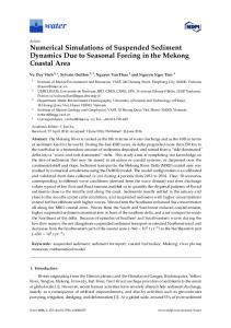
A series of experiments for water wave generation by a solid body plunger 共Scott Russell wave generator兲 has been conducted at LIAM laboratory, L’Aquila University, Italy 共Di Risio 2005兲. The experiments were performed in a three-dimensional flume 12 m long, 0.45 m deep, and 0.3 m wide 共see Fig. 1兲. Rectangular cylinders with width= 0.3 m 共same as flume兲, height= 0.1 m 共vertical direction兲, and variable length 共in flume direction, see Table 1 and Fig. 1兲 are released vertically at one end of the flume to generate waves. The space between the cylinder and the vertical walls of the flume is less than 1 mm. The specific weight of the cylinder is 1.33 t / m3. Three lengths of rectangular rigid body 共0.05, 0.1, and 0.15 m兲 are used. Twenty one tests were conducted 共see Table 1兲. Three different initial elevations of the cylinder are tested: partially submerged 共the bottom of the cylinder is 3 cm below the still water level兲; on the still water level; and aerial 共3 cm above the still water level兲. The water depth in the flume is also varied: 6, 10, 18, and 23 cm. Among these tests, three representative cases 共L10H10M3, L10H10P3, and L10H18P3兲 are discussed in this paper. During the experiments, five wave gauges are installed along the flume to measure the free surface elevation. A digital video camera 共Canon XM1兲 with a frame acquisition rate of 25 Hz is used to record the wave profile in the generation region.
204 205 206 207 208 209 210 211 212 213 214 215 216 217 218 219 220 221 222 223 224 225 226
Numerical Results
227
The free falling rectangular body and the subsequent wave generation and propagation are modeled in the two-dimensional 共2D兲 vertical plane. For the RANS model, a computational domain of 1.4 m ⫻ 0.4 m is discretized with uniform grid size of 0.5 cm in horizontal direction and 0.25 cm in vertical direction. A rectangular shape rigid body is placed at the left end of the domain at a given height relative to the still water free-surface level and allows falling under gravity. Free-slip boundary conditions are applied on all the boundaries except at the right end of the computational domain, where the radiation boundary condition is imposed so as to ensure outgoing waves through the boundary. The same k-⑀ model is used for the boundary layer on the solid boundary including a vertical plunger. In the numerical simulations, it is assumed that there is no space between the rigid boundary of the falling cylinder and the left boundary of the computational domain and the motion of falling body is always in perfectly vertical direction without rotation. The frictional forces acting on the surfaces of the box that are in contact with the vertical wall of the flume are assumed to be proportional to the contact area of the body with the wall, i.e., larger frictional forces are used for the box with larger dimension. The dynamic coefficient of friction used for the computation of three representative cases is = 0.66.
228 229 230 231 232 233 234 235 236 237 238 239 240 241 242 243 244 245 246 247 248 249 250
JOURNAL OF WATERWAY, PORT, COASTAL, AND OCEAN ENGINEERING © ASCE / MAY/JUNE 2008 / 3
Fig. 1. 共a兲, 共b兲 Locations of wave gauges; 共c兲 picture of 2D flume; and 共d兲 Scott Russell wave generator
251 252 253 254 255 256 257 258 259 260 261 262 263 264 265 266 267 268 269 270 271 272 273 274 275
In computing the total force on the falling cylinder, the shear stress induced by flow motions, which is applied in a tangential direction on the moving boundary, is assumed to be negligible. Thus, only the normal forces obtained by integrating pressures along the moving boundaries are considered in this study. Motion of the cylinder for the RANS model is advanced by solving dynamic equilibrium. The validity of the shear force assumption will be examined in a later section and further discussed in the “Concluding Remarks.” For the SPH model, numerical simulations have been carried out using a computational domain of 2.0 m ⫻ 0.5 m, with particle diameter equal to 0.004 m. Initially, particles have been placed on a regular grid, with uniform grid size of 0.004 m. Boundaries and the rigid box falling into water have been modeled using repellent particles 共Monaghan 1994兲, with free-slip conditions on all surfaces. In all simulations, the ␣ parameter assumed the value ␣ = 0.07. Motion of the cylinder for the SPH model is prescribed by the experimental data. No dynamic equilibrium is considered. For both RANS and SPH models, mesh regeneration is not required during the simulation. The same rectangular mesh in Cartesian coordinate is used with moving boundary condition throughout the simulation. Three-dimensional effects are observed in some of the experiments. Differences in the free-surface elevation on one side wall of tank and the other side wall were noticed. However, these 3D
effects occurred when the wave was propagating after the wave generation. It is noted that 3D effects are negligible in the wave generation region. For the numerical simulations and comparisons presented in the following sections, the Reynolds numbers ranges from 2.3e + 4 to 5.9e + 4, the Froude number from 0.22 to 0.42, and simulation step sizes range from 0.0005 to 0.005, respectively.
276
Comparisons of RANS and SPH Model Predictions
283
Three selected cases of the physical experiments are presented in this section to examine the prediction capabilities between the two numerical models. The same rigid body is employed in all three cases. However, Cases I and II have identical water depths but different initial rigid body vertical locations. In Case I, the bottom of the rigid body is initially below the still water lever 共SWL兲 whereas in Case II, the bottom of the body is above the SWL. For Case III, the bottom of the rigid body has identical initial height with respect to the SWL as in Case II. However, the body is dropped into a large water depth.
284 285 286 287 288 289 290 291 292 293
Case I In the first representative case 共referred to as Test L10H10M3兲, the rigid body with dimensions of 0.1 m ⫻ 0.3 m ⫻ 0.1 m 共length⫻ width⫻ height兲 is located initially 3 cm below the SWL
294 295 296 297
4 / JOURNAL OF WATERWAY, PORT, COASTAL, AND OCEAN ENGINEERING © ASCE / MAY/JUNE 2008
277 278 279 280 281 282
Table 1. Experiments Configurations Initial box location 共cm兲 +3
Box length 共cm兲
Water depth 共cm兲
Test
5
6 10 6 10 18 23 6
L5H6P3 L5H10P3 L10H6P3 L10H10P3 L10H18P3 L10H23P3 L15H6P3
6 6 10 18 23 6
L5H6M3 L10H6M3 L10H10M3 L10H18M3 L10H23M3 L15H6M3
6 10 18 6 10 18 23 6
L5H6PM0 L5H10PM0 L5H18PM0 L10H6PM0 L10H10PM0 L10H18PM0 L10H23PM0 L15H6PM0
10
15 −3
5 10
15 0
5
10
15
298 and is released into the 0.1 m deep water. The time history of box 299 displacement computed based on the RANS model is compared 300 with experimental data in Fig. 2. Very good agreement is ob301 served. We remark here that the numerically simulated displace302 ment of the falling rigid body does not reach the bottom of the 303 flume. In both SPH and RANS, simulation of the rigid body mo304 tion based on dynamic equilibrium is stopped when the bottom of 305 the rigid body reaches a distance less than the particle diameter, in 306 the case of SPH, and the last computational cell height, in the 307 case of RANS, above the bottom of the flume to avoid numerical 308 instability. After this time step, consistent with the physics of the 309 experiment, the rigid body is held in place while simulation of the 310 fluid dynamic continues. This procedure is applied to simulations
for all cases examined in this paper. The numerical instability and the limitation of the model will be further discussed later in this paper. A snapshot of the free surface profile and the location of the cylinder at t = 0.32 s is also shown in Fig. 2. The numerical 共RANS兲 solutions for the locations of boundaries of the rigid body and the free surfaces are shown in thick solid lines, which are overlapped on the experimental image for direct comparisons. Again, very good agreement with experimental data is observed. The time series of the free surface elevation at x = 0.4 and 0.85 m of Test L10H10M3 for both RANS and SPH numerical predictions are shown together with the measured experimental data in Fig. 3. The generated wave is a solitary-like wave with small trailing waves. Both numerical predictions match the experimental results well, with the SPH model being slightly more dissipative, resulting in a less oscillatory motion of the free surface after the main wave has passed. The calculated maximum wave heights at both stations show good agreement with experimental data. However, a slight phase difference is observed, which could be caused by the different reference times used in the experiment measurements. Figs. 4 and 5 show the predicted pressure and velocity fields, respectively, of the RANS and SPH models at various times. While the rigid body is falling, high pressures are observed at the bottom left corner of the flume, where the velocity is diminishing, and at the same time flow separation occurs at the bottom right corner of the moving body as shown in the snapshots at t = 0.2 s of Figs. 4 and 5. Subsequently, a large counterclockwise vortex is generated in the front of the moving body 共see Fig. 5兲. The RANS model results show that the vortex is advected downstream 共positive x direction兲 with a much slower speed than the phase speed of the generated solitary-like wave. Furthermore, the SPH results indicate that the vortex is attached to the front face of the rigid body until the body reaches the bottom of the flume. This discrepancy in two numerical results needs to be further examined with velocity measurements. We also observe that the pressure near the vortex center is less than the hydrostatic pressure.
311
Case II In the second case 共Test L10H10P3兲, the rigid body size and water depth are the same as those in Case I. However, the initial elevation of the bottom of the cylinder is 3 cm above the SWL.
348
Fig. 2. Snapshot of rigid body with free surface profile at t = 0.32 s 共a兲; time history of rigid body displacement 共b兲 共Case I, Test L10H10M3兲 JOURNAL OF WATERWAY, PORT, COASTAL, AND OCEAN ENGINEERING © ASCE / MAY/JUNE 2008 / 5
312 313 314 315 316 317 318 319 320 321 322 323 324 325 326 327 328 329 330 331 332 333 334 335 336 337 338 339 340 341 342 343 344 345 346 347
349 350 351
Fig. 3. Time histories of free surface elevation at x = 0.4 and 0.85 m obtained from RANS model 共a兲; SPH model 共b兲 共Case I, Test L10H10M3兲 352 The numerical results and experimental data for the movement of 353 the falling cylinder and the snapshot of the free surface profile at 354 t = 0.32 s are shown in Fig. 6. Since the initial elevation of the 355 cylinder is above the SWL, as the cylinder impacts and enters the 356 water body, violent flow motions and free surface splashing occur. 357 As shown in Fig. 6, the RANS model predicts the free surface 358 reasonably well except that the splash height is underpredicted, 359 which could be caused by the lack of required grid resolution in 360 the numerical model. The time histories of free surface displace361 ment at x = 0.4 and 0.85 m are plotted in Fig. 7. It is clear that 362 because the initial potential energy of this case is larger than that 363 of the previous case, larger waves 共the wave height to water depth 364 ratio is about 0.4 at x = 0.4 m兲 are generated near the plunging 365 cylinder and the leading wave attenuates significantly between 366 these two wave gauge locations 共the wave height to water depth 367 ratio is reduced to 0.3 at x = 0.85 m兲. Furthermore, the amplitude 368 dispersion seems to play an important role since the width of the 369 leading wave has increased. The numerical results obtained from 370 both the RANS and SPH models show slightly faster propagation 371 speeds. As shown in Figs. 8 and 9, the influence of the falling 372 rigid body on the fluid motion is much stronger than in the pre373 vious case with an initially submerged location. The free surface 374 in the front face of the moving body is separated during the im375 pact and higher pressures near the bottom left corner of the flume 376 are observed as in the previous case.
results are in reasonably good agreement with the experimental data. Up to the point when the top of the falling rigid body is at the SWL, the pressure and velocity fields show behavior similar to those in Case II 共Figs. 12 and 13兲. However, since the water depth is larger than the height of the falling cylinder, as the cylinder moves farther downwards 共i.e., the top of cylinder becomes below the SWL兲 it is overtopped by a wave propagating towards the left end of the flume, which is then reflected back into the flume. Splashing at the end wall with strong turbulence intensity is observed 共see Figs. 12 and 13兲. Unlike in the previous two cases, the vortex generated in front of the falling cylinder remains attached throughout the entire process. Discrepancy between numerical results and the experiment data are noticeable in comparisons of the time histories of free surface elevation after t ⬇ 1.5 s 共see Fig. 11兲. While the amplitude and phase of the leading wave is predicted accurately by both models, the RANS model results show a significant phase lag at the location x = 0.4 m. On the other hand, the SPH model does not predict well the amplitude of the third and higher trailing waves at the location x = 0.4 m and the shape of the second and higher trailing waves at the location x = 0.85 m. We remark here that the random nature of the splashing fluid particles and 3D air bubbles observed in the experiments might cause these discrepancies.
383
Turbulence Intensity
406
Case III In the third case 共Test L10H18P3兲, the same size of cylinder is initially located 3 cm above the SWL and released into 0.18 m deep water, which is deeper than that in the previous two cases. The snapshot in Fig. 10 shows the position of falling rigid body and the free surface profile generated at t = 0.32 s. The numerical
A study of the turbulence behaviors induced by different falling heights and bodies 共i.e., Cases I–III兲 is presented in this section. Only results from RANS model predictions are examined here because turbulence intensity predictions from direction SPH computation and measured turbulence data are not available. Fig. 14共a兲 shows the time evolution of the turbulence intensity
407 408 409 410 411 412
377 378 379 380 381 382
6 / JOURNAL OF WATERWAY, PORT, COASTAL, AND OCEAN ENGINEERING © ASCE / MAY/JUNE 2008
384 385 386 387 388 389 390 391 392 393 394 395 396 397 398 399 400 401 402 403 404 405
Fig. 4. Contour plots of pressure field computed by RANS 共a兲; SPH 共b兲 models at t = 0.2, 0.4, 0.6, and 0.8 s 共Case I, Test L10H10M3兲
JOURNAL OF WATERWAY, PORT, COASTAL, AND OCEAN ENGINEERING © ASCE / MAY/JUNE 2008 / 7
Fig. 5. Vector plots of velocity field computed by RANS model 共a兲; SPH model 共b兲 at t = 0.2, 0.4, 0.6, and 0.8 s 共Case I, Test L10H10M3兲
8 / JOURNAL OF WATERWAY, PORT, COASTAL, AND OCEAN ENGINEERING © ASCE / MAY/JUNE 2008
Fig. 6. Snapshot of position of rigid body and free surface profile at t = 0.32 s 共a兲; displacement time history of moving rigid body 共b兲 共Case II, Test L10H10P3兲 413 for Case I. Note that, for the initially submerged bottom drop, 414 turbulence is generated at the bottom surface as the fluid below 415 the falling rigid body is being pushed aside and a vortex is formed 416 共where the turbulence intensity is the highest兲 at the sharp corner 417 as expected. Based on an examination of the numerical data 共not 418 shown here due to space limitation兲 the turbulence intensity in419 creases as the rigid block continues to fall, and as shown in the 420 figure, the vortex becomes detached from the rigid body once its 421 motion stopped. The vortex then attaches to the bottom boundary
and propagates downstream with the surface wave created. The turbulence intensity decreases as the vortex moves further downstream due to energy dissipation. In Case II, because of the higher initial elevation and in air acceleration of the body, the maximum pressure and turbulence intensity obtained were higher than the initially submerged rigid body drop test of Case I as anticipated. In fact, as shown in Fig. 14共b兲, in addition to the turbulence intensity generated at the rigid body bottom surface, higher turbulence intensity also occurs at
Fig. 7. Experimental data and numerical results 关RANS model in 共a兲; SPH model in 共b兲兴 for time histories of free surface elevation at x = 0.4 and 0.85 m 共Case II, Test L10H10P3兲 JOURNAL OF WATERWAY, PORT, COASTAL, AND OCEAN ENGINEERING © ASCE / MAY/JUNE 2008 / 9
422 423 424 425 426 427 428 429 430
Fig. 8. Contour plot of pressure field computed by RANS 共a兲; SPH 共b兲 at t = 0.2, 0.4, 0.6, and 0.8 s 共Case II, Test L10H10P3兲
10 / JOURNAL OF WATERWAY, PORT, COASTAL, AND OCEAN ENGINEERING © ASCE / MAY/JUNE 2008
Fig. 9. Vector plot of velocity field computed by RANS 共a兲 model; SPH 共b兲, model at t = 0.2, 0.4, 0.6, and 0.8 s 共Case II, Test L10H10P3兲
JOURNAL OF WATERWAY, PORT, COASTAL, AND OCEAN ENGINEERING © ASCE / MAY/JUNE 2008 / 11
Fig. 10. Snapshot of position of rigid body and free surface profile at t = 0.32 s 共a兲; displacement time history of moving rigid body 共b兲 共Case III, Test L10H18P3兲 431 the free surface of the wave, which is separated from the vertical 432 body surface on the right hand side. After the falling motion of 433 the rigid body has ceased, the vortex generated at the sharp corner 434 propagates downstream as in Case I discussed above. By the time 435 t = 0.8 s, the vortex has not traveled as far downstream as that in 436 Case I and turbulence at the rigid body surface still persists. Fig. 14共c兲 shows the time evolution of the turbulence intensity 437 438 of the fluid in the vicinity of the falling rigid body for Case III. As 439 expected, the initial fluid flow and turbulence behavior for this 440 case are identical to that of Case II because of identical body and 441 initial elevation with respect to the SWL 关see top diagrams of 442 Figs. 14共b and c兲, t = 0.2 s兴, and fluid motion has not yet propa-
gated to the bottom of the shallower depth, thus the difference in bottom boundary conditions 共different depths兲 has no influence on the flow. The flow and turbulence behaviors of Case III begins to differ from those of Case II when the influence of the bottom boundary of Case II becomes noticeable, as shown in t = 0.4 s in Figs. 14共b and c兲. At this time, the motion of the rigid body in Case II has stopped and the vortex at the sharp corner begins to propagate downstream. However, for Case III, the rigid body is still falling and the fluid originally displaced by the falling body returned over the top of the body with high turbulence intensity. As the rigid body continues to fall to a large depth, the vortex
Fig. 11. Contour plot of pressure field computed by RANS model 共a兲; SPH model 共b兲 at t = 0.2, 0.4, 0.6, and 0.8 s 共Case III, Test L10H18P3兲 12 / JOURNAL OF WATERWAY, PORT, COASTAL, AND OCEAN ENGINEERING © ASCE / MAY/JUNE 2008
443 444 445 446 447 448 449 450 451 452 453
Fig. 12. Vector plot of velocity field computed by RANS model 共a兲; SPH model 共b兲 at t = 0.2, 0.4, 0.6, and 0.8 s 共Case III, Test L10H18P3兲
JOURNAL OF WATERWAY, PORT, COASTAL, AND OCEAN ENGINEERING © ASCE / MAY/JUNE 2008 / 13
Fig. 13. Experimental data and numerical results 关RANS model in 共a兲; SPH model in 共b兲兴 for time histories of free surface elevation at x = 0.4 and 0.85 m 共Case III, Test L10H18P3兲
14 / JOURNAL OF WATERWAY, PORT, COASTAL, AND OCEAN ENGINEERING © ASCE / MAY/JUNE 2008
Fig. 14. Turbulence intensity 共m/s兲 computed by the RANS model at t = 0.2, 0.4, 0.6, and 0.8 seconds: 共a兲 Case I, Test L10H10M3; 共b兲 Case II, Test L10H10P3; and Case III, Test L10H18P3 共note the vertical and horizontal scales are different for the three cases
JOURNAL OF WATERWAY, PORT, COASTAL, AND OCEAN ENGINEERING © ASCE / MAY/JUNE 2008 / 15
454 generated at the sharp edge continues to intensify and thus has the 455 highest strength among the three cases 关see Fig. 14共c兲 for t = 06 456 and 0.8 s兴. Note that energy dissipation can be observed in all three cases 457 458 when the body motion has ceased and the vortex leaves the edge 459 and begins to propagate downstream. We want to point out that a 460 validation of the turbulence intensity model capability cannot be 461 provided in this study because of the lack of experimental veloc462 ity field data. It is recommended that a velocity measurement 463 device capable of capturing the details of the velocity fields be 464 employed in a future study so that the accuracy and validity of 465 numerical results can be examined more thoroughly. 466 Relative Magnitude of Shear and Pressure Forces on 467 Rigid Body 468 469 470 471 472 473 474 475 476 477 478 479 480 481 482 483
Finally, to determine the validity of the assumption that the shear forces on the rigid body surfaces are negligible, the ratio between the shear stress and the corresponding normal stress on the top, front, and bottom surfaces of the rigid body are computed from the RANS model for the three test cases at several time intervals. As a typical example, for Case III 共Test L10H18P3兲 at t = 0.4 s, we found that the shear to normal force ratios on the top, front, and bottom surfaces of the moving rigid body are 共0.057N / 26.578N兲 0.21%, 共0.554N / 78.567N兲 0.71%, and 共0.393N / 155.960N兲 0.25%, respectively. We noted that in general, the ratio of shear to normal force at each face is less than 1% throughout the simulation period, thus validating the assumption. Because there is no experimental measurement of pressure and forces available to determine the accuracy of the numerical predictions, it is not fruitful to compare RANS and SPH numerical pressure and shear force predictions against each other.
484
Concluding Remarks
485 486 487 488 489 490 491 492 493 494 495 496 497 498 499 500 501 502
Two 2D numerical models—the RANS with a VOF free-surface capturing method and the SPH—have been presented. The capability and accuracy of these models are validated by comparing numerical results with experimental data involving wave generation by dropping a rigid body at various heights into a 2D flume partially filled with water 共Scott Russell wave generator兲. In general, the numerical results from both models are in good agreement with experimental data in terms of the displacement time history of the falling cylinder and the free surface elevation time series. The RANS model appears to be able to better predict the amplitude and phase of the trailing waves than the SPH model. The SPH model consistently predicts higher dissipation of these waves at given fixed locations. The differences in the velocity field between the two models are significant. This could be the result of different numerical resolution employed in these models. We recommend that more detailed experimental measurements of the velocity field be collected in a future study to further validate the numerical models.
503
Acknowledgments
504 505 506 507
Partial support from the National Science Foundation Grant Nos. CMS-9908392 and CMS-0217744, and the U.S. Office of Naval Research Grant Nos. N00014-04-10008 and N00014-06-10326 are gratefully acknowledged. Experiments and the SPH numerical
simulations were funded by The Italian National Dam Office and by MIUR projects 共COFIN 2004 “Onde di maremoto generate da frane in corpi idrici: meccanica della generazione e della propagazione, sviluppo di modelli previsionali e di sistemi di allerta in tempo reale basati su misure mareografiche”兲 whose scientific coordinator is Professor Paolo De Girolamo, L’Aquila University. He is gratefully acknowledged. Finally, the writers thank the Consorzio Ricerca Gran Sasso that has provided the computer resources needed to run SPH simulations.
508
References
517
Belytschko, T., Liu, W. K., and Moran, B. 共2000兲. Nonlinear finite element for continua and structures, Wiley, West Sussex, U.K. Chang, K-A., Hsu, T.-J., and Liu, P. L.-F. 共2001兲. “Vortex generation and evolution in water waves propagating over a submerged rectangular obstacle. Part I. solitary waves.” Coastal Eng., 44, 13–36. Chang, K. A., Hsu, T.-J., and Liu, P. L.-F. 共2005兲. “Vortex generation and evolution in water waves propagating over a submerged rectangular obstacle. Part II: Cnoidal waves.” Coastal Eng., 52共3兲, 257–283. Chorin, A. J. 共1968兲. “Numerical solution of the Navier-Stokes equations.” Math. Comput., 22, 745–762. Di Risio, M. 共2005兲. “Landslide generated impulsive waves: Generation, propagation and interaction with plane slopes.” Ph.D. thesis, Univ. Degli Studi di Roma Tre, Rome. Gingold, R. A., and Monaghan, J. J. 共1977兲. “Smoothed particle hydrodynamics: Theory and application to non-spherical stars.” Mon. Not. R. Astron. Soc., 181, 375–389. Hirt, C. W., and Nichols, B. D. 共1981兲. “Volume of fluid 共VOF兲 method for the dynamics of free boundaries.” J. Comput. Phys., 39, 201–225. Hsu, T.-J., Sakakiyama, T., and Liu, P. L.-F. 共2002兲. “A numerical model for waves and turbulence flow in front of a composite breakwater.” Coastal Eng., 46, 25–50. Johnson, G. R., Stryk, R. A., and Beissel, S. R. 共1996兲. “SPH for high velocity impact computations.” Comput. Methods Appl. Mech. Eng., 139, 344–373. Lin, P. 共1998兲. “Numerical modeling of breaking waves.” Ph.D. thesis, Cornell Univ., Ithaca, N.Y. Lin, P., and Liu, P. L.-F. 共1998a兲. “A numerical study of breaking waves in the surf zone.” J. Fluid Mech., 359, 239–264. Lin, P., and Liu, P. L.-F. 共1998b兲. “Turbulence transport, vorticity dynamics, and solute mixing under plunging breaking waves in surf zone.” J. Geophys. Res., 103, 15677–15694. Liu, P. L.-F., and Al-Banaa, K. 共2004兲. “Solitary wave runup and force on a vertical barrier.” J. Fluid Mech., 505, 225–233. Liu, P. L.-F., Lin, P., Chang, K.-A., and Sakakiyama, T. 共1999兲. “Numerical modeling of wave interaction with porous structures.” J. Waterway, Port, Coastal, Ocean Eng., 125共6兲, 322–330. Lucy, L. B. 共1977兲. “Numerical approach to testing the fission hypothesis.” Astron. J., 82, 1013–1024. Monaghan, J. 共1994兲. “Simulating free surface flows with SPH.” J. Comput. Phys., 110, 399–406. Monaghan, J., and Kos, A. 共2000兲. “Scott Russell’s wave generator.” Phys. Fluids, 12, 622–630. Monaghan, J., Kos, A., and Issa, N. 共2003兲. “Fluid motion generated by impact.” J. Waterway, Port, Coastal, Ocean Eng., 129共6兲, 250–259. Morris, J. 共1996兲. “Analysis of smoothed particle hydrodynamics with applications.” Ph.D. thesis, Monash Univ., Melbourne, Australia. Panizzo, A. 共2004a兲. “Physical and numerical modeling of subaerial landslide generated waves.” Ph.D. thesis, Univ. degli studi di L’Aquila, L’Aquila, Italy. Panizzo, A. 共2004b兲. “SPH modelling of water waves generated by landslides.” Proc., Convegno di Idraulica e Costruzioni Idrauliche IDRA 2004, Trento, Italy. Panizzo, A., and Dalrymple, R. A. 共2004兲. “SPH modelling of underwater
518 519 520 521 522 523 524 525 526 527 528 529 530 531 532 533 534 535 536 537 538 539 540 541 542 543 544 545 546 547 548 549 550 551 552 553 554 555 556 557 558 559 560 561 562 563 564 565 566 567 568 569 570
16 / JOURNAL OF WATERWAY, PORT, COASTAL, AND OCEAN ENGINEERING © ASCE / MAY/JUNE 2008
509 510 511 512 513 514 515 516
571 572 573 574 575 576
landslide generated waves.” Proc. ICCE 2004, Lisbon, Portugal. Rodi, W. 共1980兲. Turbulence models and their application in hydraulics—A state-of-the-art review, IAHR. Schlatter, B. 共1999兲. “A pedagogical tool using smoothed particle hydrodynamics to model fluid flow past a system of cylinders.” Ph.D. thesis, Dual MS Project, Oregon State Univ., Corvallis, Ore.
Shih, T. H., Zhu, J., and Lumley, J. L. 共1996兲. “Calculation of wallbounded complex flows and free shear flows.” Int. J. Numer. Methods Fluids, 23, 1133–1144. Yuk, D., Yim, S. C., and Liu, P. L. F. 共2006兲. “Numerical modeling of submarine mass-movement generated waves using RANS model.” Comput. Geosci., 32, 927–935.
JOURNAL OF WATERWAY, PORT, COASTAL, AND OCEAN ENGINEERING © ASCE / MAY/JUNE 2008 / 17
577 578 579 580 581 582