Text Classification by Aggregation of SVD

Text Classification by Aggregation of SVD Eigenvectors Panagiotis Symeonidis and Ivaylo Kehayov and Yannis Manolopoulos Aristotle University, Department of Informatics, Thessaloniki 54124, Greece {symeon, kehayov, manolopo}@csd.auth.gr

Abstract. Text classification is a process where documents are categorized usually by topic, place, readability easiness, etc. For text classification by topic, a well-known method is Singular Value Decomposition. For text classification by readability, “Flesh Reading Ease index” calculates the readability easiness level of a document (e.g. easy, medium, advanced). In this paper, we propose Singular Value Decomposition combined either with cosine similarity or with Aggregated Similarity Matrices to categorize documents by readability easiness and by topic. We experimentally compare both methods with Flesh Reading Ease index, and the vector-based cosine similarity method on a synthetic and a real data set (Reuters-21578). Both methods clearly outperform all other comparison partners.

1

Introduction

Data mining algorithms process large amount of data to find interesting patterns from which useful conclusions can be extracted. Several popular data mining techniques (Naive Bayes classifier, TF/IDF weights, Latent Semantic Indexing, Support Vector Machines etc.) have been used for text categorization. Most of them are based on the vector space model for representing documents as vectors. These methods categorize documents by topic, place or people interests. In this paper, we are interested in categorizing documents by readability easiness. In particular, we exploit the vector space model for representing documents. Then, we use Singular Value Decomposition (SVD) for dimensionality reduction to categorize documents by readability easiness. Our advantage over other methods relies on the fact that SVD reduces noise, which is critical for accurate text categorization. In addition, we propose a new method, denoted as Aggregated SVD, which creates distance matrices that contain distances/dissimilarities between documents. These distance matrices are combined using an aggregation function, creating a new distance/dissimilarity matrix. As will be experimentally shown, this aggregated new matrix boosts text categorization accuracy. The contribution of this paper is two-sided: Firstly, it proposes a new text categorization technique (Aggregated SVD). Secondly, it compares the accuracy performance of several methods for text categorization by readability easiness. The rest of the paper is structured as follows. In Section 2, we present the related work. In Section 3, we present basic information for text categorization by

readability easiness. In Section 4, we present how classic SVD is applied in text categorization. In Section 5, we describe our new proposed method, denoted as Aggregated SVD. Experimental results are presented in Section 6. Finally, Section 8 concludes this paper.

2

Related work

The application of SVD in a document-term vector space model has been proposed in [FD88] in the research area of information retrieval. Documents and queries are represented with vectors and SVD is applied for reducing the dimensions of these vectors. Yang Yu [Y97] published a comparative evaluation of twelve statistical approaches to text categorization. Moreover, Joachims [J98] explored the usage of Support Vector Machines for learning text classifiers and identified the benefits of SVMs for text categorization. Sarwar et al. [SKKR00] compared experimentally the accuracy of a recommender system that applies SVD on data with the one that applies only collaborative filtering. Their results suggested that SVD can boost the accuracy of a recommender system. Panagiotis Symeonidis [S07] applied Latent Semantic Indexing (LSI) on feature profiles of users of a recommender system. These feature profiles are constructed by combining collaborative with content features. Dimensionality reduction is applied on these profiles by using SVD, to achieve more accurate item recommendations to users. Guan et al. [GZG09] proposed Class-Feature-Centroid classifier for text categorization, denoted as CFC classifier. It adopts the vector space model and differs from other approaches in how term weights are derived, by using inner-class and inter-class term indices. Hans-Henning et al. [HSN10] proposed a method that creates self-similarity matrices from the top few eigenvectors calculated by SVD. Then, these matrices are aggregated into a new matrix by applying an aggregating function. Our method differentiates from their work as follows. Their method has been used for boosting clustering of high dimensional data. In contrast, we are exploiting Aggregated SVD for text categorization purposes.

3

Preliminaries in Text Categorization by readability easiness

In this Section, we provide the basic methodology, which is usually followed for text categorization by readability easiness. More specifically, we divide documents to a training and a test set. Then, we compare each document that belongs to the test set to each document that belongs in the training set and decide in which category by readability easiness (easy, medium, advanced) it belongs. To compare one document to another the documents must be represented by vectors. The vectors of all documents have the same length which is the length of

the dictionary. The dictionary is a vector that contains all the unique words of all documents in the training set. The value of each dimension in a document’s vector is the frequency of a specific word in that document. For example, the value of the fifth dimension in a document’s vector is the appearance frequency of the word of the dictionary’s fifth dimension. The words are also called terms, the dimensions’ values are called term frequencies and the documents’ vectors are called frequency vectors. In the following, we present how vector space model is applied in the following three documents: D1: Sun is a star. D2: Earth is a planet. D3: Earth is smaller than the Sun. The dictionary is the vector: Dictionary = [a, Earth, is, planet, smaller, star, Sun, than, the] As we can see, the length of the vector is 9. The frequency vectors of the three documents are: D1 = [1, 0, 1, 0, 0, 1, 1, 0, 0] D2 = [1, 1, 1, 1, 0, 0, 0, 0, 0] D3 = [0, 1, 1, 0, 1, 0, 1, 1, 1] Frequency values are either 0 or 1 because documents are very small. Some terms, like “a” and “is”, are found in every document or in the majority of them. These terms do not offer any useful information that helps the document categorization and are considered as noise. If we can remove them somehow then the categorization will be done more effectively. For this purpose, stop words can be used, which is a list of words that will be ignored during the creation of the dictionary and the frequency vectors. Instead of using stop words, we remove most of the noise by dimensionality reduction of the frequency vectors through SVD (Singular Value Decomposition). A method that is widely used and does not belong to the field of data mining is Flesh Reading Ease index. It is based on three factors: (i) total number of syllables (ii) total number of words and (iii) total number of sentences in the document. Based on these three factors, Flesh Reading Ease index calculates a score from 0 to 100 for each document. The higher the score the easier the document is to be read. The formula for the English language is as follows:     totalsyllabes totalwords − 84.6 (1) 206.835 − 1.015 totalsentences totalwords As we can see, more syllables per word as well as more words per sentence mean higher reading difficulty and vice versa.

Table 1. Explanation of Flesh Reading Ease Score. Score Readability Level 71-100 Easy 41-70 Medium 0-40 Advanced

Notice that we categorize documents by their reading easiness into three categories: easy, medium and advanced. Table 1 shows how the Flesh Reading Ease score corresponds to the three categories.

4

The classic SVD method

By applying the SVD technique to a m × n matrix A, it can be analyzed to a product of three matrices: an m × m orthogonal matrix U , a m × n diagonal matrix S and the transpose of an n × n orthogonal matrix V [S07]. The SVD formula is: T Am×n = Um×m Sm×n Vn×n

(2) T

The columns of U are orthonormal eigenvectors of AA , S is a diagonal matrix containing the square roots of eigenvalues from U or V in descending order and the columns of V are orthonormal eigenvectors of AT A. To remove some noise from the data, dimensionality reduction should be applied. This is done by removing rows from the bottom of matrices U and S and left columns from matrices S and V T . Next, we will use SVD to categorize documents by readability easiness with a running toy example. We categorize the documents into three categories: easy, medium and advanced. Table 2 contains the document frequency vectors of the training set. Each row of the table is a frequency vector. There are 9 documents and 10 unique terms. The first three documents (D1-D3) belong to the category easy, the next three (D4-D6) to category medium and the last three (D7-D9) to category advanced. The length of the dictionary and therefore of the vectors is 10 due to the number of the unique terms. The first three terms (T1-T3) have higher frequency values in the first three documents because these terms define the category easy. For the same reason, the second three terms (T4-T6) define the category medium and the next three (T7-T9) the category advanced. The last term (T10) does not describe any category and is considered as noise. We apply SVD on the data of Table 2: T S9×10 = U9×9 S9×10 V10×10

(3)

Let’s assume that we insert a new document in our systems (i.e. test set): test = [4, 4, 5, 3, 2, 2, 0, 3, 0, 1]

(4)

Table 2. Frequency vectors of the documents.

D1 D2 D3 D4 D5 D6 D7 D8 D9

T1 4 5 2 2 1 3 0 2 1

T2 6 5 3 2 0 2 0 3 1

T3 2 3 4 3 1 0 2 3 0

T4 3 1 0 5 2 5 3 0 3

T5 3 1 0 6 3 6 2 0 3

T6 1 2 0 4 2 5 3 3 2

T7 1 3 2 3 2 4 5 5 4

T8 1 3 1 2 0 3 4 5 3

T9 0 2 2 1 2 0 6 4 3

T10 1 1 0 0 1 0 1 0 1

The document test belongs to category easy and this can be confirmed by the first three dimensions of the vector which have the highest values. To find out, in which category will SVD assign the new document, it should be compared with all the documents of the training set. But, before that, the test document should be represented in the new dimensional space. We call it test new and is calculated using matrix V and the inverse of S: −1 test new1×9 = test1×10 ∗ V10×9 ∗ S9×9

(5)

Next, the new vector test new is compared to the 9 documents of the training set and more specifically it is compared to every row of matrix U using cosine similarity. The first vector (row) of matrix U corresponds to document D1, the second to document D2, etc. The calculated cosine similarities are shown in Table 3. Table 3. Similarity of document test with the nine documents (before removing noise).

Document D1 D2 D3 D4 D5 D6 D7 D8 D9

Similarity with document test -0.14 0.53 -0.33 0.57 -0.32 -0.38 0.02 -0.13 0.03

Based on Table 3, the test document is most similar with D4, which belongs to the second category. The categorization is not right as the document test belongs to the first category. The result could be improved by using the majority vote

which takes into account the three or the five best similarities. However, in our running example, if we take the majority vote from the three best similarities (D2, D4 and D9), the text categorization result is also wrong. Up to this point, we have applied SVD but have not really taken advantage of it because we have kept all the information of the original matrix (contains noise). As we stated earlier, noise removal can be performed by dimensionality reduction [S07]. Next, we keep 80% of the total matrix information (i.e. 80% of the total sum of the diagonal of matrix S). As a result, 6 rows from the bottom of matrices U and S and 6 left columns from matrices S and V T are removed. Now, we repeat the same process as before starting with calculating the new vector for the test document: −1 test new21×3 = test1×10 ∗ V10×3 ∗ S3×3

(6)

Now, test new2 has fewer dimensions. Next, we recalculate the cosine similarity of the test document with the nine documents using the new vector. The new similarities are shown in Table 4. As shown, the categorization is now correct. The test document is most similar with D1, which belongs to the same category i.e. easy. Also, the three best similarities are with D1, D2 and D3. All three of them belong to the category easy just as the test document. That is, the 20% of information that we took away from the original matrix was actually noise. Table 4. Similarity of document test with the nine documents (after removing noise).

Document D1 D2 D3 D4 D5 D6 D7 D8 D9

5

Similarity with document test 0.97 0.87 0.69 0.37 -0.8 0.26 -0.67 0.2 -0.16

The Aggregated SVD method

In this Section, we adjust the aggregated SVD [HSN10] method, which is initially proposed for clustering of data, to run for text categorization. Clustering of high dimensional data is often performed by applying SVD on the original data space and by building clusters from the derived eigenvectors. Hans-Henning et al. [HSN10] proposed a method that combines the self-similarity matrices of

the top few eigenvectors in such a way that data are well-clustered. We extend this work by also applying SVD to a matrix that contains document frequency i vectors. Then, a distance matrix Dm×m is produced from every column of matrix Um×m . It is called distance matrix because it contains the distances (i.e. the dissimilarities) from every value of the column to the rest values of the same column. If matrix Um×m has m columns then the total distance matrices are m (i=m). Every matrix D is symmetrical and its diagonal is consisted of zeros. The values of each distance matrix are normalized as follows: x , xnormalized = p 2 2 (x1 + x2 + ... + x2N )

(7)

where x is the value normalized and {x1 , x2 , ..., xN } the values of the distance matrix that is being normalized. When all selected distance matrices are computed and normalized, they are aggregated into a new matrix M with an aggregation function. Such functions are minimum value, maximum value, average, median and sum. In our running example, we used the sum function. That is, a cell in matrix M is the sum of the values in the corresponding cells of all distance matrices. Thus, M is a symmetric matrix (after all distance matrices are symmetrical) that shows the distances between documents taking into account all columns of U . When a document is to be categorized, the same steps are followed as described in the previous section (with or without dimensionality reduction). Next, we will perform aggregated SVD on our running example. If we apply SVD on the original frequency matrix and keep 80% of the information, then matrix U remains with 3 columns. Based on these 3 columns, we can build 3 i distance matrices D9×9 (i = 1, 2, 3). By aggregating the 3 matrices we conclude with matrix M of Table 5. As we mentioned before, M is symmetric and there are only zeros on its diagonal. As far as the rest values is concerned, the closest a value is to 0 the smallest the distance of the two documents is (i.e. more similar). Table 5. Aggregation distance matrix M. The smaller value is better.

D1 D2 D3 D4 D5 D6 D7 D8 D9

D1 0 -0.7169 0.0412 0.1885 -0.0123 0.5678 0.7600 0.5862 -0.5465

D2 -0.7169 0 -0.7048 0.0978 0.6455 0.4771 -0.0737 -0.9082 -0.0440

D3 0.0412 -0.7048 0 1.0129 -0.5747 1.3922 0.8414 -0.1216 0.2780

D4 0.1885 0.0978 1.0129 0 -0.0035 -1.8320 0.1911 0.1983 -0.3611

D5 -0.0123 0.6455 -0.5747 -0.0035 0 0.2802 0.4123 0.2385 -1.0267

D6 0.5678 0.4771 1.3922 -1.8320 0.2802 0 0.4747 0.4820 -0.0774

D7 0.7600 -0.0737 0.8414 0.1911 0.4123 0.4747 0 -0.7662 -0.7722

D8 0.5862 -0.9082 -0.1216 0.1983 0.2385 0.4820 -0.7662 0 -0.6238

D9 -0.5465 -0.0440 0.2780 -0.3611 -1.0267 -0.0774 -0.7722 -0.6238 0

Next, we will categorize again the test document based on the aggregated SVD method. As previously shown in Table 4, the test document presents the

highest similarity with document D1. However, if we want to apply aggregated SVD we have to use the majority vote from two more similar documents. Based on matrix M of Table 5, these documents correspond to D3 and D5 (with values 0.0412 and -0.0123 respectively). Since documents D1-D3 belong to category easy and documents D4-D6 belong to category medium, we have two documents from category easy and one from category medium. That is, the test document is again correctly assigned to category easy.

6

Experimental Evaluation

In this Section, we experimentally compare the accuracy performance of four different methods for text categorization. These methods are: (i) k Nearest Neighbor Collaborative Filtering algorithm, denoted as Cosine, (ii) Latent Semantic Indexing, denoted as SVD, (iii) the aggregation of similarity matrices of SVDeigenvectors method, denoted as AggSVD, and (iv) the Flesh Reading Ease index, denoted as Flesh. For SVD and AggSVD, we have run experiments with different levels of dimensionality reduction. These levels are three and the information we keep in each level is 30%, 70% and 100% for each method, respectively. The last one (100%) means there is no reduction at all. The performance measures are computed as follows [Y97]: ( a , if a+b > 0 (8) P recision = a+b undefined, otherwise ( a , if a+c > 0 Recall = a+c (9) undefined, otherwise Recall ∗ P recision (10) Recall + P recision where a is the number of correctly assigned documents in a category, b is the number of incorrectly assigned documents in a category, and c is the number of documents that incorrectly have not been assigned in a category. F =2∗

7

Data Sets

To evaluate the examined algorithms, we have used a synthetic and a real data set. 7.1

Synthetic Data Set

As far as the synthetic data set is concerned, we have created an English text generator. Based on our generator, we have generated documents of the three readability categories (easy, medium and advanced) by adding also up to 50% controllable noise to each document. Our generator uses three text files (easy.txt,

medium.txt and advanced.txt) which contain terms used for generating documents. The names of the files indicate the difficulty level of the terms inside (easy.txt contains low difficulty terms, medium.txt contains medium difficulty terms and advanced.txt contains advanced difficulty terms). The generator has three input parameters: (i) number of files per category to be generated, (ii) number of terms per file to be generated and (iii) the amount of noise to be generated. For the first parameter, if the user inserts value 200 then 600 files will be generated, 200 for each category. For the last noise parameter, it is determined as a 1/x fraction. The user’s input replaces the x in the fraction. For example, if user gives value 5 then the noise will be 1/5 which is 20%. As noise the generator uses terms from the other two categories (i.e. if noise is 20% then 80% of the terms of an easy level document will be derived from easy.txt and 20% from medium.txt and advanced.txt). Additionally, punctuation is added in the documents in order to use them for evaluating Flesh method. Recall that the number of sentences is a parameter for the calculation of the Flesh score. In the first category there is a 1/10 (10%) chance of adding a dot after each term. The result is sentences with average of 10 terms. In medium category this probability is 1/15 (6.67%) or 15 terms per sentence average. In the last category this number is 1/20 (20%). As we can see, the higher the difficulty level of the text the lower the chance of dot appearance, because longer sentences mean lower readability easiness. For our experiments, we have created 1200 documents (400 documents belong to each category) in the training set and 450 documents (150 documents belong to each category) in the test set. We have also created synthetic data set versions with different noise levels (i.e. 0%, 25%, 50%, and 75%). In this work, we present only experiments with 50% controllable noise. Notice that our findings have been confirmed also to the other synthetic data set versions. 7.2

Reuters 21578 Real Data Set

As far as the real data set is concerned, we have used the Reuters 21578 corpus. Reuters 21578 collection consists of 21578 news articles published during 1987 by Reuters news agency established in London, UK. In the Reuters data set the documents are categorized by topic. There are five topic super-sets: exchanges, orgs, people, places and topics. All topics in each of these sets are content related. For each document, a human indexer decided to which topic a document belongs. Table 6 shows the topic distribution across the five sets. The topics category of Table 6 concerns economic subjects. For instance, it includes subtopics such as coconut, gold, inventories, and money −supply. Typically a document assigned to a category from one of these sets explicitly includes some form of the category name in the document’s text. However, these proper name categories are not as simple to assign correctly as might be thought. Notice that Flesh Reading Ease index was not tested with the real data set, because it calculates readability easiness score and it is not suitable for categorization by topic.

Table 6. Topic distribution of the Reuters 21578 collection.

Category Set exchanges orgs people places topics

7.3

Number of sub-Categories 39 56 267 175 135

Algorithms’ Accuracy Comparison on the Synthetic Data Set

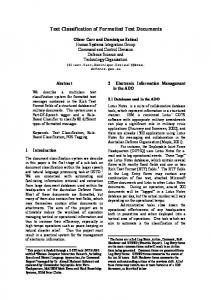
In this Section, we test all four methods’ accuracy performance on a synthetic data set with 50% controllable noise. That is, a 50% of the total document terms belong to the correct category of the document and the other 50% are terms that belong to the other two categories. Figure 1 shows the results for each readability easiness category (easy, medium, advanced ). For the documents that belong to category easy, SVD 30% has the best performance (up to 98% accuracy), followed by AggSVD 30%. Notice that Flesh presents the worst performance (under 5% accuracy). This can be explained due to the existence of high percentage of controllable noise in the data set. That is, when the noise is set up to 50%, then half of the terms have many syllables. By increasing the number of the syllables, Flesh assigns false documents to the medium or advanced category, reducing its accuracy performance. For the documents that belong to category medium, SVD 70% presents the best accuracy performance. Both AggSVD 30% and Cosine Similarity perform quite well. Notice that Flesh’s performance is substantially increased for this category. For the documents that belong to category advanced, both cosine similarity and SVD 70% perform very well. We proceed with the comparison of all four algorithms, in terms of precision and recall. This reveals the robustness of each algorithm in attaining high recall with minimal losses in terms of precision. As shown in Figure 2, the recall and precision vary as we increase the number of documents to be classified. SVD 30% precision value is almost 98% when we try to classify the first test document. The respective values for AggSVD 30% and Cosine are 96.2% and 93.5%. This experiment shows that SVD 30% and AggSVD 30% are more robust in categorizing correctly documents. The reason is that both of them perform dimensionality reduction, which removes noise from documents. In contrast, Cosine Similarity algorithm correlates document without removing the noise. Finally, Flesh presents the worst results, because it does not take into account noise at all. 7.4

Algorithms Accuracy Comparison of methods on the Real data set

In this Section, we test all methods on a real data (Reuters 21578 collection). We have chosen three topic sub-categories to test our categorizations, i.e. coffee,

Fig. 1. F-measure Diagram for the synthetic data set.

Fig. 2. Precision-Recall Diagram for the synthetic data set.

gold and ship. As shown in Figure 7.4, the result are in accordance with those of the synthetic data set. However, now the best accuracy performance of SVD is when we apply a 50% dimensionality reduction. Next, as shown in Figure 4, we plot a precision versus recall curve for all three algorithms. Once again, we re-confirm the same results with those of the synthetic data set.

8

Conclusion

In this paper, we compared the performance of four methods in classifying text documents by readability easiness and by topic. In particular, we tested the

Fig. 3. F-measure Diagram for the Reuters 21578 data set.

Fig. 4. Precision-Recall Diagram for the Reuters 21578 data set.

kNN collaborative filtering, the classic SVD, the Aggregated SVD and the Flesh Reading Ease index methods. We have shown that both classic SVD and Aggregated SVD techniques presented the best performance in a real and a synthetic data set. The results of the experiments showed us that dimensionality reduction improved the classification process in two ways: better results and better efficiency. Better results means that more documents are categorized correctly. Better efficiency means lower computation cost because the computation of the similarities between documents is done using vectors with fewer dimensions. As a future work, we indent to compare our method with other state-of-the-art comparison partners and more real data sets.

References [FD88] Furnas, G., Deerwester, et al. Information retrieval using a singular value decomposition model of latent semantic structure, SIGIR, pages 465-480, 1988 [GZG09] Guan, H., Zhou, J., Guo, M. A Class-Feature-Centroid Classifier for Text Categorization, WWW 2009, Madrid, pages 201-210, 2009 [HSN10] Hans-Henning, G., Spiliopoulou, M., Nanopoulos, A. Eigenvector-Based Clustering Using Aggregated Similarity Matrices, ACM SAC 10, pages 1083-1087, 2010 [J98] Joachims, T. Text categorization with support vector machines: Learning with many relevant features, Springer Verlag, pages 137-142, 1998 [SKKR00] Sarwar, B., Karypis, G., Konstan, J., Riedl, J. Application of dimensionality reduction in recommenders systems: A case study, ACM WebKDD Workshop, volume 1625, number 1, pages 285-295, 2000 [S07] Symeonidis, P. Content-based Dimensionality Reduction for Recommended System, GfKl 2007, pages 619-626, 2007 [Y97] Yang Y. An evaluation of statistical approaches to text categorization, Journal Information Retrieval, volume 1, number 1-2, pages 69-90, 1997