in quick transitions to virtual slide diagnosis, it is desired to have an effective way to understand pathologists' behaviors. All the aforementioned problems ...
TEXTURE BASED IMAGE RECOGNITION IN MICROSCOPY IMAGES OF DIFFUSE GLIOMAS WITH MULTI-CLASS GENTLE BOOSTING MECHANISM Jun Kong† , Lee Cooper† , Ashish Sharma†, Tahsin Kurc† Daniel J. Brat‡, and Joel H. Saltz† † Center ‡ Dept.
for Comprehensive Informatics, Emory University, Atlanta, GA 30322 of Pathology and Lab Medicine, Emory University, Atlanta, GA 30322
{jun.kong, lee.cooper, ashish.sharma, tkurc, dbrat, jhsaltz}@emory.edu
ABSTRACT The diagnosis of diffuse gliomas requires the careful inspection of large amounts of visual data. Identifying tissue regions that inform diagnosis is a cumbersome task for human reviewers and is a process prone to inter-reader variability. In this paper we present an automatic method for identifying critical diagnostic regions within whole-slide microscopy images of gliomas. We frame the problem of critical region identification as a texture-based content retrieval task in the sense that each image is represented by a set of texture features. Both linear and nonlinear dimensionality reduction techniques are utilized to explore the intrinsic dimensionality of the feature space where images are classified by classification and regression trees with performances improved by a newly extended multi-class gentle boosting (MCGB) mechanism. The proposed method is demonstrated on 1200 sample regions using a five-fold cross validation, achieving a 96.25% classification accuracy. Index Terms— Microscopy image processing, glioma, texture analysis, dimensionality reduction, gentle boosting 1. INTRODUCTION Diffuse gliomas are among the most common human brain tumors and are clinically devastating [1]. Their diagnosis is made by a pathologist’s visual inspection of a biopsy sample under microscope. The heterogeneous nature of gliomas requires the pathologist to examine multiple tissue regions for specific histopathological characteristics throughout the whole slide to arrive at a diagnostic conclusion. This is a laborious task given that some of the relevant tissue details are only perceivable at high optical magnification. Lack of adequate spatial reference may also bias the diagnosis process by causing a region to be mistakenly reviewed more than once, particularly when the biopsy is limited in size. Furthermore, the review of tissue samples would be facilitated with quantitative information, such as the relative amount of a definitive texture feature (or feature set) within the whole tissue domain. Additionally, as traditional pathology reviewing processes are
978-1-4244-4296-6/10/$25.00 ©2010 IEEE
457
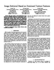
in quick transitions to virtual slide diagnosis, it is desired to have an effective way to understand pathologists’ behaviors. All the aforementioned problems motivated our development of a content-based image recognition system for digital glioma diagnosis. The proposed method intends to facilitate diagnosis by enabling pathologists to search the whole-slide microscopy image for neoplastic regions with pre-defined texture characteristics, such as glioblastoma areas coupled with necrosis and vascular hyperplasia. A comprehensive texture feature vector is used to represent each local image content. Classification and regression trees (CART) provide the means of recognition by comparing the feature vectors. To further enhance the accuracy of the CART classifier, we propose the multi-class gentle boosting (MCGB) mechanism, a novel extension of the binary gentle boosting method [2], for improving the performance of a multi-class classifier. 2. MATERIALS The database of glioma image regions used in this study consists of 1200 8-bit 256 × 256 color image tiles from four large image regions within two whole-slide microscopy images of gliomas. By visual inspections, homogeneous textures are presented within each of these four image regions. As a result, 1200 image tiles are classified into four classes, with 300 images in each category. These classes serve as the four typical cases of content that attract attentions of a pathologist during visual inspections. Representative examples of these classes are shown in Fig. 1, where examples exhibit different, though subtle, texture characteristics indicated by such image hints as cellular density and micro-anatomical structures. 3. IMAGE RECOGNITION ALGORITHM 3.1. Texture feature representation As a key component of human vision system, texture information has been found useful in diverse applications [3]. In general, textures are sophisticated perceptual patterns that follow certain spatial arrangements and have local properties [4]. Depending on the type of local characteristics to be described,
ICASSP 2010
standard deviation and the kurtosis:
σ where κ = fcon = √ 4 κ (a)
(b)
(c)
devised texture features often focus more on one group of local perceptual patterns than another. This results in the needs to use multiple texture features representing different aspects of image local properties in practice.
�I(i, j)�σ 4
(2)
3.1.3. Wavelet features The wavelet analysis can be viewed as a way to decompose images into a set of frequency channels with different spatial orientations. Given a family of basis functions {ψs,t (x)}, the wavelet decomposition of a signal S(x) can be written as: S(x) ∗ ψs,t (x) =
3.1.1. Co-occurrence matrix based features A co-occurrence matrix is defined as a second-order histogram of pairwise pixel values with respect to a given spatial relationship M (i, j)|{d, θ }, where d is the displacement distance and θ is the orientation of the spatial pairs [5]. When normalized, each entry md,θ (i, j) in the matrix becomes an estimate of the joint probability of two pixels {X1 , X2 } having co-occurring value i and j, and constrained by the spatial relationship M (i, j)|{d, θ }. As the joint distribution presented by this matrix depends on the distance and angular relationship between pairs of pixels, we set the distance constrain as d = 5, the approximate scale of the salient patterns in images. Additionally, histograms associated with eight directions from images quantized with 16 gray levels are averaged as a way to represent images invariant to rotation. To capture texture features of different natures from the co-occurrence matrix, we compute a list of features that include contrast, correlation, energy, homogeneity, entropy, dissimilarity, inverse difference moment, maximum probability [5]. 3.1.2. Tamura features Two perceptual relevant features, known as coarseness and contrast, have been largely used both in texture retrieval and content-based image retrieval systems [6]. Coarseness is a perceptual feature that aims to identify the largest scale of the structural element of texture using various neighborhood sizes. The resulting coarseness of the given image I(i, j) is the average value of all the “scales”: i
i j
where �I(i, j)� is the number of pixels in image I.
(d)
Fig. 1. Typical image examples of four image classes set up for testing the developed texture-based image recogintion method.
fcoa = ∑ ∑ σ ∗ (i, j)
∑ ∑ (I(i, j) − μ )4
� ∞ −∞
S(x)ψs,t (x) dx
(3)
where s and t are the translation and dilation parameters. With wavelet representations, the strengths of the lowfrequency channels indicate the degree of smoothness in image domains, whereas the energies in both low and middle frequencies capture the strengths of texture patterns presented in images. With a three-level wavelet decomposition, energies of ten frequency channels computed with a set of symmetric orthogonal wavelet bases[7] are used in this study. 3.1.4. Neighborhood difference matrix based features Neighborhood gray-tone difference matrix (NGRDM) is another way to extract texture features compatible with the human perception mechanism that is particularly sensitive to the spatial intensity change [8]. A vector of features that capture different perceptual clues are derived from the NGTDM. These features, including coarseness, contrast, busyness, complexity and texture strength, are used in our study with the half neighborhood size being 3 to match the scale of the most salient patterns in images (c.f. [8]). 3.1.5. Gray level run length matrix based features Gray Level Run Length Matrix (GLRLM) is a two-dimensional matrix from which higher order statistical texture features can be derived [9]. Each entry c(g, l|θ ) in GLRLM represents the number of occurrences of run-length l associated with pixels having the gray level of g along the direction θ . From the GLRLM representation with a 16 gray-level quantization, we compute 11 averaged features associated with four directions θ = {0, π4 , π2 , 34π } (c.f [9]). 3.2. Dimensionality reduction
(1)
j
As each glioma image region is represented by a vector in a high-dimensional space, we apply dimensionality reduction prior to classification to mitigate the “curse of dimensionality” and other undesired properties associated with highdimensional spaces [10]. In our experiments, we compare
where σ ∗ (i, j) is the best “scale” for pixel (i, j) (c.f.[6]). Contrast is another perceptual index that measures the dynamic range and the “peakedness” of the probability distribution of gray levels in a given image. Its value depends on the
458
linear dimensionality reduction techniques, namely Principle Component Analysis (PCA) and Linear Discriminant Analysis (LDA), with two non-linear methods, including Local Linear Embedding (LLE) [11] and Isomap[12]. Linear dimensionality reduction techniques have been used in many research work where the data distributions are assumed to be well described using linear subspaces of lower dimensions. As opposed to the traditional linear methods, it would work better for nonlinear dimensionality reduction methods to map data onto the underlying manifold with a lower dimensionality, such as the Swiss roll data set [12]. As a result, we test with both linear and non-linear methods to uncover the intrinsic feature dimensionality of our image data. 3.3. Classification with multi-class gentle boosting The classification and regression tree (CART) used in this study is a tree-graph classifier that classifies data by the most discriminating candidates selected from a large pool of variables [13]. It is organized in a binary hierarchical structure consisting of “nodes” and “leaves”, those representing some predicates and the classification results, respectively. The whole classification procedure begins from the root and follows the splitting branch indicated by the value of the current node predicate recursively until a leaf is reached. In our study, the CART classifier is designed to have maximum three splits from its root, as too many splits would inevitably invite the over-fitting problem. It is aware that CART is a weak classifier whose performance needs to be boosted with some additional performanceboosters. In this study, gentle boosting is used to improve the learning process for CART [2]. Being a more robust and stable version of the adaptive AdaBoost, gentle boosting has been formulated as an additive logistic regression fitting problem. However, gentle boosting originally can only accommodate a two-class classification problem. To fit to our needs, we extend it to solving a multi-class, i.e. four-class in this study, classification task. When combined with the CART classifier, the complete boosting algorithm for a multiclass classification problem can be described in Algorithm 1.
4. EXPERIMENTAL RESULTS We test the performances of the proposed texture-based image region recognition method using various types of dimensionality reduction techniques on the image data set comprised of 1200 images from four classes with a five-fold cross validation process. As a result, the whole data set is equally divided into five different groups across the four classes. Each time we use one of them as the training set and the remaining four as testing data. In Table. 1, we present the averages and standard deviations of the testing classification errors associated with different dimensionality reduction methods for the first
459
Algorithm 1 Gentle boosting for a multi-class problem with CART as the weak learner. Require: Given the number of class C and N pairs of data and labels: {X,Y |(xi , yi ), i = 1, 2, . . . , N} •Construct C groups of data-label pairs: {(X,Y j ) | j = 1, 2, . . . ,C} •Initialize weights wi j ← N1 , i = 1, 2, . . . , N, j = 1, 2, . . . ,C; and the voting function Fj (X) = 0 for all k = 1, 2, . . . , K iterations do for all j = 1, 2, . . . ,C do – Construct the CART classifier M kj (X,Y j ) –Fit the regression function f jk (X) = Ew j (M kj (X,Y j )|X), where Ew (Y |X) = Pw (Y = 1|X) − Pw(Y = −1|X) – Update Fj (X) ← Fj (X) + f jk (X) for all i = 1 to N do k – Update wi j ← wi j + e−yi f j (xi ) end for – Normalize wi j , ∀ i = 1, 2, . . . , N end for end for •The resulting output classification label: j∗ = arg max Fj (x)
E{w(Y )Y |X} E{w(Y )|X}
=
j={1,2,...,C}
seven boosting iterations. Of all the dimensionality reduction methods used in this study, the best performances are consistently achieved by LDA, with the best classification accuracy up to 96.25% ± 1.66%. Additionally, the classification error curve associated with LDA is decreased rapidly in our study, achieving its convergence in less than ten boosting iterations. This fact agrees with the conclusions made in [14] where it also claims the superiority of linear dimensionality reduction methods to non-linear ones for real-world data. To further investigate the reasons leading to the superior performances with LDA, we show in Fig. 2 the scatter plot of the class conditional data in the reduced dimensional space (i.e. d = 3 in this case) when LDA is used. It is apparent that the resulting data cloud of each class is relatively compact and
Table 1. The averages and the standard deviations of classification errors of the five-fold cross validation tests associated with different dimensionality reduction methods for the first seven boosting iterations are presented. Iter. 1 2 3 4 5 6 7
PCA 15.25±0.54 9.90±1.69 8.60±1.30 8.52 ± 1.08 8.40 ± 1.06 8.02 ± 1.00 8.02 ± 1.35
LDA 5.75 ± 1.60 4.15 ± 1.38 3.75 ± 1.66 3.90 ± 1.50 3.90 ± 1.57 3.81 ± 1.49 3.96 ± 1.43
LLE 20.60±5.21 10.50±1.66 10.17±0.83 10.29±0.82 10.40±1.12 9.77±0.63 10.15±1.06
ISOMAP 6.67±1.58 5.19±0.59 4.98±0.52 5.33±1.76 4.96±1.04 5.10±1.35 5.38±1.66
1
class 1 class 2 class 3 class 4
0.7522 0.7521
0.7519
0.99
0.98
0.7518
True Detection
Dimension 3
0.752
0.7517 0.7516 0.7515 0.7514 0.7536
0.97
0.96
0.7537
0.95
0.7537 0.7538
−0.7507
0.7538 −0.7509
0.7539 0.754 Dimension 1
class 1 vs. others class 2 vs. others class 3 vs. others class 4 vs. others
−0.7508 −0.7508
0.7539
0.94
−0.7509 −0.751
Dimension 2
0.93
Fig. 2. The scatter plot of the class conditional data obtained by applying LDA to the full dataset in a 3-d space. well apart from each other, which considerably contributes to a promising discrimination performance in the following classification process. With an effort on better exhibiting the method properties, we plot the Receiver Operating Characteristic (ROC) curves in Fig. 3 to further illustrate the system performance when LDA is elected. Since this is a four-class classification problem, four ROC curves are presented, each representing the ROC curve associated with one class against the other three. It is worth mentioning that the true detection rate for each curve in Fig. 3 is an average of all the five-fold testing runs. 5. CONCLUSION In this paper, we propose a fully automated method that captures regions of interest in whole-slide microscopy images of diffuse gliomas using texture information and pattern recognition techniques. The proposed method represent each image region with a family of discriminating texture features. Both linear and non-linear dimensionality reduction techniques are utilized to exploring the intrinsic dimensional feature space. With our data, LDA is found to yield the best performance. We also make a novel extension of the gentle boosting method to a multi-class mechanism for boosting the performance of the CART classifier. This method is tested on 1200 microscopy image regions of 256×256 from four texture classes. With a five-fold cross validation process, i.e. partitioning, respectively, 20% and 80% of the image regions for training and testing for each of the five validation instances, this proposed method produces an averaged accuracy of 96.25% with its standard deviation of 1.66%. 6. REFERENCES [1] D.J. Brat, R.A. Prayson, T.C. Ryken, and J.J. Olson, “Diagnosis of malignant glioma: role of neuropathology,” J Neurooncol., vol. 89(3), pp. 287–311, 2008. [2] J. Friedman, T. Hastie, and R. Tibshirani, “Additive logistic regression: A statistical view of boosting,” The Annals of Statistics, vol. 38(2), pp. 337–374, 2000.
460
0
0.1
0.2
0.3
0.4
0.5 False Alarm
0.6
0.7
0.8
0.9
1
Fig. 3. Plot of four ROC curves, each representing the ROC curve associated with one class against the other three. [3] T. Randen and J. H. Husoy, “Filtering for texture classification: A comparative study,” IEEE Trans. on PAMI, vol. 21(4), pp. 291–310, 1999. [4] M. Levine, “Vision in man and machine,” McGraw-Hill, 1985. [5] R.M. Haralick, “Statistical and structural approaches to texture,” Proceedings of the IEEE, vol. 67(5), pp. 786– 804, May 1979. [6] H. Tamura, S. Mori, and T. Yamawaki, “Texture features corresponding to visual perception,” IEEE Trans. on Sys., Man and Cyber., vol. 8(6), pp. 460–472, 1978. [7] A.F. Abdelnour and I.W. Selesnick, “Nearly symmetric orthogonal wavelet bases,” Proc. IEEE ICASSP, pp. 431–4734, may 2001. [8] M. Amadasun and R. King, “Textural features corresponding to textural properties,” IEEE Trans. on Sys., Man and Cybernetics, vol. 19(5), pp. 1264–1274, 1989. [9] M.M. Galloway, “Textural analysis using gray level run lengths,” Comput. graph. Image Proc., vol. 4(5), pp. 172–179, Jun 1975. [10] R.O. Duda, P.E. Hart, and D.G. Stork, “Pattern classification,” John Wiley, 2001. [11] S.T. Roweis and L.K. Saul, “Nonlinear dimensionality reduction by locally linear embedding,” Science, vol. 290(5500), pp. 2323–2326, 2000. [12] J.B. Tenenbaum, “Mapping a manifold of perceptual obeservations,” Advances in Neural Information Processing Systems, vol. 10, pp. 682–688, 1998. [13] L. Breiman, J.H. Friedman, R.A. Olshen, and C.J. Stone, “Classification and regression trees,” Chapman & Hall (Wadsworth, Inc.), New York, 1984. [14] L.J.P.V.D. Maaten, E.O. Postma, and H.J.V.D. Herik, “Dimensionality reduction: A comparative review,” Neurocognition, 2008.